
Abstract
Models of decision-making with outcome uncertainty are common in political science and related fields. Recent work in flagship journals has challenged canonical work by modeling outcome uncertainty as Brownian motion. This theoretical innovation has resonated because it is highly tractable and captures intuitively important realities of many decisions in ways that earlier models cannot. As theoretically attractive as the new models are, they have not yet been evaluated empirically. This is especially important because Brownian motion models place actors in more cognitively demanding situations than previous models. We offer what we believe to be the first experimental test of actors’ ability to behave in ways consistent with the Brownian motion model by evaluating subjects’ ability to rationally learn from another actor’s experiences. We show that subjects adjust their actions in response to the Brownian motion uncertainty. However, they deviate from optimal behavior in important ways, particularly in more complex situations.
1. Introduction
Models of decision-making with outcome uncertainty are central to theoretical work in political science and a number of related fields. Situations in which actors cannot perfectly know how their choices produce outcomes are common. They motivate a variety of important questions and answers which span the divide between behavioral and institutional research. For example, theories of delegation to expert committees (e.g. Gilligan and Krehbiel, 1989), learning from others’ policy experiments (e.g. Volden, 2006), and forming policy preferences with limited political knowledge (e.g. Berelson et al., 1954; Huckfeldt and Sprague, 1995) all comprise outcome uncertainty. Theoretical work in these areas and beyond is inseparable from questions about how one should conceive of choice–outcome uncertainty and what assumptions one is making about actors’ cognitive capacities and decision environments.
Recent work in flagship journals in political science and economics challenges conventional uncertainty assumptions and the canonical models based on them. It does so by developing a new foundation for policy-uncertainty models by utilizing the mathematics of Brownian motion (Callander, 2008, 2011a,b; Glick, 2012). The new uncertainty model has resonated as a challenge to canonical work in large part because it is highly tractable and captures intuitively important realities of many political decisions in ways that earlier models cannot. As theoretically attractive as these models are, they have not yet been evaluated empirically. This next step is especially important because while not dramatically different for an analyst to implement, the Brownian motion model requires actors to incorporate distance and uncertainty into their choices and implies discarding seemingly relevant information in some situations.
In this paper we offer what we believe to be the first experimental test of actors’ ability to behave in ways consistent with Brownian motion models. The motivation for the experiment derives from the motivation underlying the theoretical work. As Callander’s (2008) article explains, the canonical uncertainty representation is limited because it assumes that the relationship between policies and outcomes is constant across policies and can be represented by a constant linear shock. One result of this assumption is that knowing one policy–outcome pair allows an actor to predict all policy–outcome pairs. In contrast, the Brownian motion innovation allows one to model a situation in which it is reasonable to assume that actors know how moving policy from A to B will move outcomes on average while allowing for new policies to produce unexpected outcomes.
We test this uncertainty representation by evaluating how well subjects learn from observing another actor’s policy choice and outcome prior to making their own policy choice, in a situation where the relationships between policies and outcomes are described by a Brownian motion process. As described by Glick (2012), this situation produces a counter-intuitive finding in which some actors are better off mimicking a known policy whose outcome is known, even though they know that this outcome is some distance from their ideal point. Our experiment tests how closely individuals’ decisions about (1) when to mimic another’s policy, (2) when to modify it, and (3) how much to modify it by, accord with predictions derived from a Brownian motion model (Glick, 2012). The difficulty of these decisions is a function of two factors: the similarity between the other’s policy outcome and one’s own policy goal, and the complexity of the policy area. We present subjects with the outcome of one policy decision and then ask them to make their own decision, and vary the similarity and complexity in a 2 × 2 design. The experiment tests individuals’ ability to learn optimally in a richer and more complicated information environment than most existing work assumes.
This empirical test most nearly addresses a different substantive situation than those Callander has applied the basic model to. Specifically, the most direct substantive motivation for our experiment concerns policy diffusion in which governments learn from others’ policies. Our work speaks indirectly to questions such as how well can a small state such as New Hampshire learn from a policy that has been implemented in a large state such as California? The diffusion setting is one example of a situation in which different policy uncertainty models with different assumptions imply different optimal behavior when incorporating the information that the first adopter’s experiment implies for the second’s choice. Thus, our findings contribute both to the literature concerned with uncertainty modeling and behavior, and to the literature concerned with policy diffusion and learning from others. Both the model and our test of it bridge formal work assuming utility maximization and behavioral work that is skeptical of human capacity to act optimally.
This paper proceeds in the following manner. We first review the literature concerning models of policy–outcome uncertainty, learning from others, and experimental tests of decision-making in these settings. We then elaborate on Brownian motion uncertainty and delineate the predictions about ‘mimicking’ and ‘modifying’ that we test. Next, we describe our experimental investigation and report the results. We show that subjects incorporate the unique features of Brownian motion uncertainty into their decision-making, but that they also deviate from optimal behavior in important ways, particularly when faced with more complex decisions.
2. Brownian motion and learning
Modeling decisions when there is uncertainty about the relationship between policies and the outcomes they produce requires specifying a ‘policy mapping function’ by which policies (choices) produce outcomes (Callander, 2008). A common and influential mapping function in continuous space (e.g. Gilligan and Krehbiel, 1987, 1989) is a constant linear shock (denoted by ω in this work) drawn from a known distribution. In this canonical model, famously applied to delegation and committee expertise in Congress, the outcome (y) that a policy (x) produces is x + ω. Importantly, the uncertainty (ω) is originally unknown but constant. This means that the outcome of policy (x) is that policy plus the constant random shock (x + ω) and the outcome of a different policy (x + n) is simply the new policy plus the same (and now revealed) random shock such that the outcome is (x + n) + ω. Because the random shock is constant at all locations in policy space, actors who know one policy and its outcome can ‘invert’ the signal and easily reverse engineer the value of the shock and thus understand the outcome that any other policy will produce (Callander, 2008).
As Callander (2008) argues persuasively, this policy-mapping function inadequately captures policy complexity in many instances. Without rehashing Callander’s (2011b) very thorough critique and explanation, we briefly highlight the intuition. While the canonical model assumes a constant shock, in many policy areas the value of the shock likely varies across the range of possible policies. If this is true, the fact that policy x produces outcome x + ω does not imply that a different policy denoted x + n produces outcome (x + n) + ω. The assumption of constant shocks seems most likely to break down in areas where policy-making is complicated and small tweaks can lead to large unintended consequences, or when the two policies (x and x + n) are particularly far apart.
Callander’s critique is particularly important in situations where actors are trying to learn from either the experience or expertise of others, or from their own past experiences. Knowing the shock that affected one policy may tell one little about the shock that will affect another policy. This makes intuitive sense in many political situations: one competent committee’s markup of a bill does not necessarily shed a lot of light on the outcomes that a different bill on the same topic will produce. One state’s experiment in a challenging policy area does not always eliminate the uncertainty about policies in other states with different goals. A well-informed conservative’s position on a complex political issue does not necessarily tell a poorly-informed liberal what their own ideal position is. In all of these cases, the known information sheds some light on a similar decision with a different goal, but does not remove the uncertainty from it.
Callander (2008) goes well beyond critiquing and proposes an innovative alternative policy–outcome uncertainty representation by modeling the shock as the realization of a Brownian motion. In this new model, uncertainty is represented by a random walk with known variance (denoted by σ2) around a known linear trend which is called the ‘drift’ (denoted by μ). Actors are assumed to know that the policy process is a Brownian motion and to know its parameters. (See Figure 1 in Callander (2011a), for an example of a Brownian path.) Observing an informed actor’s policy choice reveals one point through which the function passes. This provides some, but not all, information about other policies’ mappings to outcomes. Further, one learns more about policies that are closer to the known policy. One also learns more in less-complex policy-making environments. 1
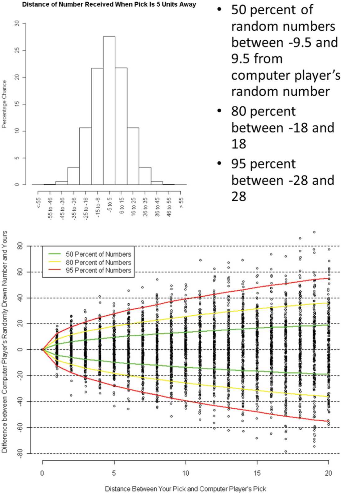
Examples of information provided to subjects to explain the stochastic process to them in the case where the variance was equal to 40.
While seemingly complicated, the math behind the Brownian motion formalization is quite simple and offers a number of attractive properties. Given one known policy–outcome pair, the expected value of the outcome that another policy produces is a linear extrapolation just like in the canonical model, but it is stochastic. The variance around the expected outcome at any point is the product of the Brownian variance and the size of the move from the known policy to the new one. Thus, the variance around this expected value increases the further a new policy is away from the known policy. This uncertainty representation nicely approximates many real-life situations. We often may not know exactly how policies produce outcomes, but we do have a sense of which direction to tweak an existing policy to achieve different goals. It also approximates many situations in which one can be relatively confident about small changes and relatively uncertain about the consequences of more radical alterations. Finally, one can easily model relatively complex or relatively simple choice environments by changing the random walk’s variance.
While not a behavioral model, the Brownian motion framework, and our interest in mimicking and modifying, has interesting overlaps with classic theories of bounded rationality and incrementalism (Lindblom, 1959; Simon, 1978). In some situations, the model predicts the same behavior that a satisficing theory would. Under some conditions, optimizing in the Brownian motion model means mimicking policies which one knows are imperfect.
The Brownian uncertainty model has a number of applications. The substantive context of the predictions we test, and the abstract situation we created in the laboratory, is learning from others’ policies. Thus, our experiment speaks in part to the large and growing diffusion literature. (See Karch (2007) and Dobbin et al. (2007) for reviews.) Our focus on micro-mechanisms is unusual in the literature since little work has distinguished mechanisms from each other (Dobbin et al., 2007; Glick and Friedland, 2014) or addressed the challenge of distinguishing diffusion from independent choices (Volden et al., 2008). Thus, an experimental test of a deductive formal model marks a methodological divergence (exceptions include Baybeck et al., 2011; Tyran and Sausgruber, 2005; Volden et al., 2008). The model of mimicking and modifying and the experiment we use to test it, connect formerly disparate ideas in the literature. Our two key variables are similarity (Dolowitz and Marsh, 1996; Grossback et al., 2004; Volden, 2006; Volden et al., 2008; Volden and Makse, 2011) and complexity (Gormley, 1986; Mooney and Lee, 1999; Nicholson-Crotty, 2009; Volden and Makse, 2011). Previous work demonstrated, for example, a link between ideological similarity and policy diffusion (Grossback et al., 2004). We focus on the complexity of policy areas which is at least subtly different than at least some in the literature who focus on the complexity of particular policy instruments (Rice and Rogers, 1980; Volden and Makse, 2011). The difference is that in our approach, complexity is a trait of the challenge the actor is facing. Finally, our focus on modifying builds on ideas of policy ‘reinvention’ (e.g. Glick and Hays, 1991) including those which consider links between complexity and reinvention (Mooney and Lee, 1999; Rice and Rogers, 1980).
While the predictions and the lab setup are closely related to the diffusion literature, our experiment and results concern human behavior and decision-making capacity more generally. As early as Downs (1957) and Berelson et al. (1954), scholars of political behavior have argued that while most voters are uninformed, they follow informed members of their social groups to make political decisions. Lupia and McCubbins (1998) repeat this claim and argue that it can be rational for voters to do so; some experimental studies explore whether subjects do this in a rational matter (Ahn et al., 2013; Lupia and McCubbins, 1998; Ryan, 2011). However, the cue-taking literature generally focuses on binary decisions and invertible signals. The model on which we base our test offers a richer conception of the types of decisions and information involved in attempts to learn from others.
Propositions derived from Brownian motion
Callander (2008, 2011a,b) has used the uncertainty representation in models of delegation and of actors experimenting with new policies. Glick (2012) has incorporated the technology into an extensive learning and policy diffusion model that applies to situations in which one actor can learn from another. We focus on two testable predictions concerning ‘mimicking’ (adopting an existing policy) and ‘modifying’ (changing an existing policy for a different context). These predictions are explicit in, and central to, Glick’s model and implicit in Callander’s.
The two propositions we test are formally derived (along with a number of others) in Glick (2012). Rather than reproduce the derivations, we refer to the proposition numbers (1.1 and 3.3, see below) in Glick’s full model that correspond to the two predictions that we test experimentally so that interested readers can see them formally. Nevertheless, we very briefly introduce the basic model and notation in hopes of making the rest of the paper clear. The basic model has two players 1 and 2 with ideal outcomes
The model investigates player 2’s options after observing player 1’s policy and the outcome it renders while knowing the goal similarity and Brownian motion parameters. The
The
These predictions contrast with those that one would derive from traditional models (see above) where the policy mapping function is a constant linear shock. With that alternative uncertainty model, the optimal behavior is to always modify the policy by adjusting for the difference between the two ideal points. This makes the optimal new policy a simple linear extrapolation from the known point to the new ideal point. Note that the difference between the two is not just that players always modify with a simple linear shock. The degree of modification is always greater with the simple linear shock.
These propositions describe optimal behavior when learning from others under Brownian motion uncertainty. These predictions from the model are clear but somewhat counter-intuitive. They are thus ripe for experimental testing. Knowing when to mimic, when to modify, and how much to modify by is a tricky task comprising two major challenges: The challenge posed by the level of (dis)similarity between one’s ideal outcome and the outcome produced by the known policy–outcome pair, and the challenge posed by the level of policy complexity. Decreased similarity produces a larger gap between the policy that will in expectation produce the actor’s goal and the optimal policy. Increased complexity increases the degree to which an actor should discount information about the distance between the known policy’s outcome and the actor’s own ideal outcome. These two factors mean that learning from others in such an environment is potentially more cognitively demanding than learning from others if uncertainty is described by the canonical model. We call it cognitively demanding because it requires actors to incorporate additional information and to make potentially counter-intuitive choices even though under some conditions the optimal action is to mimic which may be a very easy choice to make and implement. The key source of additional complexity for decision makers is the fact that optimizing in the Brownian model requires incorporating mean and variance into distance versus uncertainty tradeoffs whereas the canonical model only requires distance calculations. The optimal action is not always an intuitive distance adjustment. Even when actors should modify a known policy, they should do so less than the distance between the known policy’s outcome and their ideal outcome would suggest. Given the counter-intuitive nature of these theoretical findings, it is far from clear that actors will learn to throw seemingly useful information away or discount it optimally degree.
3. Experimental design
To test the ability of experimental subjects to optimally mimic and modify, we presented them with a simple decision task. In each round they had to pick a number which represented an abstract policy or other input. Subjects were informed that a randomly drawn number, representing a stochastic policy shock, would be added to the number they chose to produce their final outcome. The subject’s goal was to end up with a final outcome, representing a policy outcome or other output, that was as close to zero as possible.
Subjects could learn something about the randomly drawn number by observing the action of another player who also chose a policy and had a stochastic shock added to it to produce a final outcome. Specifically, in each round we showed the subject a computer player’s choice, the random number that was added to it, and the computer player’s final outcome. The difference between the stochastic shock added to the computer player’s choice and the stochastic shock added to the human player’s choice was the product of a Brownian motion process whose variance depended on the experimental condition and the distance between the numbers picked by the two players. Essentially, subjects faced a decision problem where their ideal outcome was zero, but the further their chosen policy was from the computer player’s policy, the less information the computer player’s stochastic shock provided about their own stochastic shock (and thus their final outcome).
After seeing the computer player’s decision, subjects were asked to choose a number. A random shock was then drawn and added to the subject’s choice, and then their final outcome (number) was displayed. A new round then began and each subject was presented with another computer player’s number, shock, and final number. Each subject played for 100 rounds.
Subjects were instructed that if they chose the same number that the computer player chose (‘mimicking’), they would receive the same stochastic shock, and thus the same outcome as the computer player. This means we are assuming that the two decision contexts are identical such that the mimicked policy produces the same outcome for the second actor as it did for the first. 2 They were told that if they chose a different number, it would be subject to a different shock, which was defined by the Brownian motion process. We did not attempt to explain the concept of Brownian motion to subjects. Instead, we explained the stochastic component by explaining that the variability of the random number would grow the further away their pick was from the computer players’ pick. 3 To illustrate how the variance of the shock depended on the distance between their pick and the computer player’s pick, we showed them two sets of pictures, examples of which are in Figure 1. First, we showed them four histograms approximating the normal distributions from which their random shock was to be drawn. These four histograms corresponded to picking a number four different distances away from the computer player’s choice. The variance of the normal distributions increases as the distance between the subject’s pick and the computer player’s pick grew. We also showed them a scatter plot with two thousand points drawn from the distribution of shocks that would be drawn in their session. The distance from the computer player was on the x-axis and the shock was on the y-axis. Subjects were given handouts with these figures, and could consult them during the experiment.
Since the experimental task was relatively complicated, we included an additional check on subjects’ understanding of the process that turned the number they picked into their final outcome. After the experiment was completed, each subject responded to the prompt ‘Please write how you understand that the random number was drawn’. Two independent coders who were unfamiliar with the study’s goals coded these responses on a 1–4 scale, where a higher number indicated greater understanding. A majority of subjects’ responses were coded 4, and 85% of subjects’ responses were coded 3 or 4 by both coders. Removing subjects who scored lower than 3 does not substantively change the results reported in the next section. These open-ended responses give us confidence that the findings we report are not the result of subjects who did not understand the experimental task. Details of the coding procedure and examples of response that received each code are available in Appendix E.
Experimental predictions
In Glick’s (2012) article discussed above, two factors influence a player’s decision to mimic or modify: the complexity of the decision task and the degree of similarity between the player’s goals and the goals of the informed player. These are represented mathematically as the variance (simply σ2 after assuming a drift of 1) and the distance between the player’s goal and the known policy outcome (denoted Δ12). To test learning with Brownian motion uncertainty, we varied these two factors as experimental treatments in a 2 × 2 design. The subject’s goal (optimal policy outcome) was fixed at zero. The distance between the subject’s goal and the known policy’s outcome was either small (Δ12 = 10) or large (Δ12 = 20). The variance of Brownian motion process was also manipulated to make the task either complex (σ2 = 40) or simple (σ2 = 20). This operationalization of complexity fits our concept of ‘policy area’ complexity because it affects how well actors can predict the consequences of their policy choices. Table 1 shows these four experimental conditions. To ensure that subjects did not face seemingly identical tasks each time, the distance between the subject and the computer player was drawn from a uniform distribution on (E(Δ12) − 5, E(Δ12) + 5). 4 In all cases, the underlying trend or drift (μ) of the Brownian motion was 1.
Optimal actions.

The parameters were chosen to test the model’s predictions that players should mimic when tasks are more complex or when similarity is high, and modify when tasks are less complex or when similarity is low. The optimal policy choices for the experimental treatments are summarized in Table 1. We cross these two manipulations to produce four experimental conditions. We denote each condition using an uppercase ‘H’ or ‘L’ for the level of complexity and a lower case ‘h’ or ‘l’ for the level of similarity. Thus the ‘high-complexity–high-similarity’ condition is denoted by ‘H-h’, the ‘high-complexity–low-similarity’ condition is denoted by ‘H-l’, and so on.
In the H-h condition (1), subjects should always mimic; the high degree of similarity means that the computer player’s outcome is close to the subject’s ideal outcome while the high degree of complexity means that modifying introduces a great deal of risk. In the L-l condition (4), players should always modify because the computer player’s outcome is far from the subject’s ideal outcome and the low level of complexity reduces the risk introduced by modifying. In the L-h condition (3) and H-l condition (2) the expected value of Δ12 is on the cut point between modifying and mimicking. Depending on whether the draw of Δ12 is above or below E(Δ12) in a given round, players should either mimic or modify. Thus, optimal behavior would lead them to mimic half of the time and modify half of the time. When modifying, the optimal average modification would be five units. Also of interest is how subjects would behave if they ignored the complexity of the decision, that is, the aspect that makes the Brownian motion representation unique, and acted as though uncertainty was described in the same way as the canonical model. The canonical constant shock model would predict the same strategy (modifying by Δ12) in all four conditions. This strategy represents the prediction that subjects will simply subtract the difference between their goal and the other player’s outcome from the other player’s optimal action to achieve their goal of zero.
Comparing actual behavior with the optimal behavior as described in Table 1, as well as comparing this to how subjects would act under the canonical model, will show whether subjects are able to adjust their behavior to the kind of uncertainty described by the Brownian motion process. Comparing how close subjects come to optimal behavior across experimental conditions will show how subjects respond to different kinds of difficulty in learning from others. Specifically, we can determine how the complexity of a task affects optimal decision-making by comparing the H-h condition with the L-h condition and the H-l condition with the L-l condition. We can determine how the similarity (or lack thereof) between decision makers affects optimal decision-making by comparing the H-h condition with the H-l condition and the L-h condition with the L-l condition. Finally, comparisons between subjects in the L-h condition and the H-l condition will allow us to tell whether subjects respond in different ways to these two types of task difficulty.
We completed six sessions of the experiment with 86 subjects, who were undergraduates at a private northeastern US research university. Each session was randomly assigned to be a ‘high-complexity’ session or a ‘low-complexity’ session, and subjects within each session were randomly assigned to either high-similarity or low-similarity. Five subjects’ data were dropped for failing to comply with experimental instructions leaving 81 subjects in four experimental conditions. A total of 24 were in the H-h condition, 17 in the L-h condition, 20 in the H-l condition and 24 in the L-l condition. Subjects played the game for 100 rounds. We selected one round at random for payment. Subjects were paid US$10 minus the squared distance (in cents) between their outcome in the randomly selected round and 0. 5 They also received a US$5 show-up fee, and could earn up to US$12 from a risk preferences elicitation. 6 Average earnings were US$16.81 including average earnings of US$5.23 from the risk preference elicitation. The experiment was programmed and conducted with the software z-Tree (Fischbacher, 2007); sessions lasted approximately 1 hour.
Results
We first establish that subjects did not behave as they would under the canonical model. Figure 2 shows the percentage of decisions that, in expectation, would produce the subject’s ideal outcome; that is, decisions that would be optimal if uncertainty was characterized as in the canonical model, rather than via Brownian motion. In all four conditions, this percentage is around 10% in the first 10 rounds, but drops rapidly to less than 5% in all four conditions. Most subjects appear capable of understanding that optimal behavior with Brownian motion uncertainty is different from the more intuitive canonical model.
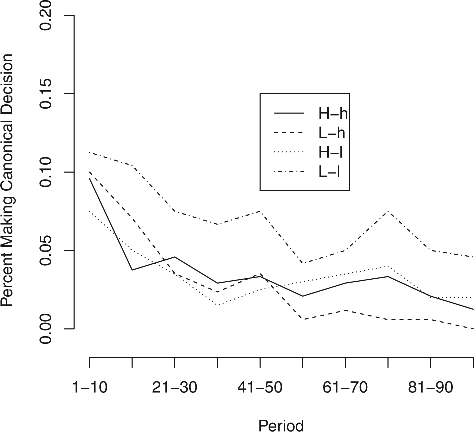
Percentage of decisions matching canonical model by 10-period blocks.
The fact that subjects did not behave as though they were facing canonical uncertainty does not, of course, mean that their actions conform to the predictions of the Brownian motion model. We use two metrics to measure how subject behavior compares with the theoretical predictions. The first is deviation from the optimal action: the number of units and direction that the subject’s action falls from the optional action as defined in Table 1. This number can be positive or negative. A positive deviation indicates over-modifying the action whose outcome was known, while a negative deviation indicates that the subject was too cautious and under-adjusted from the known action. One way to think of this measure is as a measure of bias in the statistical sense of the term where an unbiased subject would take, on average, the optimal action. Similarly, subjects in an experimental condition that produces unbiased results select the correct action on average, even if some generally over-adjust and some under-adjust. To give a sense of how subjects behaved over time, Figure 3 shows the average deviation from the optimal modification for each condition grouped into 10-period blocks. To conduct statistical tests, we analyze subject-level data by computing each subject’s average deviation from the optimal action across the final 20 rounds of play. 7 We then compare the distributions of these variables to the model’s predictions and across experimental conditions. Figure 6 shows these results graphically; Table 2 reports a full range of statistical tests.
Mean values by condition, with 95% confidence intervals.

Note:
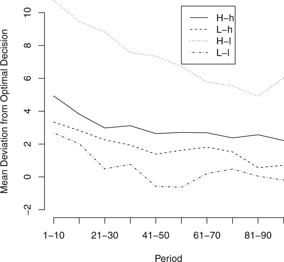
Mean deviation from optimal action by 10-period block.
The second metric is how frequently the subject mimicked the actions of the computer player. According to Table 1, subjects should always mimic in the H-h condition, should mimic when the computer player’s outcome is less than 10 in the L-h condition, should mimic when the computer player’s outcome is less than 20 in the H-l condition, and should never mimic in the L-l condition. This means that we should expect subjects to mimic 50% of the time in the L-h condition and in the H-l condition, every time in the H-h condition and never in the L-l condition. Translated into comparative static predictions, subjects should mimic the most in the H-h condition, mimic less frequently in the L-h and the H-l conditions, and mimic the least in the L-l condition. Figure 4 shows the over time trends in the percentage of mimicking decisions in each condition. We evaluate whether each decision to mimic or not was correct; that is, whether the subject mimicked if the optimal action was to mimic and modified if the optimal action was to modify. Figure 5 shows the percentage of correct decisions over time. For hypothesis testing we compute each subject’s percentage of times mimicking as well as the percentage of times each subject made the correct mimic/do-not-mimic decision in the final 20 rounds of play. Figures 7 and 8 show the results of this test graphically. In general, average subject behavior deviates from optimal behavior in two ways: a tendency to over-modify in high-complexity situations, and a bias towards modifying even when mimicking is the optimal choice.
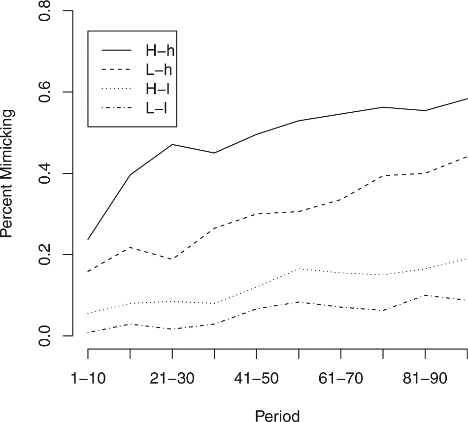
Percentage of decisions mimicking by 10-period block.
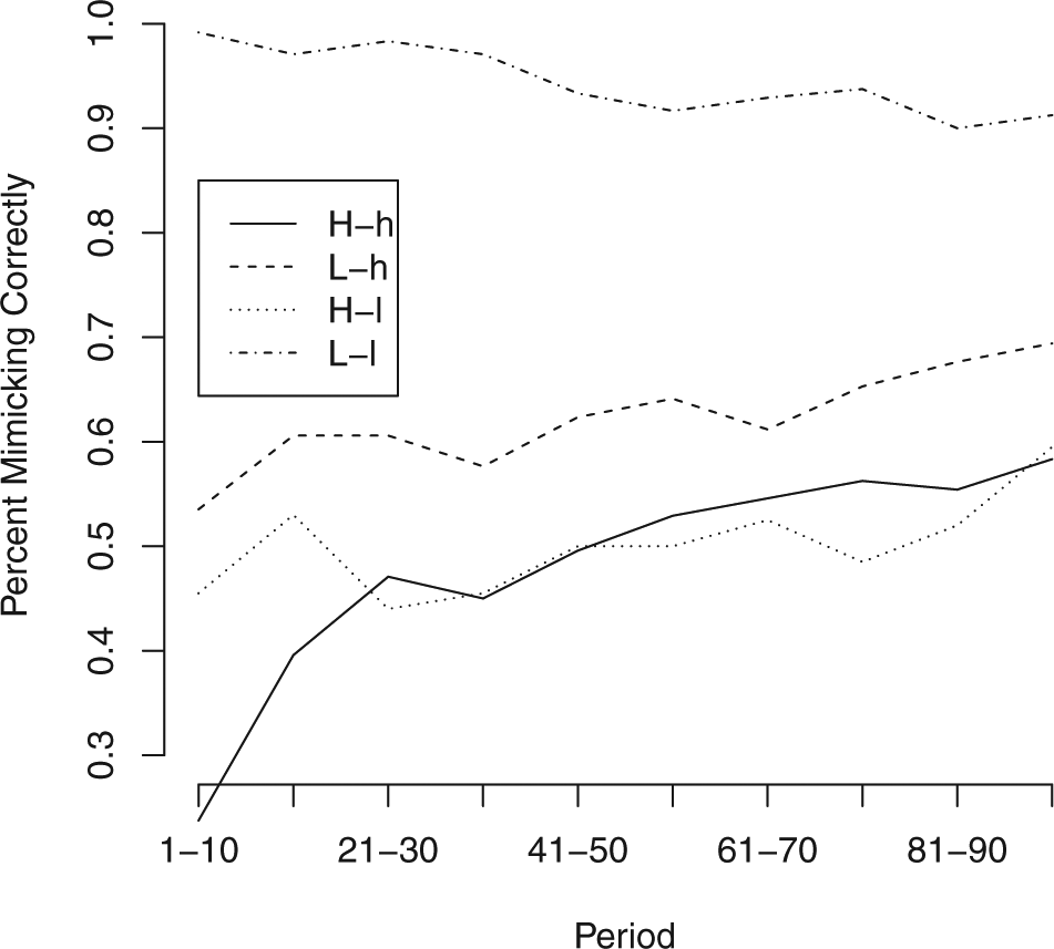
Percentage of decisions correctly mimicking by 10-period block.
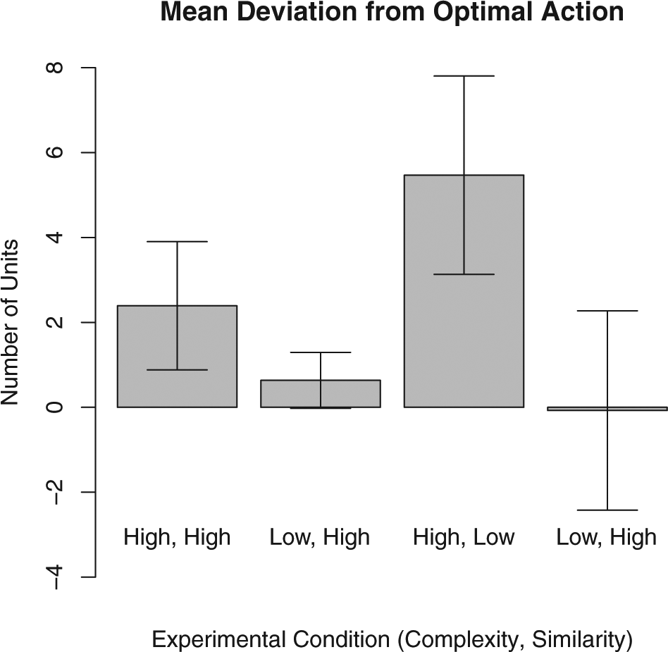
Subjects’ mean deviation from optimal action, last 20 rounds.
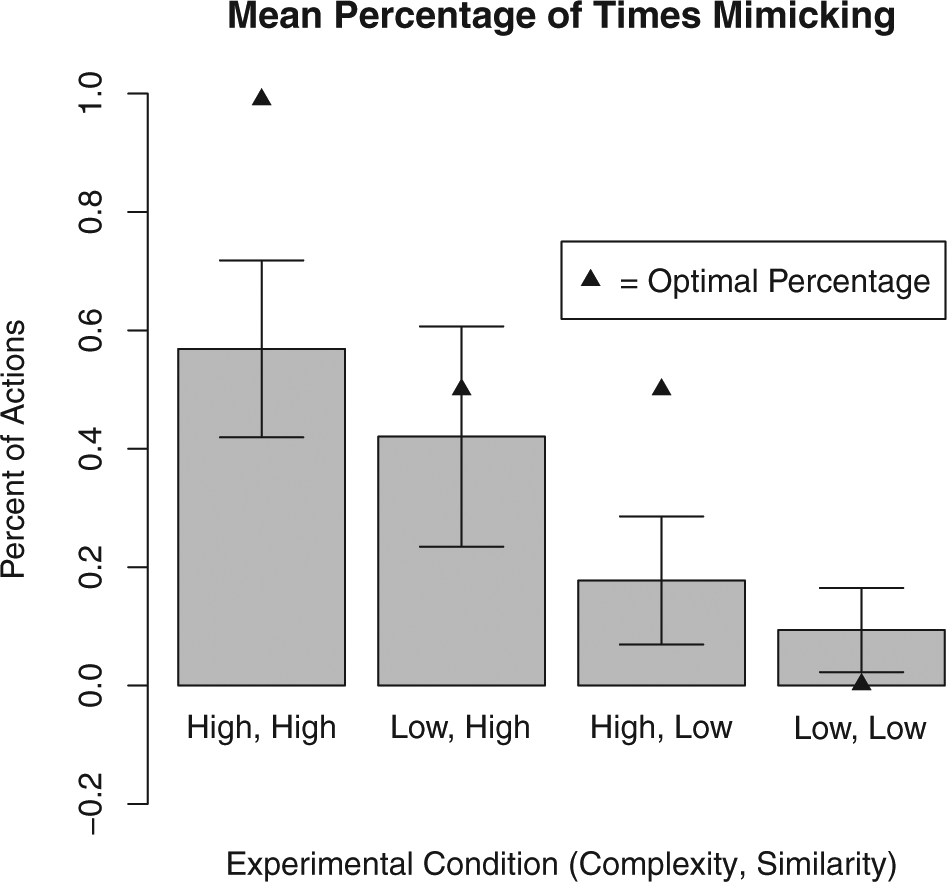
Subjects’ percentage of decisions that mimic, last 20 rounds with 95% confidence intervals.
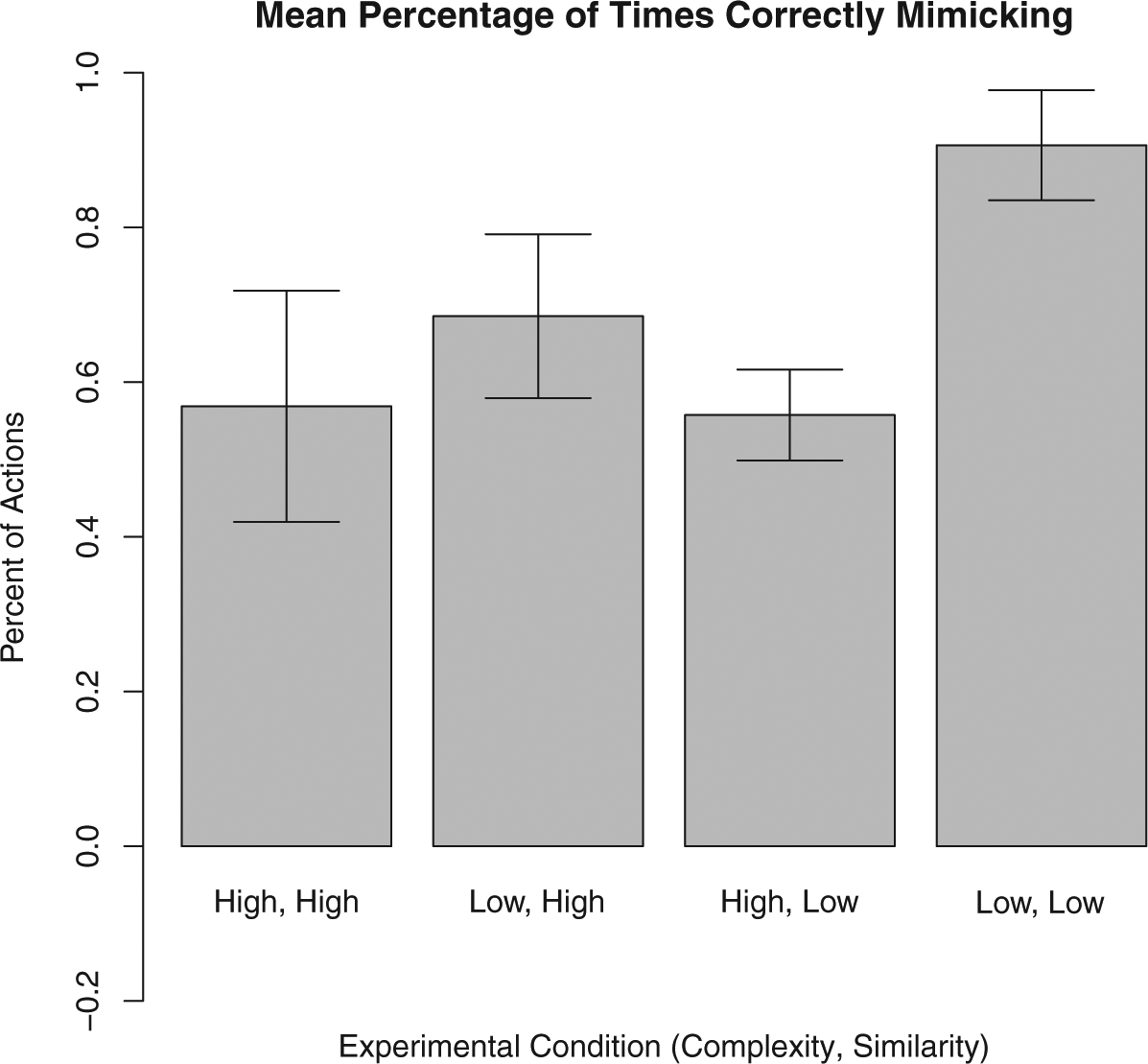
Subjects’ percentage of percentage of correct mimicking decisions, last 20 rounds with 95% confidence intervals.
We start by examining the L-l condition. This condition offers the cleanest test of subjects’ ability to behave in ways consistent with the Brownian motion model as the optimal action is always to modify, but by less than one would under the canonical model. 8 Specifically, the optimal action is to modify the first player’s choice by 10, halfway between the known policy and the choice that would be ideal under the canonical model. It does not produce the subject’s ideal outcome in expectation, but it is the best she can do given the uncertainty introduced by the Brownian motion process. Looking at overtime trends in Figures 3 and 4, we see that while subjects begin by over-modifying, by the 50th round the mean deviation approaches zero. Subjects in this condition almost never mimic at any point in the experiment. While the percentage mimicking increases over time, it never goes above 9% of subject decisions.
Looking at subject-level data aggregated over the final 20 rounds, we see a similar pattern that is largely in line with the model’s predictions. The average subject’s mean deviation from the optimal action is very close to, and not statistically different from, zero (p = 0.951, two-sided t-test). 9 The average subject mimicked nine percent of the time over these rounds, a statistically significant difference from the predicted zero (p = 0.017), but one that still shows subjects modifying in all but a substantively small number of cases.
Moving to the L-h condition, we again see mean results that are generally in line with the Brownian Motion model. In this condition, the higher similarity means that subjects should mimic half of the time. In the over-time results, we see the percentage of times mimicking increases over the course of the experiment but never exceeds 44%. Similarly, the mean deviation from optimal action in this condition decreases over time and approaches, though does not quite reach, zero. In the final 20 rounds, the average subject’s mean deviation was 0.63 units, a deviation that is marginally statistically different from zero (p = 0.078 two-sided t-test). The average subject mimicked 42% of the time in this period, a percentage that is not statistically different from the expected rate of 50% (p = 0.415, two-sided t-test); subjects made the correct mimicking decision in 69% of cases, a rate of correct decisions notably smaller than in the L-l condition, but higher than in either of the high-complexity conditions. Increasing the similarity between the subject’s goal and the known policy makes the decision task slightly more difficult, but does not appear to seriously degrade subjects’ performance.
In contrast, average behavior in the H-l condition shows that increasing the complexity of the decision causes subjects to deviate significantly from optimal behavior. Like in the L-h condition, subjects should mimic 50% of the time in this condition. Here, it is the higher degree of complexity that makes mimicking optimal half the time rather than the higher degree of similarity (see above). Figure 3 shows that decision-making in this condition improved little after the 40th round, with the average decision modifying by three units more than optimal. Similarly, Figure 4 shows that the rate of mimicking in the H-l condition is never above 19%, and that it stops increasing around round 60. Turning to subject-level behavior in the last 20 rounds, we find that the average subject deviated by 5.47 units, significantly different from optimal action (p < 0.000). This deviation is also significantly greater than the deviation in the L-l condition (p = 0.002) and in the L-h condition (p = 0.001). The average subject mimicked 17.7% of the time over this period, significantly less often than the optimal level of 50% (p < 0.000) and less often that subjects in the L-h condition (p = 0.036), but not significantly different from the 9% rate in the L-l condition. The average subject made the correct mimic/do not mimic decision 56% of the time, significantly less than the 69% figure for the L-h condition (p = 0.049). This low rate of correct decisions was not the result of mimicking too frequently, as 91% of these mistakes were from subjects not mimicking when mimicking was optimal. When faced with increased complexity, subjects mimic less and deviate more from the optimal action than in analogous low-complexity conditions.
Results from the H-h condition also suggest that subjects struggled with highly complex Brownian motion processes. In this condition, subjects should always mimic. Figure 4 shows that subjects mimicked in a higher percentage of decisions in this condition than any other, and that the percentage of decisions in which they mimicked increased over time. However, even in the final 10 rounds only 58% of decisions were mimicking, and the average decision was a modification of 2.2 units. The average subject mimicked 56% of the time in their final 20 decisions, significantly different from optimal rate of 100% (p < 0.000). The average subject’s mean modification in this period was 2.4, also significantly different from zero (p = 0.005). As in the H-l conditions, subjects faced with high-complexity Brownian Motion processes deviate significantly from optimal action even after 100 rounds of play and mimic significantly less than is optimal.
Finally, in addition to results based on average behavior, we examine heterogeneity of behavior across subjects. Figures 9 and 10 present histograms showing each subject’s average deviation during the final 20 rounds, percentage of times mimicking in the final 20 rounds, and percentage of times mimicking correctly in the final 20 rounds. We remove a few extreme values for graphical clarity. As these figures show, there was a great deal of heterogeneity in subjects’ actions even in experimental conditions where mean behavior was relatively close to theoretical predictions.
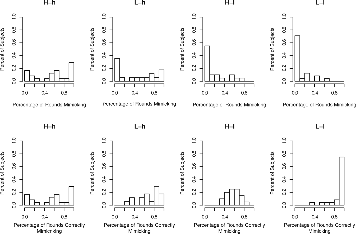
Histogram of subjects’ mimicking behavior, last 20 rounds with 95% confidence intervals.
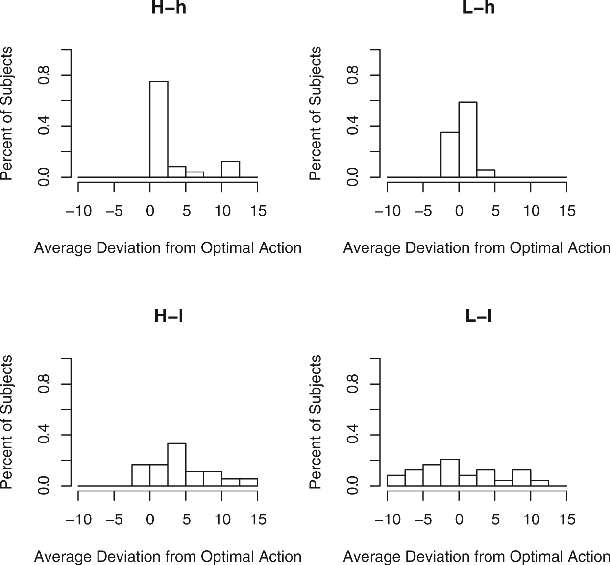
Histogram of subjects’ mean deviation from optimal action, last 20 rounds with 95% confidence intervals.
We highlight two aspects of heterogeneity across subjects. First, subjects in low-similarity conditions showed considerably more heterogeneity in their average deviation from optimal behavior than did subjects in high-similarity conditions. The average deviations by subjects in high-similarity conditions were tightly clustered. In the L-h condition 8 of 17 subjects averaged within 1.5 units of the correct action, and 15 of 17 subjects in this condition averaged within 2 units In contrast, most subjects in the low-similarity conditions either consistently over-modified or consistently under-modified. Thus, in the L-l condition, 6 of 24 subjects (20%) over-modified by an average of five units or more, while another 6 subjects under-modified by an average of 5 units or more. The H-h condition showed a similarly degree of heterogeneity though in this case the distribution was not symmetric around zero, and 8 of 20 (40%) subjects over-modified by at least 5 units.
Second, subjects in most conditions displayed a great deal of heterogeneity in their tendency to mimic. In particular, the bias towards action that we found looking at average rates of mimicking seems to affect some subjects more than others. Half of all subjects in the H-l condition and 35% of subjects in the L-h condition never mimicked, despite the fact that mimicking was called for in an average of half of all cases. Even in the H-h condition, where mimicking was always the optimal choice, 13% of subjects never mimicked. In general, Figure 9 shows that subjects in the high-similarity conditions adopted a much greater variety of mimicking strategies than subjects in the low-similarity conditions. However, this mostly reflects more subjects in the low-similarity conditions adopting a ‘never mimic’ strategy, a strategy that produced a very high rate of correct mimicking decisions in the L-l condition but fewer correct decisions in the H-l than in either of the high-similarity conditions.
The one condition without a great deal of heterogeneity in mimicking behavior was the L-l condition, a fact that provides further evidence of a bias towards action. In this condition, mimicking is never optimal, so a bias towards action will push subjects towards acting more correctly. Thus, subjects who are biased towards action and those who are not biased towards or against action will make the correct decision to modify. Indeed, in this condition 17 out of 24 (71%) of subjects never mimicked in the final 20 rounds, and only 12.5% mimicked in more than 25% of the final 20 rounds.
Discussion
This study presents subjects with a form of outcome uncertainty characterized by Brownian motion, a form that is more complicated than the outcome uncertainty in canonical models. While the canonical model presents subjects with a fairly simple decision task, Brownian motion presents them with two more complicated decisions: whether to modify a policy with a known but sub-optimal outcome and, if modifying, how much to modify by. Can subjects navigate these more complicated decisions? The broad answer is yes. Subjects do respond to this more complicated decision environment sensibly, although not quite optimally. Few subjects ignore the more complicated decision environment and act as though they are dealing with the canonical model. Further, their actions trend towards optimal behavior over time, and in the low-complexity conditions their behavior approximated, on average, optimal behavior.
Nevertheless, even after an extended period of learning, subjects do not learn from others in fully optimal ways. The results from this experiment suggest two things about learning from others in situations where policy uncertainty is described by a Brownian motion process. First, the degree to which subjects’ behavior is described by the Brownian motion model depends on the complexity of the decision they face. In situations where complexity was low, subject’s behavior was generally in line with optimal behavior. However, when complexity was higher, subjects deviated from the predictions of the model in important systematic ways. Subjects underestimated the effect that this complexity has on their decisions and over-modified the policy that they were learning from. This may not come as a big surprise. Complexity, which refers to the amount of variance in the Brownian process, is the element that separates uncertainty as described by Brownian motion from uncertainty as described in the canonical model. The more complex a problem is, i.e. the more uncertainty there is between policies and outcomes, the larger the gap in optimal action in the two models. Unfortunately, this suggests that situations where a Brownian motion conception of complexity offers the greatest theoretical advance over the canonical model are also those where the Brownian motion model does the worst job of predicting behavior.
Second, particularly when complexity was high, subjects showed a bias towards action. In high-complexity conditions subjects make fewer correct mimicking decisions because they do not mimic in cases where mimicking is optimal. In the low-complexity condition where the optimal rate of mimicking was non-zero subjects still made correct mimicking decisions only two-thirds of the time and mimicked less often than optimal, although not by a statistically significant margin. This may be evidence of action bias (Kahneman and Tversky, 1984; Patt and Zeckhauser, 2000), in which a norm of action causes decision makers to take an action even when inaction is optimal. In the Brownian motion context, decision makers should sometimes mimic a known policy (inaction) despite knowing that it does not produce their ideal outcome. We suggest that subjects in this experiment are operating under a norm of adjusting their behavior in response to seemingly useful information, and against simply discarding this information. The sense that they will regret violating this norm in the case of a bad outcome creates a bias towards action. This suggests that the predictions of Brownian motion models may fare particularly poorly in situations where inaction is a major prediction. When it is optimal to discard information the temptation to tinker may be too great to resist. Alternately, the bias towards action may be highly dependent on the prevailing norms of the decision environment. In some decision scenarios, a norm of inaction or copying 10 might help subjects to act more rationally.
Conclusion
Brownian motion offers a more nuanced, flexible, and theoretically attractive representation of uncertainty. It has applications to institutions and individuals in a wide variety of political settings, of which our test of learning from others is only one. However, behaving consistently with equilibrium predictions predicated on this underlying uncertainty model is more difficult than behaving consistently with the canonical model of uncertainty. Despite this difficulty, our experiment finds that individuals did a respectable job of learning from others’ choices in a rich and challenging choice environment.
At the same time, we find that subjects’ choices deviate from full rationality in systematic ways. Most notably, people are better at working with variations in goals than they are with highly uncertainty policy outcomes. These results do not suggest rejecting the use of Brownian motion to model uncertainty in decision-making. Instead, they suggest caution in interpreting the predictions of these models in certain situations. The biases our results demonstrate represent systematic deviations from the behavior predicted by Brownian motion models in situations where the Brownian motion process is highly complex. Taking these biases into account when interpreting the predictions of these models will help empirical and formal scholars use them with proper care.
Our findings offer twists on two cognitive biases that affect decision-making: action bias (as discussed above) and anchoring bias. Anchoring describes the tendency of decision makers to choose actions that are closer to a numerical ‘anchor’ than they would if the anchor, however random, was not present (Tversky and Kahneman, 1974; Wilson et al., 1996). In most anchoring experiments, subjects are asked a question requiring a numerical answer after being presented with a numerical value that is unrelated to the question. These studies find that subjects’ answers are influenced by the value of the ‘anchoring’ number. In the present study, the computer player’s decision, which is presented immediately before the subject makes a decision, provides a potential anchor. Anchoring is usually thought of as a bias that leads actors to act irrationally by giving weight to an irrelevant anchor. However, since rational behavior in the context of Brownian motion uncertainty demands making a smaller modification to a known policy than might seem intuitive at first glance, anchoring bias may actually help actors behave optimally. Indeed, the original mimicking and modifying model may be characterized as a theory where a meaningful rather than random anchor makes anchoring rational.
Instead, we find that subjects deviate too far from this informative anchor. Given that people anchor when the initial values are completely arbitrary, the fact that they deviate too far from informative starting points is noteworthy and suggests interesting overlaps between behavioral economics and rational choice work using sophisticated uncertainty models. Alternately, subjects may be anchoring on something other than the computer player’s decision, for example, the distance between the computer player’s ideal outcome and their own. 11 In either case, while this study’s aim was not to test the effect of psychological biases these results suggest that the application of anchoring theory to action in the context of Brownian motion uncertainty is not straight-forward.
One important substantive application of our findings is the diffusion of policies among the states and in other contexts. One important diffusion question is how well policy makers can learn from existing policies and implement their lessons in different contexts; for example, how a state such as New Hampshire can learn from the policies of a state such as California. With only some extrapolation to policy diffusion, the lab results suggest that policy makers in New Hampshire likely do a good job adjusting for the fact that they may have very different policy needs than California. However, in complex policy areas these different needs may lead them to over-adjust a policy, while a bias towards action may lead them to change a policy even when simply copying the policy is the best course of action. This is potentially problematic since complex policy areas may be the areas in which smaller states most rely on learning from bigger and better resourced ones. Needless to say, attempting to verify our findings in applied policy settings with observational data would be ideal but challenging. Nevertheless, at a minimum, one could use interviews, surveys, and/or survey experiments with actual policy makers to test whether they perceive these challenges, and whether they have more confidence in adjusting for goal similarity than for complexity.
Our initial empirical investigation of learning and Brownian motion suggests several other lines of future work. One angle would be to test how performance varies with substantively important changes in the environment. One could, for example, run the same experiment on a pool of individuals with experience making policy choices, allow people to work in teams like they often do in policy choice settings, and/or add a level of realism by adding an accessible concrete story to the choices they are making. Moreover, recent theoretical work concerning learning in plausible real-world situations with more than one existing policy to learn from can easily provide additional hypotheses to test. One could use a very similar experiment to test how well individuals incorporate information from two known policies (Callander, 2011b; Glick, 2012), or how well they balance similarity and competence tradeoffs when choosing from multiple actors to learn from (Glick, 2012). As in this paper, testing these predictions would provide insight into decision tactics with real applications and into the validity of the underlying uncertainty innovations. In addition, our model uses a simple decision-theoretic environment where subjects do not interact. An important next step is to investigate behavior in game-theoretic environments where actors’ beliefs about how others will respond to Brownian motion uncertainty are important.
Footnotes
Acknowledgements
A previous version of this paper was presented at the 2010 MPSA Conference. We’d like to thank Nolan McCarty, Adam Meirowitz, Graeme Boushey, the Princeton Laboratory for Experimental Social Science, and participants at the Research in American and Comparative Politics Colloquium at Boston University. All errors are, of course, our own.
Declaration of Conflicting Interests
The author(s) declared no potential conflicts of interest with respect to the research, authorship, and/or publication of this article.
Funding
The author(s) disclosed receipt of the following financial support for the research, authorship, and/or publication of this article: This project received funding from the Princeton Laboratory for Experimental Social Science, Boston University, and the Robert Wood Johnson Foundation Scholars in Health Policy Program.