Target shape approximation of funicular surfaces by load control using RBF interpolation

Abstract

Existing methods for form-finding prioritize discovering optimal shapes under design load conditions, often overlooking the designer’s shape preferences. To address this problem, this research relaxes the load condition and develops a user-friendly form-finding tool that encapsulates a new method for obtaining funicular surfaces that pass through user-prescribed points through load control. The method involves generating smooth load distributions via RBF interpolation of nodal loads, which are repeatedly adjusted so that the equilibrium shape is close enough to the target points. For faster convergence, the step size of the load adjustment is automatically determined through a coarse line search, and a warm start is introduced in form-finding with the dynamic relaxation method. Despite uneven load distributions, the method ensures high accuracy in approximating the surface shape to the desired points while preserving funicularity against the load distributions. Additionally, the resulting load distribution gives designers valuable feedback on the specified target points, as the degree of load non-uniformity indicates the deviation from the equilibrium shape for uniformly distributed loads.

Keywords

Funicular form-finding RBF interpolation digital design tool particle spring system

Introduction

Funicular analysis

The equilibrium shape of a cable structure for a given support and load condition is called the funicular shape. Since cables cannot carry compression and bending forces, funicular cables experience only tensile forces. By inverting the shape or the load directions, an anti-funicular shape can be obtained in which all the internal forces are compression and include small bending. Hereinafter, funicular and anti-funicular are simply referred to as funicular without distinguishing between them.

The funicular shape against self-weight is particularly called catenary, and catenary curves and surfaces have been employed as a structural shape of masonry and shell structures through history¹ due to their favorable structural property against gravity. Parabolic curves and surfaces are other characteristic funicular shapes that are in equilibrium under uniformly distributed vertical loads. Since parabolic arches can span large distances, they have been widely employed in the shape design of bridge structures.²

Computer-aided design has made it possible to simulate funicular shapes, replacing the need for labor-intensive physical experiments. Block and Ochsendorf³ and Block⁴ presented Thrust Network Analysis (TNA) which integrates projective geometry, graphic statics, and linear optimization to identify funicular shapes under gravitational load. The TNA-based funicular design has been further extended to construct interactive design frameworks for compression-only shapes⁵ and combined compression-tension structures.⁶ Harding and Shepherd⁷ developed a form-finding method using zero-length springs with dynamic mass, which was later applied to designing a timber plate funicular shell.⁸ Bruggi⁹ augmented a force density method, originally developed for the form-finding of network structures,¹⁰ for the funicular analysis of arcuated structures. Michiels et al.¹¹ generated funicular polygons through graphic statics to ensure a compression load path that can withstand lateral earthquake loads.

Even earlier, Kilian and Ochsendorf¹² developed an interactive method to find equilibrium shapes of particle spring systems, which are physics-based models that simulate the behavior of particles connected by springs. Piker¹³ developed the Kangaroo plug-in for Rhinoceros^® and Grasshopper^® to obtain equilibrium shapes with a user-friendly interface. In particular, Kangaroo-based particle-spring systems have been used to obtain funicular shapes in many studies.^14–16

Integrating shape preference

Since the shape plays a critical role in the structural performance of shell structure, the above funicular form-finding processes are mostly based on mechanical properties. However, if the shape is to be modified based on other factors such as functionality, legal regulations, and the designer’s preference, the user must follow the repetitive procedure of changing the form-finding inputs and parameters based on the results obtained.

Design exploration with optimization algorithms is a widely used approach for integrating factors beyond structural performance. In this approach, the designer selects their preferred shape from the generated solutions. Pugnale and Sassone¹⁷ proposed a structural optimization method of NURBS surfaces using a genetic algorithm, where the designer, as a decision maker, controls the evolution process of solutions. Mueller and Ochsendorf¹⁸ also proposed an interactive evolutionary algorithm for structural optimization, which allows the selection of candidate designs during optimization. Other studies have suggested multi-objective optimization algorithms to generate a wide range of solutions, providing the designers with the freedom to choose their preferred design after optimization.^19,20

Nevertheless, these approaches become increasingly difficult to put into practice as the design space expands and the objectives become more complex. If the form-finding process can incorporate the designer’s rough idea of the desired shape based on architectural planning beforehand, such a method enables obtaining a shape that meets various requirements with less effort.

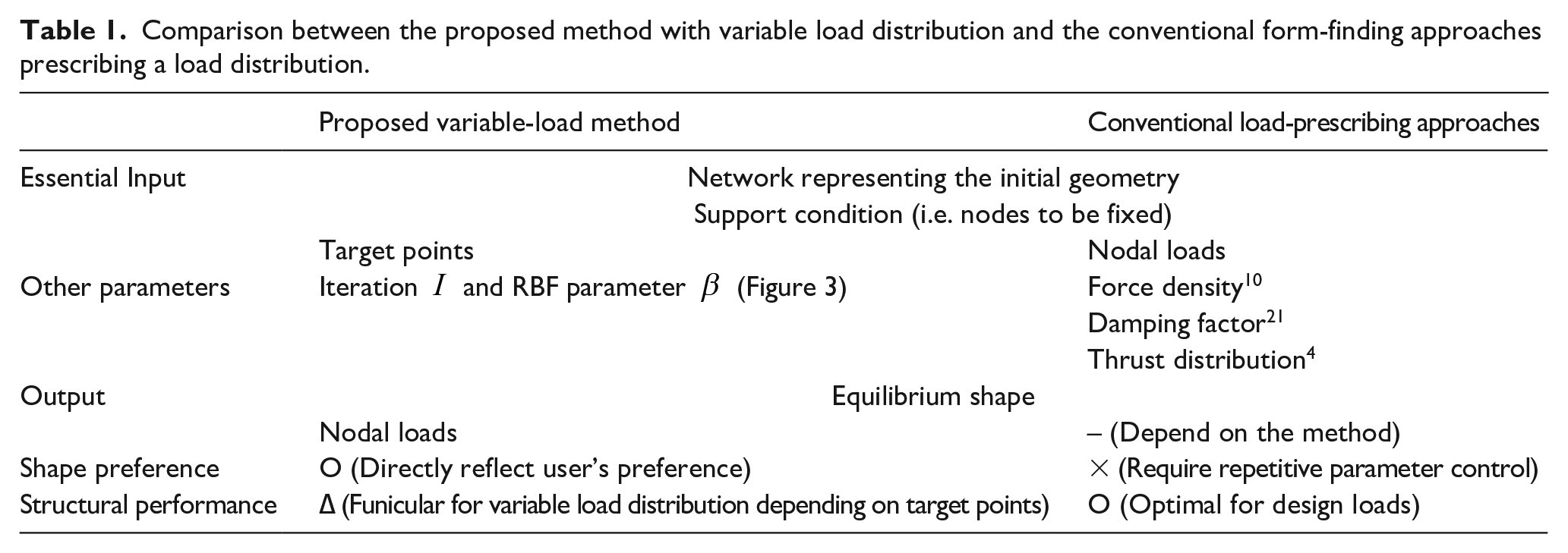
The problem here is how to reconcile funicularity and the designer’s intention. In general, the funicular analysis is performed under the assumption of self-weight or uniformly distributed loads, but this does not necessarily result in an accurate approximation of the target shape. The method developed in this paper, which is briefly compared with conventional form-finding approaches in Table 1, is based on the idea that relaxing the load condition can bring the funicular shape closer to the target shape. Such a funicular analysis method can prioritize the designer’s intention, which has been regarded as relatively unimportant, while still ensuring a certain degree of structural rationality.

Table 1.

Comparison between the proposed method with variable load distribution and the conventional form-finding approaches prescribing a load distribution.

	Proposed variable-load method	Conventional load-prescribing approaches
Essential Input	Network representing the initial geometry
	Support condition (i.e. nodes to be fixed)
	Target points	Nodal loads
Other parameters	Iteration $I$ and RBF parameter $β$ (Figure 3)	Force density¹⁰
		Damping factor²¹
		Thrust distribution⁴
Output	Equilibrium shape
Output	Nodal loads	– (Depend on the method)
Shape preference	O (Directly reflect user’s preference)	× (Require repetitive parameter control)
Structural performance	∆ (Funicular for variable load distribution depending on target points)	O (Optimal for design loads)

Mathematical surface representation

Shell structures usually have an organic shape, and mathematical surface representations such as Bézier, B-spline, NURBS, and T-spline are preferred to model shell shapes that are desirable for designers. These representations have an advantage in that they can create a smooth surface from discrete inputs such as control points and knot vectors; in other words, the designers do not have to specify every single point on the surface but only need to adjust some critical points and parameters that represent the surface.

Kimura and Ohmori²² formulated an optimization problem for shell structures to find an optimal shape, thickness, and topology of NURBS surfaces. Although this method can reflect the designer’s intention by specifying the initial shape for optimization, the optimal shape does not necessarily retain the shape features important to the designer because the control points are relocated by optimization.

Another difficulty in mathematical surface representations is that the users must specify the connectivity of the control points. To make matters worse, In Bézier, B-spline, NURBS, the connectivity of control points must form a regular grid, which might be a constraint when specifying the surface shape. While T-spline allows for customizable connectivity to the control net, users may find this task to be burdensome.

Surface interpolation

An alternative to the input for shape definition might be points that the surface passes through. This input setting is more user-friendly because there is no need to specify the connectivity of the input points. In this case, interpolation techniques enable obtaining surfaces passing through the points.

Polynomial interpolation is one of the simplest methods to construct a surface from a given set of points. To achieve an exact polynomial interpolation, the degree of the interpolant must be greater than or equal to the number of points being interpolated. The most common formula for this polynomial is the Lagrange polynomial constructed by a combination of the Lagrange bases. However, higher-degree polynomial interpolation may be susceptible to oscillations known as Runge’s phenomenon.

Unlike polynomial interpolation, spline interpolation divides the data into smaller segments and fits separate polynomials of lower degree to each segment. In particular, cubic spline interpolation is widely used because it ensures the C0, C1, and C2 continuity of the interpolant. However, applying multivariate spline interpolation to irregularly spaced data is generally challenging. One exception is the solvers by ALGLIB that fit bicubic splines to the scattered data.²³ Another drawback is that spline extrapolation may result in excessive values since the interpolant is determined based solely on the conditions for passing through the points and for the first and second derivatives at the points. For instance, natural cubic splines, which are the most common variant of cubic splines, assume that the function is linear beyond the boundary known points.²⁴

The Inverse-Distance Weighting (IDW) method²⁵ provides an exact interpolation of irregularly-spaced data points, and IDW-based methods are frequently used in the Geographical Information System (GIS).^26,27 However, general IDW methods never predict values beyond the maximum and minimum reference values, and may cause a so-called bull’s eye effect, concentric circles around the reference points in the contour map of the interpolation surface, which degrades the esthetic property of the interpolation result.^28,29

Kriging, a prevalent method in the area of geostatistics,³⁰ is another interpolation method based on the spatial covariance structure of the samples. The results of Kriging interpolation can also be utilized as a surrogate model that replaces simulations that require a high computational load.^31,32 Since the Kriging model also provides uncertainty information at the interpolated values, an optimization method has also been proposed to simultaneously improve the approximation accuracy of the response surface and search for the global optimal solution.³³ However, the construction of a Kriging model is generally time-consuming.^34,35

Radial basis function (RBF) interpolation uses a weighted sum of RBFs centered at each data point. This method, much like IDW and Kriging, is suitable for interpolating scattered data points. Additionally, with the selection of the RBF type and the adjustment of RBF parameters, the interpolant can be tuned with ease, which offers more flexibility in controlling the smoothness of the interpolant and the extrapolation behavior. Moreover, RBF interpolation is computationally efficient because it involves calculating the distances between data points and solving a straightforward linear system of equations, which can be efficiently handled using numerical and parallelization techniques.

Objective

While numerous form-finding methods exist, only a limited number of studies have delved into the integration of shape preferences beyond structural feasibility. In order to make form-finding more accessible for non-structural-engineering sectors, this paper offers a user-friendly tool, which was published on July 31st, 2023 on the Food4Rhino platform. This tool facilitates the generation of various funicular shapes passing through user-prescribed points by controlling a smooth load distribution generated by RBF interpolation. Notably, this method does not necessitate any prior information about the load condition, unlike conventional form-finding approaches.

The load modification process is fully automated to improve usability. In this process, a coarse line search and a warm start are introduced to improve the convergence property. This tool also aims at providing visual feedback on not only the funicular shape but also the associated load distribution to evaluate structural feasibility.

Structure of this paper

The remainder of this paper is organized as follows. The second section, “RBF interpolation,” explains the basics of RBF interpolation. The third section, “Target shape approximation by load control using RBF interpolation,” describes the details of the proposed method. The fourth section, “Tool development,” explains the tool encapsulating the proposed method. The fifth section, “Numerical examples,” provides numerical examples demonstrating the effectiveness of the proposed method. The sixth section, “Conclusion,” presents the conclusions of this study.

RBF interpolation

This section briefly introduces the basics of interpolation using a radial basis function (RBF). An RBF $ϕ (r) : ℝ \to ℝ$ is a function that outputs a real value depending on the distance input $r$ . The input to the RBF in this research is the distance between a certain point and a reference point given by the designer, and there is no difficulty in using the usual Euclidean distance as the metric.

Let $c$ denote a positive constant parameter. Among popular choices for the RBF $ϕ$ such as thin-plate spline $ϕ (r) = r^{2} \log r$ , inverse quadratic $ϕ (r) = 1 / (1 + c r^{2})$ , multi-quadric $ϕ (r) = \sqrt{1 + c r^{2}}$ , bi-harmonic $ϕ (r) = r$ , tri-harmonic $ϕ (r) = r^{3}$ , we chose the following Gaussian function as the RBF to be utilized hereafter.

ϕ (r) = \exp (- c r^{2})

(1)

RBF interpolation is a method to find an interpolant $f (x)$ given a set of input-output pairs ${x_{i}, y_{i}}$ $(i = 1, \dots, n)$ using an RBF, which is expressed as

f (x) = \sum_{i = 1}^{n} w_{i} ϕ (∥ x - x_{i} ∥)

(2)

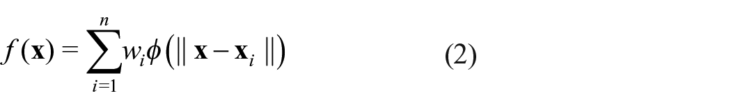
where the weight parameters $w_{i}$ $(i = 1, \dots, n)$ are determined by solving the following system of linear equations such that exact interpolation is ensured at the given input-output pairs:

Φ w = y

(3a)

w = [w_{1}, \dots, w_{n}]^{⊤}

(3b)

y = [y_{1}, \dots, y_{n}]^{⊤}

(3c)

Φ = [\begin{matrix} ϕ (∥ x_{1} - x_{1} ∥) & \dots & ϕ (∥ x_{1} - x_{n} ∥) \\ ⋱ & ⋮ \\ s y m m e t r i c & ϕ (∥ x_{n} - x_{n} ∥) \end{matrix}]

(3d)

Target shape approximation by load control using RBF interpolation

Limitation of RBF interpolation for direct approximation of shell shapes

The proposed method takes a mesh $M$ , nodes in the mesh to be supported, and target nodal positions $({\bar{x}}_{i}, {\bar{y}}_{i}, {\bar{z}}_{i})$ $(i = 1, \dots, n)$ as inputs to adjust the z-coordinates of the mesh nodes so that the transformed mesh $\tilde{M}$ passes through the target nodes.

With this input-output setting, one of the most straightforward approaches might be directly interpolating the support and target nodal positions using RBF interpolation. However, due to C1 continuity of the resulting interpolating surface, bending forces might be dominant around fixed positions, as illustrated in Figure 1.

Figure 1.

Structurally unfavorable shape interpolating the support and target positions. For simplicity, a curve rather than a surface is illustrated.

Load control using RBF interpolation

Instead of directly interpolating the point locations, consider interpolating the vertical load distributions applied to mesh nodes. That is, RBF interpolation is performed with $x_{i} = ({\bar{x}}_{i}, {\bar{y}}_{i})$ $(i = 1, \dots, n)$ such that $f (x_{i})$ equals to $p_{i}$ , the magnitude of the vertical load at target point $i$ . The interpolant $f (x)$ represents the vertical load distribution parametrized by ${p_{1}, \dots, p_{n}}$ that aims to deform the mesh into a shape passing through the target points.

Although it is difficult to explicitly obtain the load ${\bar{p}}_{i}$ that leads to the target shape, the value of ${\bar{p}}_{i}$ can be obtained approximately by repeating the following update formula until convergence:

p_{i}^{t + 1} \leftarrow p_{i}^{t} + α ({\bar{z}}_{i} - z_{i}^{t})

(4)

where $p_{i}^{t}$ and $z_{i}^{t}$ denote the values of $p_{i}$ and $z_{i}$ at iteration $t$ , respectively, and $α \in ℝ^{+}$ is a step size. Since there are $n$ target nodes and $n$ degrees of freedom for controlling the load distribution, $p_{i}$ $(i = 1, \dots, n)$ is uniquely determined.

Line search for determining the step size

In equation (4), the smaller the value of $α$ , the more steps are required to converge. On the other hand, assigning an excessive value to $α$ increases the risk of divergence. Therefore, the value of $α$ must be determined with careful adjustment.

Considering that the displacement monotonically increases as the step size increases, finding the optimal step size is a convex optimization problem. In order to efficiently determine an appropriate step size without spending too much time on finding the optimal one, this study adopts the following coarse line search method.

Let $α_{0}$ denote an initial step size and $γ > 1$ a constant multiplication factor. Hereafter, the step size is repeatedly multiplied/divided by $γ$ to increase/decrease its value. First, to decide whether to keep, increase, or decrease the step size, the equilibrium shapes are obtained for the three load cases with $α = α_{0}$ , $γ α_{0}$ , and $α_{0} / γ$ substituted into equation (4). Depending on the errors between the target height and the equilibrium shapes, the step size adjustment branches into either of the following three processes.

If the error is the smallest when $α = α_{0}$ , $α_{0}$ is regarded as near-optimal for $α$ .

If the error is the smallest when $α = γ α_{0}$ , the multiplication by $γ$ is iterated until the error begins to increase, and the value of $α$ that yields the smallest error is considered as approximate optimal.

If the error is the smallest when $α = α_{0} / γ$ , the division by $γ$ is iterated until the error starts to increase, and the value of $α$ that results in the smallest error is considered as approximate optimal.

The value of $α$ obtained by the above procedure is used as the initial value $α_{0}$ for the next line search. The value of $α_{0}$ for the first line search is $0.01$ , and the value of $γ$ is $10.0$ in this study.

Warm start for form-finding

In the proposed method, the load distribution is modified sequentially, and the dynamic relaxation (DR) method is executed to obtain the equilibrium shape after each modification. If the initial shape is similar to the equilibrium shape, the dynamic relaxation method requires fewer iterations for convergence. Therefore, the method involves a warm start, which is a technique where an algorithm is initialized with a solution obtained from a previous run.

Figure 2 illustrates the difference between cold and warm starts. Although the dynamic relaxation method reaches the same equilibrium shape regardless of the initial solution, the warm start requires fewer iterations to converge owing to inheriting the previous equilibrium state. Since the load distribution change diminishes in later steps, the advantage of adopting the warm start becomes more pronounced as the step repeats.

Figure 2.

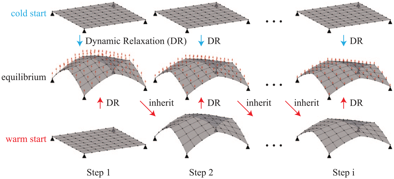
Difference between cold and warm starts in the proposed process.

Tool development

User interface

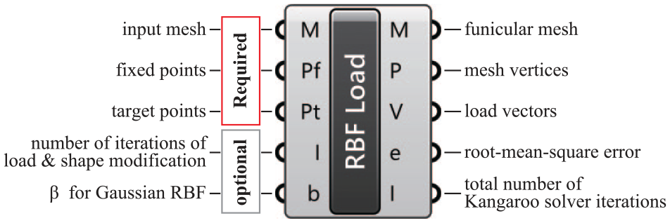
This section explains the developed Grasshopper© component that encapsulates the proposed method. Figure 3 illustrates the inputs and outputs. The necessary inputs include the mesh representing the connectivity of the network structure, the points constrained to move, and the target points. The rest of the inputs are optional, and the default values for the number of iterations and the $β$ value for the Gaussian RBF are $10$ and $1.0 \times 10^{- 5}$ , respectively. If the optional values have been specified by the users, the default values are replaced by the specified ones. The outputs include the deformed mesh, the mesh vertices, the nodal load vectors, the root-mean-square error (RMSE) of the target shape approximation, and the total number of analyses required to reach equilibrium states using the Kangaroo solver.

Figure 3.

RBF Load component that encapsulates the proposed method.

Workflow of the tool

The whole workflow of the proposed method is described in Figure 4. First, the nodal loads are initialized as 0 after processing the inputs. The height differences between the target nodes and the mesh are measured, and the load values associated with the target points are computed by equation (4). Then, the nodal loads applied to the mesh vertices are computed by RBF interpolation. This tool employs the Kangaroo solver with default optional parameters, for example, the stiffness of mesh edges, the rigidity of supports, and convergence criteria, to obtain an equilibrium shape for the nodal loads. This subroutine of load and shape modification is repeated until it reaches the specified number, and the tool finally processes the outputs.

Figure 4.

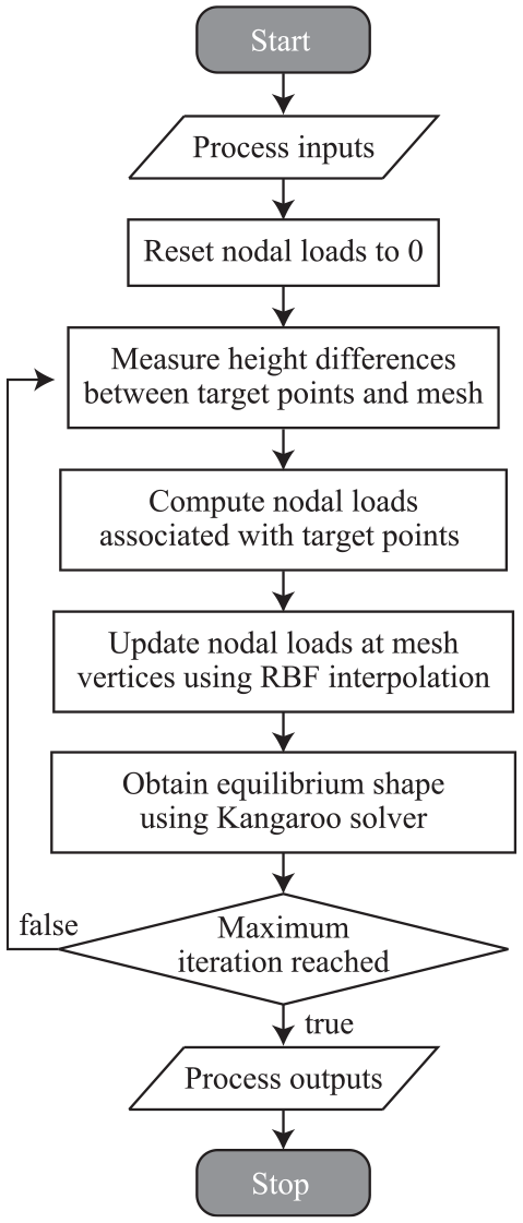
Workflow of the proposed method.

Numerical examples

20 × 10-grid mesh

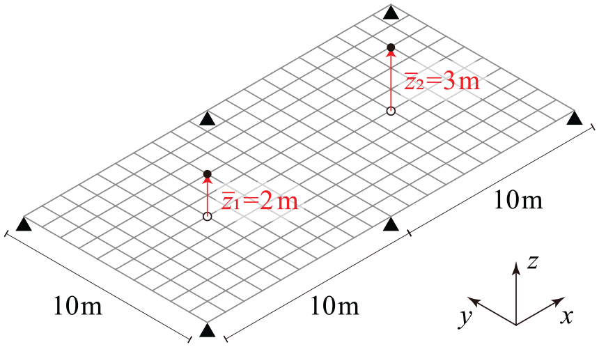
Through a relatively simple mesh, as shown in Figure 5, we verify the validity of the proposed method and investigate the effect of hyperparameters on the results in this section. The mesh has a $20 m \times 10 m$ plan, and $21 \times 11 = 231$ nodes are regularly spaced at the interval of 1 m. A total of 430 edges connect the neighbor nodes. The four corners and the mid-points of the long side are pin-supported. Two target nodes are placed in the middle of the short side and at the quarter of the long side. The heights are ${\bar{z}}_{1} = 2.0 [m]$ and ${\bar{z}}_{2} = 3.0 [m]$ , and the RBF parameter $β$ is ${1.010}^{- 5}$ if not specified. The number of iterations of load and shape modification is set to 10.

Figure 5.

Initial shape of the $20 \times 10$ -grid mesh and its target heights.

Figure 6 describes the difference of the convergence property with respect to the step size $α$ . Since the coarse line search automatically determines the near-optimal value for $α$ , incorporating the coarse line search resulted in faster convergence compared to using a fixed-size $α$ . Note that this figure displays a case with a specific parameter setting; however, similar trends can be observed in cases with a different combination of these parameters. In the following, the coarse line search is used by default.

Figure 6.

Difference of the convergence property with respect to the step size $α$ . The numbers displayed along the solid line are the value of $α$ determined by the coarse line search. The coarse line search is the most efficient for reaching convergence.

Table 2 shows the total iterations required for the Kangaroo solver to reach an equilibrium state. The row labeled “cold” presents the result when the cold start is used, and the row labeled “warm” presents the result when the warm start is used. Introducing the warm start reduced the total Kangaroo solver iterations by 61% compared to the case using the cold start. In addition, the required iterations decreased especially at later steps.

Table 2.

Cumulative iterations required for the Kangaroo solver to reach equilibrium.

Step	1	2	3	4	5	6	7	8	9	10
Cold	4500	8840	13,100	17,250	21,390	25,510	29,620	33,650	37,740	41,840
Warm	4500	6680	8150	9280	10,270	11,200	11,920	12,500	13,610	16,210

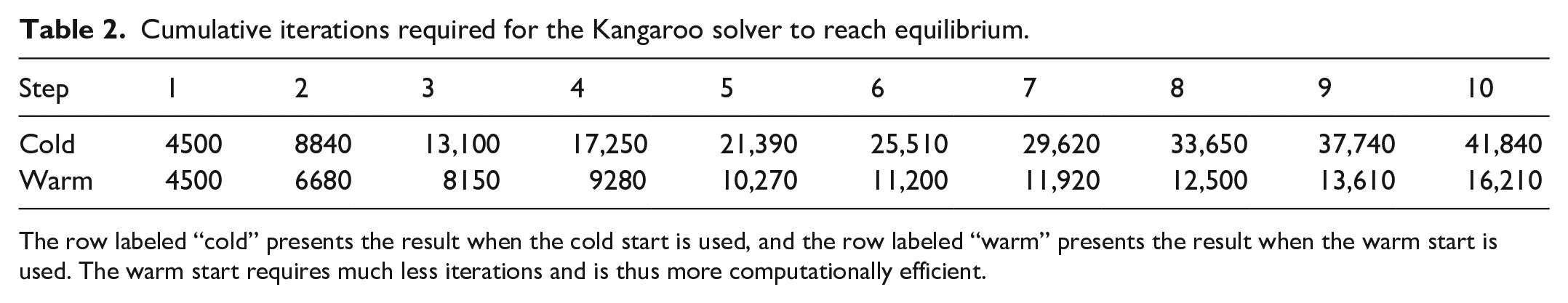
The row labeled “cold” presents the result when the cold start is used, and the row labeled “warm” presents the result when the warm start is used. The warm start requires much less iterations and is thus more computationally efficient.

Next, the mechanical property of the shape is compared to a benchmark shape, as shown in Figure 7. The benchmark shape is generated by discretizing the surface that directly interpolates the locations of pin-supports and target points so that the planar positions of the nodes are the same as the shape generated by the proposed method. Therefore, the only distinguishing factor between the two surfaces is the nodal heights. The structural analysis is carried out using Karamba.³⁶

Figure 7.

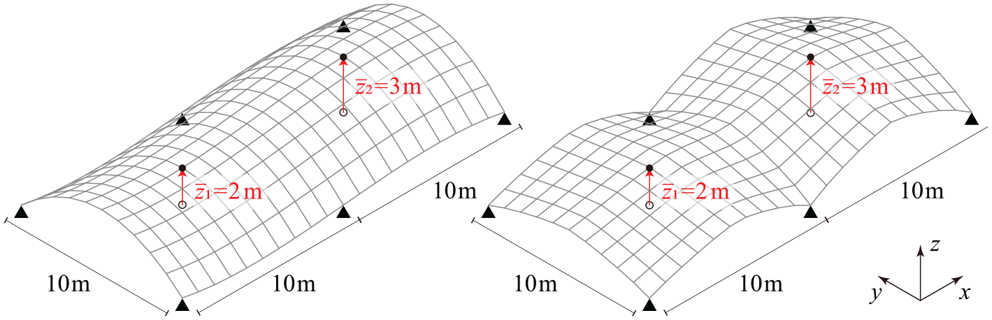
The benchmark surface interpolating the locations of pin-supports and target points (left) and the surface generated by the proposed method (right).

Figures 8 and 9 show the displacements and utilization factors of single-layered latticed shells where beam elements are arranged at each edge of the mesh and a downward load of 1.5 kN/m² has been applied. Steel is assumed as the material of the beams; Young’s modulus, the shear modulus, and the yield strength are 210,000, 80,760, and 235 N/mm², respectively. The beams have a uniform pipe cross-section with an external diameter of 140 mm and a thickness of 5 mm. Even though the proposed method designs a funicular shape for uneven load distribution, the shape also withstands a uniformly distributed vertical load with lower stresses. Table 3 shows the displacements and stresses under uniformly distributed loads. The deformation under vertical and horizontal loads can be suppressed in a well-balanced manner by generating the shape using the proposed method.

Figure 8.

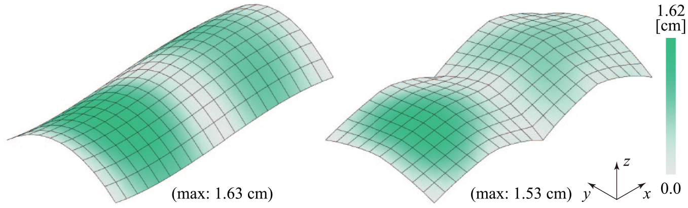
Displacements of steel latticed shells under a downward load of 1.5 kN/m².

Figure 9.

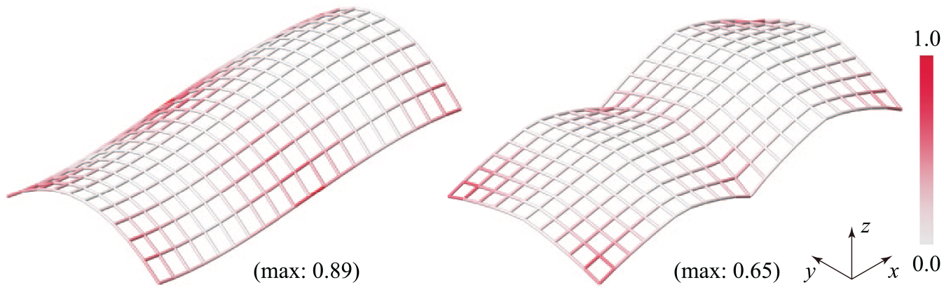
Utilization factors of steel latticed shells under a downward load of 1.5 kN/m².

Table 3.

The displacements and stresses of the benchmark shape and the shape generated by the proposed method under uniformly distributed loads.

Load	Benchmark	Proposed method
$1.0 kN / m^{2} (x)$
Displacement (cm)	$\sim 0.41$	$\sim 0.80$
Stress (N/mm²)	$- 59.0 \sim 59.4$	$- 56.7 \sim 50.7$
$1.0 kN / m^{2} (y)$
Displacement (cm)	$\sim 1.88$	$\sim 0.89$
Stress (N/mm²)	$- 139.1 \sim 136.7$	$- 74.3 \sim 74.5$
$- 1.5 kN / m^{2} (z)$
Displacement (cm)	$\sim 1.63$	$\sim 1.53$
Stress (N/mm²)	$- 155.7 \sim 130.0$	$- 121.0 \sim 114.7$

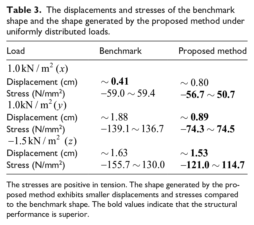
The stresses are positive in tension. The shape generated by the proposed method exhibits smaller displacements and stresses compared to the benchmark shape. The bold values indicate that the structural performance is superior.

We further investigate the effect of parameters ${\bar{z}}_{2}$ and $β$ on the shell geometry while fixing ${\bar{z}}_{1}$ to $2.0 m$ . Figure 10 illustrates the funicular shapes and the loads corresponding to various combinations of ${\bar{z}}_{2}$ and $β$ . From these results, the load distribution can be interpreted as the rationality of the target point locations. For example, the load direction flips when ${\bar{z}}_{2}$ is too small, indicating that the resulting shape may not withstand uniform vertical loads. In addition, it can be seen that smaller $β$ leads to a more uniform load distribution. Conversely, assigning a large value to $β$ yields a load distribution concentrated around the target points. One can play with the value of $β$ within a certain range for design exploration.

Figure 10.

Funicular shapes and loads for which the shapes are funicular.

Large-scale mesh with complex topology

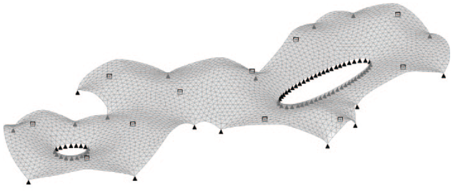
In this section, the method is applied to a more complex and large-scale model, as shown in Figure 11. This triangular mesh contains 2695 vertices and 5069 edges, and the height of the 11 target points are all 5 m. For this more challenging case, funicular shapes passing through multiple target points could be obtained, as shown in Figures 12 and 13. The RMSE regarding the target shape accuracy has been steadily reduced: 19.2 cm after 10 steps, 4.1 cm after 20 steps, and 1.1 cm after 30 steps.

Figure 11.

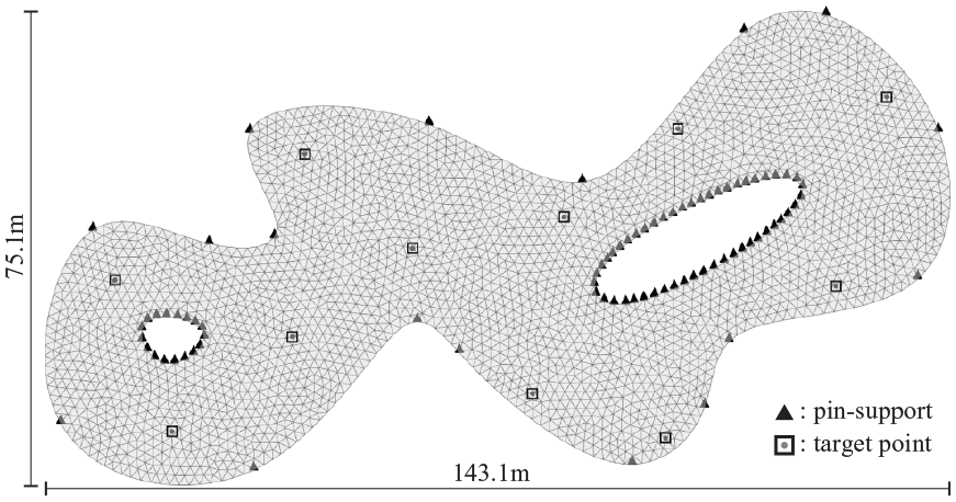
Plan view of the large-scale model.

Figure 12.

The shape of the large-scale model after applying the proposed method for 30 steps ( $β = 0.1$ , $RMSE = 1.1$ (cm)).

Figure 13.

Bird’s eye view of the nodal load vectors for which the shape in Figure 12 is funicular.

Conclusion

This study proposed a method to generate a funicular surface that passes through the user-specified target points. Instead of controlling the surface shape, this method controls the load distribution to deform a particle spring system to the target shape. An approach similar to gradient-based optimization was adopted to modify the load distribution to minimize the error between the current and target shapes. The approach includes a coarse line search and a warm start to improve the convergence property, and the whole process is encapsulated as a user-friendly tool that works in the Grasshopper© environment.

The validity of the proposed method has been demonstrated by the numerical examples. For a small-scale model, we investigated the effect of the coarse line search and the warm start. We verified that the coarse line search successfully determined approximately optimal step size regardless of the scale of the structure. We also verified that the warm start saves 61% of iterations compared with the cold start for the first 10 steps, and the saving rate becomes even higher as the step increases. Moreover, for a larger-scale model with thousands of nodes, the method successfully generated network surfaces that interpolate the prescribed target points at very high accuracy. Although the resulting shapes are funicular for non-uniform load distributions, the degree of load non-uniformity clearly informs the users of how rational the target point locations were against uniform vertical loads.

As explained above, this method prioritizes shape specification rather than structural rationality. Nevertheless, considering that the structural optimality is not necessarily equivalent to the design optimality, the developed method has the potential as a design exploration tool for non-engineering sectors, where playing with the target points yields a variety of shapes and the loads that the shapes are funicular for.

Footnotes

Declaration of conflicting interests

The author(s) declared no potential conflicts of interest with respect to the research, authorship, and/or publication of this article.

Funding

The author(s) received no financial support for the research, authorship, and/or publication of this article.

ORCID iD

Kazuki Hayashi

Code availability

The codes to reproduce the results presented in this paper are available at the following link: https://github.com/kazukihayashi/RBF_Load. The developed Grasshopper© component is available at the following link: .

This research received no specific grant from any funding agency in the public, commercial, or non-profit sectors. We would like to express our sincere gratitude to Daniel Piker, a developer of the Kangaroo library, for his valuable comments on distributing our tool.

References

Cowan

Domes: ancient and modern. J R Soc Arts 1983; 131(5320): 181–198. https://www-jstor-org-443.web.bisu.edu.cn/stable/41373544

Kampas

Kalapodis

McLean

, et al. Limit-state analysis of parabolic arches subjected to inertial loading in different gravitational fields using a variational formulation. Eng Struct 2021; 228(111501): 1–20. DOI: 10.1016/j.engstruct.2020.111501

Block

Ochsendorf

Thrust network analysis: a new methodology for three-dimensional equilibrium. J Int Assoc Shell Spatial Struct 2007; 48(3): 167–173.

Block

Thrust Network Analysis: Exploring three-dimensional equilibrium. PhD Thesis, Massachusetts Institute of Technology, UK, 2009.

Rippmann

Lachauer

Block

Interactive vault design. Int J Space Struct 2012; 27(4): 219–230.

Rippmann

Block

Funicular shell design exploration. In: Mungan

Abel

(eds.) Proceedings of the 33rd Annual Conference of the Association for Computer Aided Design in Architecture (ACADIA). Cambridge, ON, Canada: The Association for Computer Aided Design in Architecture (ACADIA), 2013, pp. 337–346.

Harding

Shepherd

Structural form finding using zero-length springs with dynamic mass. In: Mungan

Abel

(eds.) Proceedings of the IASS annual symposium. London: International Association for Bridge and Structural Engineering (IABSE) and International Association for Shell and Spatial Structures (IASS), 2011.

Harding

Lewis

The TRADA pavilion – a timber plate funicular shell. In: Obrębski

Tarczewski

(eds) Proceedings of the IASS annual symposium. Wroclaw University of Technology. Poland: International Association for Shell and Spatial Structures (IASS), 2013.

Bruggi

A constrained force density method for the funicular analysis and design of arches, domes and vaults. Int J Solids Struct 2020; 193–194(1): 251–269.

10.

Schek

HJ.

The force density method for form finding and computation of general networks. Comput Methods Appl Mech Eng 1974; 3(1): 115–134.

11.

Michiels

Adriaenssens

Dejong

Form finding of corrugated shell structures for seismic design and validation using non-linear pushover analysis. Eng Struct 2019; 181: 362–373.

12.

Kilian

Ochsendorf

Particle-spring systems for structural form finding. J Int Assoc Shell Spatial Struct 2005; 46(2): 77–84. https://www.ingentaconnect.com/contentone/iass/jiass/2005/00000046/00000002/art00003. (accessed 31 January 2024).

13.

Piker

Kangaroo: Form finding with computational physics. Archit Des 2013; 83(2): 136–137.

14.

Tamplin

Iuorio

. (2018) Challenges in designing and fabrication of a thin concrete shell. In: Mueller

Adriaenssens

(eds.) Proceedings of the IASS annual symposium. Boston, MA: International Association for Shell and Spatial Structures (IASS).

15.

Álvarez

Bernal

Design spaces of structurally pre-evaluated funicular shapes. In: Gomez

Braida

(eds) Proceedings of XXV International Conference of the Iberoamerican Society of Digital Graphics, vol. 9, 2021, pp.807–878, São Paulo, Brazil: Blucher.

16.

Capone

Lanzara

Portioli

FPA

, et al. Digital form finding using Voronoi pattern. Nexus Netw J 2021; 23(4): 959–975.

17.

Pugnale

Sassone

Morphogenesis and structural optimization of shell structures with the aid of a genetic algorithm. J Int Assoc Shell Spatial Struct 2007; 48: 161–166. https://www.ingentaconnect.com/content/iass/jiass/2007/00000048/00000003/art00010 (accessed 31 January 2024).

18.

Mueller

Ochsendorf

JA.

Combining structural performance and designer preferences in evolutionary design space exploration. Autom Constr 2015; 52: 70–82.

19.

Winslow

Multi-criteria gridshell optimization. In: Adriaenssens

Block

Veenendaal

, et al. (eds) Shell structures for architecture – form finding and optimization. London: Routledge, 2014, pp.181–193.

20.

Cui

Ohsaki

Shape design of curved surface of membrane structure using developable surface. J Int Assoc Shell Spatial Struct 2018; 59: 199–214.

21.

Barnes

MR.

Form finding and analysis of tension structures by dynamic relaxation. Int J Space Struct 1999; 14(2): 89–104.

22.

Kimura

Ohmori

Computational morphogenesis of free form shells. J Int Assoc Shell Spatial Struct 2008; 49(3): 175–180. https://www.ingentaconnect.com/content/iass/jiass/2008/00000049/00000003/art00011 (accessed 31 January 2024).

23.

ALGLIB®. Bicubic interpolation/fitting. https://www.alglib.net/interpolation/bicubic-spline-interpolation-fitting.php (accessed 23 November 2023).

24.

Hastie

Tibshirani

Friedman

2009. The Elements of Statistical Learning – Data Mining, Inference, and Prediction, chapter 5. 2nd ed. New York: Springer, 2009, pp. 144–146.

25.

Shepard

. (1968) A two-dimensional interpolation function for irregularly-spaced data. In: Proceedings of the 1968 23rd ACM National Conference, ACM ’68, 1968, pp. 517–524. New York, NY: Association for Computing Machinery. DOI:10.1145/800186.810616.

26.

Suominen

Tolvanen

Kalliola

Surface layer salinity gradients and flow patterns in the archipelago coast of SW Finland, northern Baltic Sea. Mar Environ Res 2010; 69(4): 216–226.

27.

Stachelek

Madden

CJ.

Application of inverse path distance weighting for high-density spatial mapping of coastal water quality patterns. Int J Geogr Inf Sci 2015; 29(7): 1240–1250.

28.

Nusret

Dug

. Applying the inverse distance weighting and kriging methods of the spatial interpolation on the mapping the annual precipitation in Bosnia and Herzegovina. In: Seppelt

Voinov

Lange

, et al. (eds.) Proceedings of the International Congress on Environmental Modelling and Software Managing Resources of a Limited Planet. Leipzig, Germany: International Environmental Modelling and Software Society (iEMSs), 2012.

29.

Wang

, et al. An adjusted inverse distance weighted spatial interpolation method. In: Proceedings of the 2018 3rd International Conference on Communications, Information Management and Network Security (CIMNS 2018), 2018, pp. 128–132. Wuhan, China: Atlantis Press.

30.

Cressie

Statistics for spatial data. Hoboken, NJ: Wiley, 1993.

31.

Sakata

Ashida

Zako

Structural optimization using kriging approximation. Comput Methods Appl Mech Eng 2003; 192(7–8): 923–939.

32.

Lee

Park

GJ.

A global robust optimization using kriging based approximation model. JSME Int J Ser C Mech Syst Mach Elem Manuf 2006; 49(3): 779–788.

33.

Jones

Schonlau

Welch

Efficient global optimization of expensive black-box functions. J Glob Optim 1998; 13: 455–492.

34.

Jin

Chen

The use of metamodeling techniques for optimization under uncertainty. Struct Multidiscipl Optim 2003; 25: 99–116.

35.

Bagheri

Konen

Bck

Comparing kriging and radial basis function surrogates. In: Workshop computational intelligence, 2017, pp. 243–259. Dortmund, Germany.

36.

Preisinger

Linking structure and parametric geometry. Archit Des 2013; 83: 110–113.