A Bayesian Optimal Foraging Model of Human Visual Search

Abstract

Real-world visual searches often contain a variable and unknown number of targets. Such searches present difficult metacognitive challenges, as searchers must decide when to stop looking for additional targets, which results in high miss rates in multiple-target searches. In the study reported here, we quantified human strategies in multiple-target search via an ecological optimal foraging model and investigated whether searchers adapt their strategies to complex target-distribution statistics. Separate groups of individuals searched displays with the number of targets per trial sampled from different geometric distributions but with the same overall target prevalence. As predicted by optimal foraging theory, results showed that individuals searched longer when they expected more targets to be present and adjusted their expectations on-line during each search by taking into account the higher-order, across-trial target distributions. However, compared with modeled ideal observers, participants systematically responded as if the target distribution were more uniform than it was, which suggests that training could improve multiple-target search performance.

Keywords

visual search environmental effects

When should a radiologist stop searching for abnormalities in your X-rays? How long should an airport baggage screener search through your luggage? When should a soldier stop looking for enemy combatants in a crowded town square? Furthermore, how should these policies be modified after a target is found? Searching for important objects in clutter is a ubiquitous real-world task and has been systematically studied in an effort to uncover the mechanisms of visual attention (see Eckstein, 2011; Nakayama & Martini, 2011, for recent reviews). Most prior research has used visual search as a tool to study visual attention and has focused on searches for a single target; however, some of the most important real-world visual search tasks, such as those conducted by radiologists, baggage screeners, and military personnel, are multiple-target searches that may contain many targets in a single display. For example, a medical X-ray scan can contain an unknown and unbounded number of potential abnormalities. This presents an interesting problem to the searcher—when to stop searching.

When searching for multiple targets, people are prone to overlook some of them (resulting in miss errors). Specifically, searchers are vulnerable to satisfaction-of-search errors (Tuddenham, 1962), in which targets that would likely be spotted in a single-target display are missed in a multiple-target display. Satisfaction-of-search errors may account for nearly 40% of misses in radiology (see Berbaum, Franklin, Caldwell, & Schartz, 2010, for a review) and are exacerbated by searcher anxiety (Cain, Dunsmoor, LaBar, & Mitroff, 2011). One can minimize miss errors by exhaustively inspecting every potential target; however, exhaustive search is prohibitively costly and inefficient in most situations, so usually searchers must stop without thoroughly inspecting every element of the display. Consequently, when the number of targets is unknown, efficient search requires tailoring a stopping decision to the distribution of targets across displays.

Prior evidence suggests that people adjust their search behavior on the basis of some aspects of the target distribution. Even in single-target search, target prevalence influences decision criteria, resulting in more false alarms (i.e., incorrect reports that a target is present) when targets are common and more misses when they are uncommon (Godwin et al., 2010; Wolfe et al., 2007; Wolfe & Van Wert, 2010). Similarly, in multiple-target search, errors are influenced by the base rates of specific targets, with less-frequent targets missed more often than more-frequent targets (e.g., Fleck, Samei, & Mitroff, 2010). It is important to note that these prevalence effects are driven implicitly by experience with particular search environments rather than explicitly by top-down expectations, such as instructions (Lau & Huang, 2010). These data suggest that human search behavior adjusts to environmental statistics, but they raise a number of important questions for real-world search: Are these adaptations appropriate for the learned statistics of the search displays? How sophisticated are the environmental statistics used to guide search strategies? Finally, how do people use these statistics to decide when to stop searching when the number of targets is unknown?

Although the effects of the search environment have not been well explored in humans, there is an extensive literature on animal foraging that has formalized how nonhumans make use of the statistical properties of their environments (see Stephens & Krebs, 1986, for a review). Optimal foraging theory provides a rational analysis of the behavior of animals consuming food from a number of “patches,” formally answering questions such as “When should a blue jay stop eating from one cherry tree and move to another?” The key insight of optimal foraging theory is that an organism should strive to maximize its rate of energy intake, rather than, say, ensuring that it has consumed all available food. Thus, an organism should leave one location and move to the next when the instantaneous rate of energy intake for the current location falls below the expected rate for the environment as a whole. In short, a forager should aim to spend time in locations with above-average quantities of food and leave them once those quantities drop below average. This model has been applied almost exclusively to analyze animal behavior, but some work suggests that human behaviors may follow similar patterns (e.g., Hutchinson, Wilke, & Todd, 2008; Pirolli, 2007). In the current study, we presented people with complexly structured search environments and evaluated how well they adapted to them by comparing their behavior with that of an optimal foraging model instantiating Bayesian learning.

Method

In this study, we investigated whether human observers adjusted their search strategies in response to complex target-distribution statistics. Participants searched for T-shaped targets among pseudo-L-shaped distractors (Fig. 1) and were awarded 15 points for each target found, with the experiment ending when they accumulated 2,000 points. There were no penalties for misses or false alarms. Participants were assigned to three different groups, with each group observing different distributions of the number of targets present per display; crucially, the overall target prevalence (Wolfe et al., 2007) was matched across conditions: one target per trial, on average. The number of targets on each target-present trial was sampled from a geometric distribution, with the rate parameter adjusted to yield this overall prevalence; however, we manipulated the rate at which target-present trials occurred. In the 25% condition, only one quarter of the trials had at least one target, but those trials were likely to contain many targets. In the 50% condition, half of the trials had at least one target, and of those trials, half had one target and half had more than one. In the 75% condition, three quarters of the trials had at least one target, but those trials were unlikely to contain more than one target. Did people adjust their search strategies based on these target distributions?

Fig. 1.

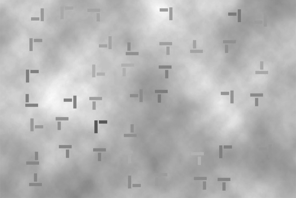
Sample search array used in the experiment. Stimuli consisted of pairs of rectangles, with the members of each pair oriented perpendicularly to each other to form perfect T shapes (targets) or pseudo-L shapes (distractors). All displays contained 40 items (27%–65% black), 0 to 12 of which were targets (6 are present in this example). Stimuli were presented on a background of gray-scale “clouds.”

Participants and conditions

Sixty-two members of the Duke University community participated for partial fulfillment of a course requirement or a $10 payment. Nine participants were excluded for failing to complete the experiment in less than 75 min,¹ and a further 8 participants were excluded for making false alarm responses on 25% or more of the trials. There was no difference in the number of excluded participants across conditions, χ²(2, N = 17) = 2.22, p = .329. The remaining 45 participants (17 males and 28 females) ranged in age from 18 to 48 years (median = 23).

Each participant was randomly assigned to one of three between-participants conditions that differed in the number of trials containing targets but with the expected number of targets per trial held constant (Fig. 2). In the 25% condition, only one quarter of the trials had one or more targets. In the 50% condition, half of the trials had one or more targets. In the 75% condition, three quarters of the trials had one or more targets. The number of targets on each target-present trial was sampled from a geometric distribution, with the rate parameter adjusted per condition to yield the same overall average of one target per trial. In the 25% condition, there were a maximum of 12 targets per trial. In the 50% condition, up to 8 targets per trial were presented in the display, and in the 75% condition, there were up to 4 targets per trial. These target distributions provided complex, but informative, target-prevalence statistics.

Fig. 2.

Distribution of the number of targets present in each display in the three conditions. In all conditions, the expected number of targets per trial was one, but the proportion of trials with targets differed across conditions.

Procedure

Stimuli were presented on Dell Inspiron computers with 20-in. CRT monitors and were programmed in MATLAB (The MathWorks, Natick, MA) using the Psychophysics Toolbox (Version 3.0.8; Brainard, 1997; Kleiner, Brainard, & Pelli, 2007; Pelli, 1997). Observers were seated approximately 50 cm from the screen. Each trial began with a black 1.5° × 1.5° fixation cross, which appeared for 0.5 s at the center of a white screen. The cross was replaced with a search array of 40 pairs of gray rectangles (27%–65% black; Fig. 1). Each pair was contained within an invisible 1.3° × 1.3° square. The members of each pair were oriented perpendicularly to each other and slightly separated. Targets were perfect T shapes, and distractors were pseudo-L shapes. Targets and distractors were randomly positioned within the search array. The search array was presented on a background of gray-scale “clouds” (4%–37% black). Intertrial intervals lasted 3 s each.

Participants were awarded 15 points for each target found, with the experiment ending when they reached 2,000 points, that is, 134 found targets. These values were selected based on pilot testing so that an experimental session was expected to last just under 1 hr, with participants taking 54 min, on average. There were no penalties for misses or false alarms. Participants made a localization mouse click on each target they found (which was then marked with a small 0.2° × 0.2° blue circle). Once they decided to terminate a search, they clicked a button labeled “Done” to end that trial. A 3-s feedback screen after each trial revealed all the targets that were present to provide all participants with the same information about the target distribution regardless of their performance. The experiment began with a practice block that had a 120-point goal to familiarize participants with the target distribution in their conditions.

Results

Participants produced false alarms on 6.14% of trials, with no difference in false alarm rates among conditions, F(2, 42) = 0.38, p = .684; these trials were excluded from further analyses. Overall, 26.39% of all targets were missed, again with no differences between conditions, F(2, 42) = 1.86, p = .168. These metrics suggest that overall search dynamics were comparable across conditions.

Although coarse search behavior was similar across distribution conditions, adjusting to these distributions predicted fine-grained differences in the search dynamics. Specifically, we were interested in how long it took the participants to decide to stop searching: How long did they search after finding the last target on a trial (even if not all targets were found)? We operationalized this question as the time between the last click on a target and a click on the “Done” button. Figure 3a plots this difference measure against the number of targets found in each condition. The main pattern is clear: The more targets that were likely to be in a display, the longer participants continued searching before terminating their search. This was confirmed with a 3 × 4 mixed model analysis of variance (ANOVA) with condition (25%, 50%, or 75%) and number of targets found (0, 1, 2, or 3) as factors.² There were significant main effects of condition, F(2, 126) = 4.86, p = .013, and of number of targets found, F(3, 126) = 161.48, p < .001, and a significant interaction between these factors, F(6, 126) = 5.08, p < .001.

Fig. 3.

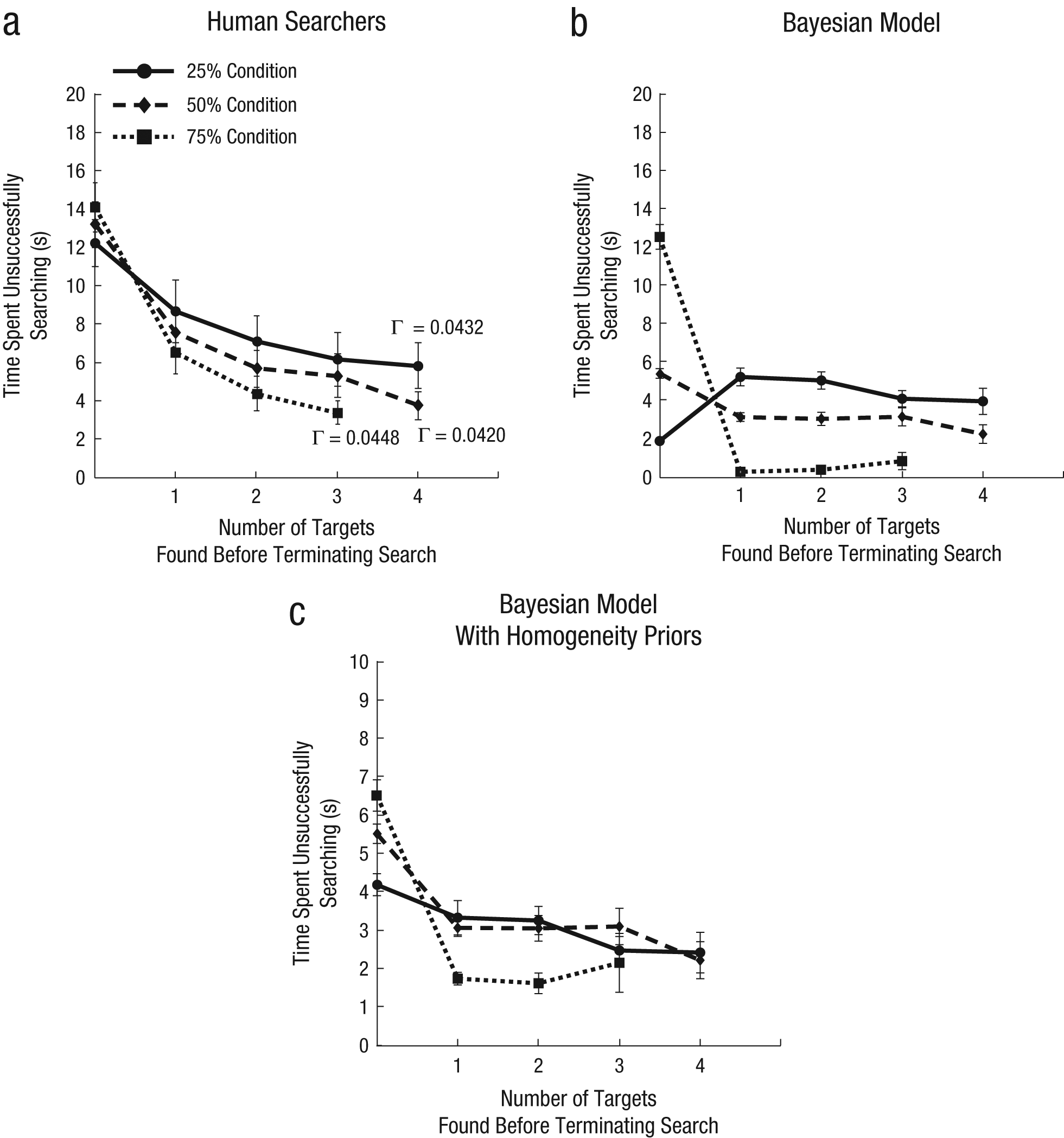
Time spent unsuccessfully searching for an additional target as a function of the number of targets found before terminating the search in each condition. The graphs show (a) behavioral results (with expected values expressed in targets per second), (b) results for an ideal observer derived from a Bayesian optimal foraging model, and (c) results from the Bayesian model including participants’ prior expectations that targets tend to appear on about half of the trials and tend to be distributed homogeneously. The value for four targets is not plotted for the 75% condition, as fewer than half the participants in this condition found four targets in a single display. Error bars show standard errors of the mean.

This interaction reveals a number of key features: When no targets had been found, participants searched longer if they were in a condition in which trials were more likely to have at least one target than did participants in conditions in which trials with targets occurred less often (i.e., 75% condition > 50% condition > 25% condition, which is a significant linear trend), F(1, 42) = 5.54, p = .023. However, once a single target was found, the pattern reversed: Participants in conditions in which target displays tended to contain more targets searched for a second target longer than did participants in conditions in which multiple-target trials were rarer (i.e., 25% condition > 50% condition > 75% condition); significant linear trends for one, two, and three targets were found across conditions (all ps < .02). This pattern also held for two, three, and four targets found.

Overall rate of target finding

We assume searchers aim to maximize Γ, their rate of finding targets across the whole experiment (thus, minimizing the total time to accumulate 2,000 points and finish the experiment), which can be represented by the following formula:

Γ = \frac{\bar{n}}{\bar{t} + τ},

where $\bar{n}$ is the average number of targets found per trial, $\bar{t}$ is the average time spent searching per trial, and τ is the constant intertrial interval (3 s in the current experiment). A higher Γ indicates that a searcher spent less time searching unrewarding displays and more time searching displays with many targets.

We calculated Γ for each searcher. A one-way ANOVA with condition (25%, 50%, or 75%) as a factor revealed that Γ did not differ among distribution conditions (25% condition: Γ = 0.045 ± 0.008 targets/s, 50% condition: Γ = 0.042 ± 0.006 targets/s, 75% condition: Γ = 0.044 ± 0.010 targets/s), F(2, 42) = 0.44, p = .647. This null effect reflects both a lack of differences in $\bar{n}$ and a lack of differences in $\bar{t}$ : Participants found an average of 0.78 targets per display and spent an average of 14.47 s searching each display, with no differences between groups on either measure, F(2, 42) = 0.94, p = .398, and F(2, 42) = 0.08, p = .926, respectively. Thus, despite searching under different target distributions, each group settled on the same average target-acquisition rate (both finding similar numbers of targets and taking the same overall time to do so), a behavior that could arise only if searchers were adapting their behavior to the statistics of their search environment.

Bayesian optimal foraging model

We modeled participants’ decisions to continue searching any one display in our experiment using the optimal foraging model that is used to describe how, for example, blue jays choose whether to continue foraging a given cherry tree. Specifically, the marginal value theorem (Charnov, 1976) predicts that an optimal forager should abandon a search at its current location when the instantaneous rate of return of the current location reaches the overall rate of return for the environment. This principle predicts behavior across a wide range of species, including parasitic insects (Wajnberg, Fauvergue, & Pons, 2000), rats (Mellgren, 1982), birds (Ydenberg, 1984), and monkeys (Hayden, Pearson, & Platt, 2011). However, the marginal value theorem does not perform well when locations may contain only a few targets, as was the case in our experiment (Biernaskie, Walker, & Gegear, 2009; McNamara, Green, & Olsson, 2006). For this reason, we employed the potential value theorem (McNamara, 1982; Olsson & Brown, 2006), which extends the marginal value theorem to such discrete cases by positing that foragers leave their current location when the predicted value of staying is less than the predicted value of searching a new location. Such a forager updates its value prediction for the current location at each point in time, noting how much time was spent searching and how many targets were found. We implemented this prediction of value via a Bayesian ideal observer sensitive to the across-trial target distribution.

Bayesian potential value estimation

Under the potential value theorem, searchers should calculate the potential value of the current display, Π. With small numbers of targets, each of which is found independently, Π is the ratio of the expected probability of the next item searched being a target and the time it will take to search that additional item. When Π falls below Γ, the searcher should move on to a new display. To calculate Π, we used a Bayesian ideal observer that starts every trial with a prior over the total number of targets, p(T), which reflects the learned distribution of targets across displays. Then the ideal observer computes the posterior probability of the total number of targets, p(T|F, S), after having found F targets having searched S items on this display: p(T|F, S) ∝ p(F|T, S)p(T).

The likelihood, p(F|T, S), reflects a process of randomly sampling items from the display while replacing distractors but without replacing targets: When a target is found, it cannot be marked again, but when a distractor is found, it continues to be sampled during the rest of the search (Horowitz & Wolfe, 2001).³ For example, in searching for 5 targets among 40 items, the probability of finding a target is 5/40 on each draw until the first target is found, then the probability of finding the second target on subsequent draws becomes 4/39, and so forth. The pseudo-hypergeometric distribution that results from such partial replacement has no analytical form, but it can be numerically calculated with high precision for the range of F, S, and T values we used here.

Using the posterior probability of T, p(T|F, S), and the number of items in the display, N (always 40), we calculated the expected probability of the next sampled item being a target by marginalizing over T:

E [\frac{T - F}{N - F} | F, S] = \sum_{T} \frac{T - F}{N - F} P (T | F, S),

and thus calculated Π as follows:

Π = \frac{E [\frac{T - F}{N - F} | F, S]}{γ},

where γ is the time it takes to search one more item.

We ran the model on the specific time courses and trials of each participant in each condition; thus, we could predict stopping times for every trial that went into our empirical averages. For each trial, we considered the point when the last target was found (or the start of the trial on trials where no targets were found) and calculated Π in 500-ms intervals from that point. Thus, we could determine when Π, as calculated by the ideal observer, would fall below that participant’s empirical value of Γ. We took the point at which this happened as the stopping time for the ideal observer. These calculations were predicated on the conversion of the number of items searched to time by assuming that each item took 250 ms to search—this value was based on search slope measures obtained in a supplement experiment (see the Supplemental Material available online).

Figure 3b shows that the model captured the major qualitative features of human behavior in our search task. When no targets have been found, searchers in the 75% condition have cause for optimism and would be expected to search for a long time before stopping; in contrast, searchers in the 25% condition should be pessimistic about the prospects of the display containing any targets at all. However, once a target has been found, these expectations reverse: Searchers in the 75% condition should not expect to find any more targets, and observers in the 25% condition should expect to find many more. This should result in observers in the 25% condition searching longer for subsequent targets. The model searched longer in the 75% condition than in the 25% condition when no targets had been found, and importantly, this relationship reversed when one or more targets had been found. In the 25% condition, when most trials did not contain targets, the model correctly interpreted the first target as good news (Olsson & Brown, 2006) and persevered in searching for additional targets. However, in the 75% condition, finding the first target indicated that few additional targets remained, so there was little point in searching for them.

Although the ordering of conditions corresponded well to the order of behavioral results, there was a striking difference between the magnitude of the actual and modeled searching times when no targets had been found in the 25% and 75% conditions. This suggests that participants in those conditions were taking a conservative approach to target-absent trials by spending almost as much time searching on those trials as they did on average across the experiment rather than fully adjusting to the environmental search statistics. In contrast, for the 50% condition, the model and the empirical search data aligned quite well when no targets have been found. This suggests that searchers may not be effectively learning the proportion of trials that do and do not have targets and thus may be acting as if the prevalence of trials with targets is close to 50% when no target has been found. However, they may be better able to learn the distribution of targets in target-present trials.

Prior expectations about target distributions

Although human behavior qualitatively matched that of the ideal observer, the quantitative effects predicted by our model were far larger than those shown in the behavioral results. Such a difference would naturally arise if participants came into our experiment expecting a relatively homogeneous distribution of targets across displays. To capture such an expectation, we added priors to our model favoring homogeneity, with two parameters corresponding to the strength of the prior favoring a 50% chance of a target-present trial and the strength of the prior favoring a 0.5 geometric-rate parameter. We formalized the prior over target-present trials as a beta distribution over the probability that a display contains a target (with parameters α = 0.5 × θ, β = 0.5 × θ); thus, θ corresponds to the strength of the prior favoring a 50% chance of a target-present display, intuitively interpreted as the number of displays that had been previously seen with 50% target prevalence.

We also included a beta prior on the geometric-rate parameter describing the number of targets in a display, also favoring a rate parameter of 0.5 (reflecting an expected value of two targets per target-present display) and parameterized by λ, which corresponds intuitively to the number of target-present trials previously seen with that rate parameter. Using these parameters, we could estimate the strength of the homogeneity priors that best describe the overall group performance. The values we found (θ = 519 and λ = 296) indicate that participants seemed to have a stronger expectation that roughly 50% of trials ought to contain targets, as compared with their expectation about the number of targets on target-present trials.

Figure 3c shows model predictions using this best-fitting prior. Without this prior expectation, the correlation among model predictions and stopping times on individual trials across all participants and conditions was .42 (r² = .17; n = 7,473 trials). By adding the homogeneity priors, the correlation significantly improved (r = .59, r² = .34; Fisher Z = 14.1, p < .001). This improvement suggests that participants came to the present experiment with an expectation of 50% target prevalence and an even target distribution. To convey how much of an effect this prior had, we can estimate the parameters that participants must have learned by the end of the experiment. We found that for the 25%, 50%, and 75% conditions, respectively, participants learned that the average rates of targets per trial were 0.44, 0.50, and 0.57, and that the geometric-rate parameters were 0.42, 0.50, and 0.60. The fact that the 50% condition matched this homogeneous prior expectation may explain the greater correspondence in this condition between behavior and modeled performance without the homogeneity prior.

General Discussion

The results of the present experiment demonstrate that searchers can adapt to complex statistics of their search environment in sophisticated ways: Participants terminated their searches quickly when the presence of an additional target was unlikely but searched longer when finding an additional target was more likely. This was observed both within participants (with a main effect of number of targets found) and between groups (with an interaction between condition and number of targets found), which suggests that people optimize their search strategies for their environment. Although the searchers in the 50% condition performed nearly optimally, searchers in the 25% and 75% conditions deviated from optimal predictions by not sufficiently adjusting to the target distributions.

Only one other study to date has examined sensitivity to patchy target distributions in a human visual cognition task: Hutchinson et al. (2008) presented participants with a simulated fishing task, in which fish appeared at a rate dependent on the number remaining in the pond. Participants could switch to a new pond at any time (with a fixed transition duration). The researchers found that participants generally responded appropriately when presented with clustered targets but dwelled longer than optimal on a given pond. Our fine-grained analysis showed deviations in both directions from optimality depending on the number of targets found and the target distribution: Although people adjust to the target distribution, they do not adjust as much as is optimal.

To date, no model of multiple-target visual search has been put forward to explain search-termination behavior. We propose that human visual search can be modeled in the same manner as foraging behavior in animals, which suggests a wealth of possibilities for future studies. Our experiment demonstrates that although searchers do not adjust their strategies as much as would be optimal, they are sensitive to the same factors used by the ideal observer model to determine stopping times. We suspect that the same strategic considerations underlying the behavior we observed likely account for target-prevalence effects (Wolfe & Van Wert, 2010) and satisfaction-of-search effects (Fleck et al., 2010) in visual search, with participants maximizing their rate of target finding on the basis of the statistics of the search environment. The generality of this mechanism has broad implications; for example, artificially modifying target-distribution statistics, such as priming baggage screeners with daily training runs of multiple-target bags (cf. Wolfe et al., 2007), may be an effective way to enhance sensitivity in critical multiple-target visual searches.

Footnotes

Acknowledgements

The authors thank Ricky Green and Elise Darling for help with participant testing, Ben Hayden and John Pearson for their thoughts on optimal foraging theory, Sasen Cain for modeling insight, and the Mitroff lab for helpful comments and feedback.

Declaration of Conflicting Interests

The authors declared that they had no conflicts of interest with respect to their authorship or the publication of this article.

Funding

This work was partially supported by the Army Research Office (Grant No. 54528LS) and partially supported through a subcontract with the Institute for Homeland Security Solutions, a research consortium sponsored by the Human Factors Division in the Department of Homeland Security (DHS). This material is based on work supported by the DHS under Contract No. HSHQDC-08-C-00100. Any opinions, findings, and conclusions or recommendations expressed in this material are those of the authors and do not necessarily reflect the official policy or position of DHS or of the U.S. government. This study is approved for public release.

Supplemental Material

Additional supporting information may be found at

Notes

References

Berbaum

K. S.

Franklin

E. A.

Caldwell

R. T.

Schartz

K. M.

(2010). Satisfaction of search in traditional radiographic imaging. In Samei

Krupinski

(Eds.), The handbook of medical image perception and techniques (pp. 107–138). Cambridge, England: Cambridge University Press.

Biernaskie

J. M.

Walker

S. C.

Gegear

R. J.

(2009). Bumblebees learn to forage like Bayesians. The American Naturalist, 174, 413–423.

Brainard

D. H.

(1997). The Psychophysics Toolbox. Spatial Vision, 10, 433–436.

Cain

M. S.

Dunsmoor

J. E.

LaBar

K. S.

Mitroff

S. R.

(2011). Anticipatory anxiety hinders detection of a second target in dual-target search. Psychological Science, 22, 866–871. doi:10.1177/095679761141239310.1177/0956797611412393

Charnov

(1976). Optimal foraging: The marginal value theorem. Theoretical Population Biology, 9, 129–136.

Eckstein

M. P.

(2011). Visual search: A retrospective. Journal of Vision, 11(5), Article 14. doi:10.1167/11.5.1410.1167/11.5.14

Fleck

M. S.

Samei

Mitroff

S. R.

(2010). Generalized “satisfaction of search”: Adverse influences on dual-target search accuracy. Journal of Experimental Psychology: Applied, 16, 60–71. doi:10.1037/a001862910.1037/a0018629

Godwin

H. J.

Menneer

Cave

K. R.

Helman

Way

R. L.

Donnelly

(2010). The impact of relative prevalence on dual-target search for threat items from airport X-ray screening. Acta Psychologica, 134, 79–84. doi:10.1016/j.actpsy.2009.12.00910.1016/j.actpsy.2009.12.009

Hayden

B. Y.

Pearson

J. M.

Platt

M. L.

(2011). Neuronal basis of sequential foraging decisions in a patchy environment. Nature Neuroscience, 14, 933–939. doi:10.1038/nn.285610.1038/nn.2856

10.

Horowitz

T. S.

Wolfe

J. M.

(2001). Search for multiple targets: Remember the targets, forget the search. Perception & Psychophysics, 63, 272–285.

11.

Hutchinson

J. M. C.

Wilke

Todd

P. M.

(2008). Patch leaving in humans: Can a generalist adapt its rules to dispersal of items across patches? Animal Behaviour, 75, 1331–1349. doi:10.1016/j.anbehav.2007.09.00610.1016/j.anbehav.2007.09.006

12.

Kleiner

Brainard

Pelli

(2007, August). What’s new in Psychtoolbox-3? Tutorial session presented at the 30th European Conference on Visual Perception, Arezzo, Italy.

13.

Lau

J. S.

Huang

(2010). The prevalence effect is determined by past experience, not future prospects. Vision Research, 50, 1469–1474. doi:10.1016/j.visres.2010.04.02010.1016/j.visres.2010.04.020

14.

McNamara

J. M.

(1982). Optimal patch use in a stochastic environment. Theoretical Population Biology, 21, 269–288. doi: 10.1016/0040-5809(82)90018-110.1016/0040-5809(82)90018-1

15.

McNamara

J. M.

Green

R. F.

Olsson

(2006). Bayes’ theorem and its applications in animal behaviour. Oikos, 112, 243–251. doi:10.1111/j.0030-1299.2006.14228.x10.1111/j.0030-1299.2006.14228.x

16.

Mellgren

R. L.

(1982). Foraging in a simulated natural environment: There’s a rat loose in the lab. Journal of the Experimental Analysis of Behavior, 38, 93–100. doi:10.1901/jeab.1982 .38-9310.1901/jeab.1982.38-93

17.

Nakayama

Martini

(2011). Situating visual search. Vision Research, 51, 1526–1537. doi:10.1016/j.visres.2010.09.00310.1016/j.visres.2010.09.003

18.

Olsson

Brown

J. S.

(2006). The foraging benefits of information and the penalty of ignorance. Oikos, 112, 260–273. doi:10.1111/j.0030-1299.2006.13548.x10.1111/j.0030-1299.2006.13548.x

19.

Pelli

D. G.

(1997). The VideoToolbox software for visual psychophysics: Transforming numbers into movies. Spatial Vision, 10, 437–442.

20.

Peterson

M. S.

Kramer

A. F.

Wang

R. F.

Irwin

D. E.

McCarley

J. S.

(2001). Visual search has memory. Psychological Science, 12, 287–292.

21.

Pirolli

(2007). Information foraging theory: Adaptive interaction with information. New York, NY: Oxford University Press.

22.

Stephens

D. W.

Krebs

J. R.

(1986). Foraging theory (1st ed.). Princeton, NJ: Princeton University Press.

23.

Tuddenham

W. J.

(1962). Visual search, image organization, and reader error in roentgen diagnosis: Studies of the psycho-physiology of roentgen image perception. Radiology, 78, 694–704.

24.

Wajnberg

Fauvergue

Pons

(2000). Patch leaving decision rules and the marginal value theorem: An experimental analysis and a simulation model. Behavioral Ecology, 11, 577–586. doi:10.1093/beheco/11.6.57710.1093/beheco/11.6.577

25.

Wolfe

J. M.

Horowitz

T. S.

Van Wert

M. J.

Kenner

N. M.

Place

S. S.

Kibbi

(2007). Low target prevalence is a stubborn source of errors in visual search tasks. Journal of Experimental Psychology General, 136, 623–638. doi:10.1037/0096-3445 .136.4.62310.1037/0096-3445.136.4.623

26.

Wolfe

J. M.

Van Wert

M. J.

(2010). Varying target prevalence reveals two dissociable decision criteria in visual search. Current Biology, 20, 121–124. doi:10.1016/j.cub.2009.11.06610.1016/j.cub.2009.11.066

27.

Ydenberg

R. C.

(1984). Great tits and giving-up times: Decision rules for leaving patches. Behaviour, 90(1/3), 1–24.

Supplementary Material

Please find the following supplemental material available below.

For Open Access articles published under a Creative Commons License, all supplemental material carries the same license as the article it is associated with.

For non-Open Access articles published, all supplemental material carries a non-exclusive license, and permission requests for re-use of supplemental material or any part of supplemental material shall be sent directly to the copyright owner as specified in the copyright notice associated with the article.

0.00 MB

0.07 MB