Time Order as Psychological Bias

Abstract

Incorrectly perceiving the chronology of events can fundamentally alter people’s understanding of the causal structure of the world. For example, when astronomers used the “eye and ear” method to locate stars, they showed systematic interindividual errors. In the current study, we showed that temporal-order perception may be considered a psychological bias that attention can modulate but not fully eradicate. According to Titchener’s law of prior entry, attention prioritizes the perception of an event and thus can help compensate for possible interindividual differences in the perceived timing of an event by normalizing perception in time. In a longitudinal study, we tested the stability of participants’ temporal-order perception across and within sensory modalities, together with the magnitude of the participants’ prior-entry effect. All measurements showed the persistence of stable interindividual variability. Crucially, the magnitude of the prior-entry effect was insufficient to compensate for interindividual variability: Conscious time order was systematically subjective, and therefore traceable on an individual basis.

Keywords

temporal order interindividual variability multisensory attention time consciousness open data

The perception of temporal order is seldom veridical (Sanford, 1888) and can be modulated by attention (Shore, Spence, & Klein, 2001; Spence, Shore, & Klein, 2001). According to Titchener’s law of prior entry (Titchener, 1908), a stimulus to which one pays attention will be systematically perceived before a stimulus that one ignores. The law of prior entry predicts that attention prioritizes the arrival time of sensory stimuli; thus, it may govern people’s subjective awareness of timing and may be instrumental in adjusting neural latencies across senses (Spence & Squire, 2003). Attention, temporal integration (Colonius & Diederich, 2004; van Wassenhove, Grant, & Poeppel, 2007), and active compensation (Sugita & Suzuki, 2003) can all contribute to even out the timing of sensory information in the brain, enabling multisensory integration. Yet even if integration yields to the compression of information in time and theoretically causes a loss of temporal resolution, the serial order of multisensory events in the few tens of milliseconds does not fully escape people’s consciousness (Efron, 1973; van Eijk, Kohlrausch, Juola, & van de Par, 2008). Researchers have observed high interindividual variability in temporal-order perception (Boenke, Deliano, & Ohl, 2009; Freeman et al., 2013; Kösem, Gramfort, & van Wassenhove, 2014; Sanford, 1888; Stone et al., 2001; Vroomen, Keetels, de Gelder, & Bertelson, 2004), which suggests that attention may not be fully sufficient to compensate for possible individual biases in order perception. To date, however, no studies have tackled this question.

In the current study, we sought to determine whether participants’ attentional state could fully account for interindividual variability in temporal-order perception. We used audiovisual temporal-order judgments, which allowed us to manipulate participants’ attention toward one sensory modality (i.e., hearing) or another (i.e., vision). In prior work on audiovisual temporal order, the researchers have either not explicitly controlled for cross-modal attention (Boenke et al., 2009; Vroomen et al., 2004; Zampini, Shore, & Spence, 2003) or have considered the prior-entry effect to be an index of temporal-order perception (Spence et al., 2001; Weiss, Hilkenmeier, & Scharlau, 2013).

We combined both approaches in the current study and assessed audiovisual temporal-order thresholds, or audiovisual points of subjective simultaneity (PSSs), with two experimentally independent measures. The first measure of audiovisual PSS was calculated during a condition in which attention was split between hearing and vision (split-attention PSS). The second measure of audiovisual PSS was computed using two experimental conditions, one manipulating attention toward hearing and the other manipulating attention toward vision, and these conditions provided the basis for a measure free of any attentional bias (bias-free PSS). To test the stability of individual temporal-order perception over time, we used a longitudinal approach and systematically estimated both PSSs over a 4-month period. Noel, Niear, Burg, and Wallace (2016) advocated the use of longitudinal approaches to establish the robustness of multisensory timing during the life span; to the best of our knowledge, only one study (Stone et al., 2001) has reported strong within-participant correlations of audiovisual simultaneity over a 1-week period, but there was a change of viewing distance between the two sessions. The stability of PSSs and the prior-entry effect could thus be tested, along with the relationship between the prior-entry effect (i.e., the effect of paying attention to one sensory modality or the other) and PSS (i.e., a measure of temporal-order perception independent of attention to one sensory modality or the other) at the individual level. The auditory and visual PSSs and spatial biases were also assessed as a result of the spatial nature of the task that was used.

Method

Participants

Twenty-four right-handed naive participants with normal or corrected-to-normal vision and normal hearing took part in the study (9 men and 15 women; mean age = 25 years, SD = 4). Each provided written informed consent in accordance with the Declaration of Helsinki (World Medical Association, 2013), and the study was approved by the human research ethics committee at NeuroSpin (Gif-sur-Yvette, France). Five participants were excluded because their PSSs were located outside the range of tested stimulus onset asynchronies, or SOAs (according to the criteria used in Spence et al., 2001). Thus, in the final analysis, we included 19 participants (7 men and 12 women; mean age = 25 years, SD = 4), well above the requirement of 13 participants suggested by a sample-size analysis using the ICC.Sample.Size package (Rathbone, Shaw, & Kumbhare, 2015) for the R software environment (Version 3.2.4; R Development Core Team, 2016). We used the following settings: α = .05, hypothesized value of ICC = .8, null-hypothesis value of ICC = .4, and power = .9. A post hoc power analysis revealed that our study had a power of .97 to detect the smallest ICC that we observed (.46), with α = .05 and a null hypothesis of ICC = 0 (i.e., no intraclass reliability).

Stimuli

The experiment was designed using Psychophysics Toolbox (Version 3.0.11; http://psychtoolbox.org/) and MATLAB (Version 2014a; The MathWorks, Inc., Natick, MA). The visual stimuli were white dots (luminance = 4 lux, diameter = 1.8°) presented for 35 ms (three frames) on a black CRT screen (refresh rate = 85 Hz, resolution = 1,024 × 728 pixels). The center of the dots was presented at an eccentricity of 14° of visual angle from the horizontal meridian. Auditory stimuli were sine-wave tones (2 kHz, 63 dB) presented for 35 ms (including 5-ms fade-in and 5-ms fade-out). Speakers were placed on each side of the monitor screen at 19° of eccentricity from the center of the screen on the horizontal meridian.

The stimuli were separated by 13 different SOAs, each of which was variable: 0 ms (SD = 3), 34 ms (SD = 4), –34 ms (SD = 4), 54 ms (SD = 7), –54 ms (SD = 7), 68 ms (SD = 5), –68 ms (SD = 5), 98 ms (SD = 6), –98 ms (SD = 6), 145 ms (SD = 7), –145 ms (SD = 7), 237 ms (SD = 5), and –237 ms (SD = 5). A negative value for delay indicates that the left stimulus was presented first, and a positive value indicates that the right stimulus was presented first. The synchronization and stability of stimulus timing was verified with an oscilloscope using a photodiode and a microphone. Each SOA was measured 18 times for each pair of visual stimuli (flashes; VV), each pair of auditory stimuli (sounds; AA), and each pair of audiovisual stimuli (a sound and a flash; AV). A mean standard deviation of 5 ms was observed across all conditions. To ensure that the variability in stimulus delivery would not affect the measurements of individual PSSs, we modeled the distribution of possible PSSs, taking into account this variability. For this analysis, one PSS was derived from simulated data in response to a set of 13 SOAs; each of the 13 SOAs was assigned the highest possible standard deviation measured in the stimulus delivery (i.e., SD = 7 ms). This procedure was repeated a thousand times, which allowed us to have a surrogate distribution of simulated PSSs based on the observed variability in our stimulus delivery. The mean difference between the surrogate distribution and the veridical PSS computed with no-delay SOAs was 0.2 ms (SD = 2.4), 95% confidence interval, or CI = [−3.7, 4.1]. All PSS estimations reported in the Results section are thus robust, and estimation errors are largely below the observed and reported individual differences in the study.

Procedure

The longitudinal study was composed of four sessions: the first session and three follow-up sessions that took place 7 days (SD = 2), 31 days (SD = 3), and 124 days (SD = 8) after the first session. A participant’s perception of temporal order was assessed using a lateralized temporal-order-judgment task (Shore et al., 2001). The task took place in a darkened room, and each participant sat with his or her head on a chin-rest located 65 cm away from a computer screen. On any given trial, the participant was presented with a pair of stimuli: AA, VV, or AV; (Fig. 1a). The two stimuli were segregated laterally—one on the left side, one on the right side—independently of their sensory modality. Participants were asked to favor accuracy over speed. They reported whether they perceived the left or right stimulus first in a two-alternative forced choice. Before the experiment, participants were trained with 14 trials at maximal SOAs.

Fig. 1.

Experimental design and results. In each trial of the spatial temporal-order-judgment task (a), participants were presented with a pair of lateralized stimuli (e.g., a sound on the left and a flash on the right, as illustrated here). Participants reported whether they perceived the first stimulus to have occurred on the left or on the right, regardless of its sensory modality. Performance in three experimental conditions (b) was tested to control for attentional biases in participants’ point of subjective simultaneity (PSS): In visual-attention blocks, participants attended to visual events (flashes) during audiovisual (AV) or visual-only (VV) trials. In split-attention blocks, participants paid equal attention to auditory events (sounds) and visual events during AV, VV, or auditory-only (AA) trials. In auditory-attention blocks, participants attended to auditory events during AV or AA trials. Responses in the split-attention condition were sorted according to which sensory modality was perceived first, which yielded an estimate of the probability of reporting having seen a flash first at each stimulus onset asynchrony (SOA). The top graph in (c) presents the percentage of trials in each attention condition on which a representative participant saw a flash first as a function of the audiovisual SOA. The bottom graph in (c) presents grand-mean PSSs, estimated on an individual basis and averaged across participants separately for each attention condition. The gray shaded areas in the graphs indicate the magnitude of the prior-entry effect. Error bars indicate ±1 SEM. Asterisks indicate significant differences between conditions (*p < .05, **p < .01).

In addition, participants’ attention to sensory modalities was manipulated in a manner orthogonal to the requirements of the temporal-order-judgment task (Spence & Parise, 2010) using three attention conditions (Fig. 1b). In auditory-attention blocks, participants were asked to pay attention to the sounds only; in visual-attention blocks, to pay attention to flashes only; and in split-attention blocks, to split attention between sounds and flashes. At the beginning of each block, a letter centered on the screen informed participants which sensory modality they should attend to (“A” for auditory, “V” for visual, and “AV” for split attention). In the split-attention blocks, visual and auditory stimuli were equally likely, so that six AV trials (three with the sound on the left, three with the sound on the right), three AA trials, and three VV trials were presented for each SOA. In the auditory-attention blocks, sounds were presented in 66% of the trials so that eight AV and four AA trials were presented for each SOA; in the visual-attention blocks, flashes were presented in 66% of the trials so that eight AV and four VV trials were presented for each SOA (see Table S1 in the Supplemental Material available online). No AA trials were presented in the visual-attention blocks and no VV trials were presented in the auditory-attention blocks. There were a total of 10 blocks per experimental session (three auditory-attention blocks, three visual-attention blocks, and four split-attention blocks), making a total of 1,560 trials per session. The blocks were presented in random order and separated by rest periods. One experimental session lasted about 75 min in total.

PSS and ICC

For each of the four experimental sessions, the percentage of right-stimulus-first responses was plotted as a function of the SOA in the auditory-attention and visual-attention conditions; in the split-attention condition, right-stimulus-first responses were first converted to flash-first responses. To establish the individual’s psychometric curve per condition and per session, data were fitted to binomial distributions using a probit link function estimated with a generalized linear model in MATLAB. Goodness of fit (R²) was .90 on average and above .73 in 95% of the fits. The temporal-order threshold, or PSS, was defined as the SOA for which a participant’s performance was at chance level—that is, at 50% of flash-first responses for the PSS estimating audiovisual temporal order (Fig. 1c, top) and 50% of right-stimulus-first responses for the PSSs estimating auditory temporal order and visual temporal order.

Three different audiovisual PSSs could be estimated in this experiment (Fig. 1b): split-attention PSS, auditory-attention PSS, and visual-attention PSS. To determine whether the split-attention PSS was subject to an individual’s attentional bias toward one or the other sensory modality, we computed a bias-free PSS measure as the average of the audiovisual PSSs in the visual- and the auditory-attention conditions.

The rationale for the bias-free PSS was that biases toward one sensory modality should be maximal in the visual- and auditory-attention conditions and should thus cancel out when averaged. Therefore, the bias-free PSS was considered a measure of audiovisual PSS that was free of any attentional biases. The existence of an individual bias independent of top-down attentional strategy in temporal-order estimation should lead to a stable bias-free PSS. If the split-attention PSS and bias-free PSS significantly and systematically differed, this would further substantiate that there is a need to control participants’ attentional focus in future studies of audiovisual temporal-order perception.

To assess the stability and the reliability of an individual’s PSS across sessions, we used the Irr package (Garner, Lemon, Fellows, & Singh, 2012) for the R software environment. We calculated the ICC, which is a statistical measure of whether intra- or interclass variability best accounts for the variance in the data. In this case, the class was the individual, so the intraclass variability was the measure of variance of PSS across sessions within an individual, and the interclass variability was a measure of variance across individuals and sessions. ICCs were calculated as the ratio of the interindividual variability to the sum of the intraindividual, interindividual, and noise variabilities. A one-way model quantification of the consistency of measures based on single ratings was used (Hallgren, 2012).

Results

Prior-entry effect

Based on the previous literature (Spence et al., 2001), our expectation was that the audiovisual PSSs observed during the different attention conditions would shift toward the nonattended sensory modality. For instance, during auditory attention, we expected that a flash would have to be presented earlier to be perceived as having occurred simultaneously with the sound, yielding a more positive PSS; conversely, during visual attention, we expected that a sound would have to be presented earlier to be perceived as having occurred simultaneously with the flash, yielding a more negative PSS. The audiovisual PSSs obtained in each attention condition were submitted to two-way analyses of variance (ANOVAs) with factors of attention (auditory attention, visual attention, split attention), session (first session, 1 week later, 2 weeks later, 4 months later) and nested random effects modeling the between-participants variability.

As predicted by the law of prior entry, we found a main effect of attention, F(2, 18) = 6.12, p = .006, η_p² = .290, which supports the observation that the PSS observed in split attention shifted toward positive values during auditory attention and negative values during visual attention (Fig. 1c, bottom half). A post hoc Bonferroni-corrected paired t test indicated that the audiovisual PSS during visual attention was significantly smaller (M = −14 ms, SD = 3 ms) than that during auditory attention (M = 28 ms, SD = 4), t(15) = −2.72, p = .047, d = 0.75, and that during split attention (M = 5 ms, SD = 3), t(15) = −4.05, p = .003, d = 0.34. However, the audiovisual PSSs during auditory attention and split attention did not differ statistically, t(15) = −1.77, p > .250, d = 0.45. We found no significant effect of session, F(3, 18) = 0.70, p > .250, η_p² = .044, and no significant interaction between attention and session, F(6, 18) = 1.27, p > .250, η_p² = .078, which suggests that the modulations of PSS under various attention conditions remained stable across sessions and therefore over time. Although participants were asked to favor accuracy over speed, we performed an analysis of reaction times (RT) as a function of attention and sensory modalities: Results showed that the prior-entry law did not predict the differences of RT in temporal-order judgment and that RTs in the split-attention condition were overall faster when the sound was presented first (see Fig. S1a in the Supplemental Material). These analyses also suggested that RTs were largely decorrelated from PSS, as reported in previous studies (Jaśkowski, 1999).

Stability of the PSS across sessions

The stability of the PSS across experimental sessions was assessed using ICC. The ICC for split-attention PSS was .69, 95% CI = [.50, .85], F(18, 57) = 10.10, p < .001, which means that 69% of the observed variance was due to interparticipant variability and 31% was due to intraparticipant variability. This result suggests that the split-attention PSSs were reliable across the four experimental sessions (Fig. 2a). Likewise, bias-free PSS remained stable over time, ICC = .77, 95% CI = [.61, .89], F(18, 57) = 14.70, p < .001 (Fig. 2b). We thus questioned the link between the two estimates of audiovisual PSS, considering that sorting the individual values for split-attention PSS and bias-free PSS showed very similar ranking (Fig. 2c). The correlation between split-attention PSS and bias-free PSS was highly significant, r = .92, 95% CI = [.81, .97], t(17) = 9.99, p < .001. The coefficients of the linear regression of the split-attention PSS on the bias-free PSS were 1.02 for the slope and −2.10 for the intercept, which indicates that the two PSS measures were approximately the same (Fig. 2c, inset). These results strongly suggest that split-attention PSS was a reliable measure of individual bias in a temporal-order-judgment task and that it seemed immune to participants’ attention strategy. The measures of the auditory-attention PSS and the visual-attention PSS showed stability over time as well, along with participants’ bias to the left side in these tasks (see Fig. S2 in the Supplemental Material). It is noteworthy that participants’ introspective reports on task difficulty rated the AV temporal-order judgment to be more difficult than the AA and VV temporal-order judgments, and the attention conditions were rated as being equally difficult (see Fig. S3 in the Supplemental Material).

Fig. 2.

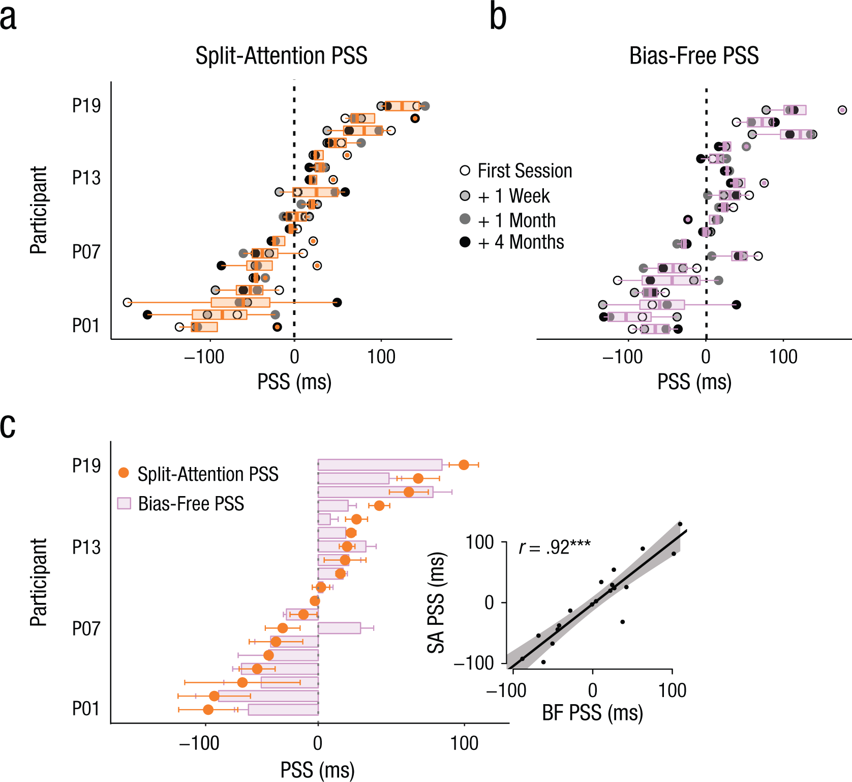
Points of subjective simultaneity (PSSs) for individual participants. The graphs in (a) and (b) show results for the (a) split-attention condition (split-attention PSS) and (b) visual- and auditory-attention conditions combined (bias-free PSS). Each row is for an individual participant. The circles indicate results for the individual sessions, and the box-and-whiskers plots show the within-participant variance across all four sessions. The left and right edges of the boxes represent the first and third quartiles, respectively, and the lines down the center of the boxes represent the medians. The left and right ends of the whiskers represent the minimum and maximum PSSs, respectively. Participants were sorted by the PSS required for the participant to perceive audio and visual stimuli simultaneously, from most negative (i.e., the sound had to be presented first) at the bottom to most positive (i.e., the visual event had to be presented first) at the top. The circles with a different color in the center represent outliers. In (c), both the split-attention PSS and the bias-free PSS are presented for each participant. The results are ordered from the smallest (bottom) to the largest (top) split-attention PSS value. The orange error bars indicate ±1 SEM; the purple error bars indicate +1 SEM. In some cases, the error bars are too small to be seen here. The scatterplot (with best-fitting regression line) in the inset shows the relationship between the split-attention PSS (SA PSS) and the bias-free PSS (BF PSS). The shaded area indicates the 95% confidence interval. The asterisks indicate a significant correlation between the two types of PSS (***p < .001).

Linking the prior-entry effect and PSS

To further investigate the relationship between PSS and the prior-entry effect, we quantified the magnitude of the prior-entry effect by subtracting PSS during visual attention from PSS during auditory attention and tracked its stability over time. The findings suggest that the magnitude of the prior-entry effect was also stable within individuals over the 4-month period, across-session ICC = .46, 95% CI = [.23, .70], F(18, 57) = 4.41, p < .001 (Fig. 3a). Hence, there was a large interindividual variability in the prior-entry effect, but it remained stable over time. In particular, 3 (out of 19) participants showed negative prior-entry effects in at least two of the four sessions; among the remaining participants, six additional prior-entry values were negative. This suggests either that nonattended events were prioritized or that participants did not correctly follow the task instructions. The inclusion or exclusion of these data did not affect the main results of our previous or subsequent analyses, so they were retained.

Fig. 3.

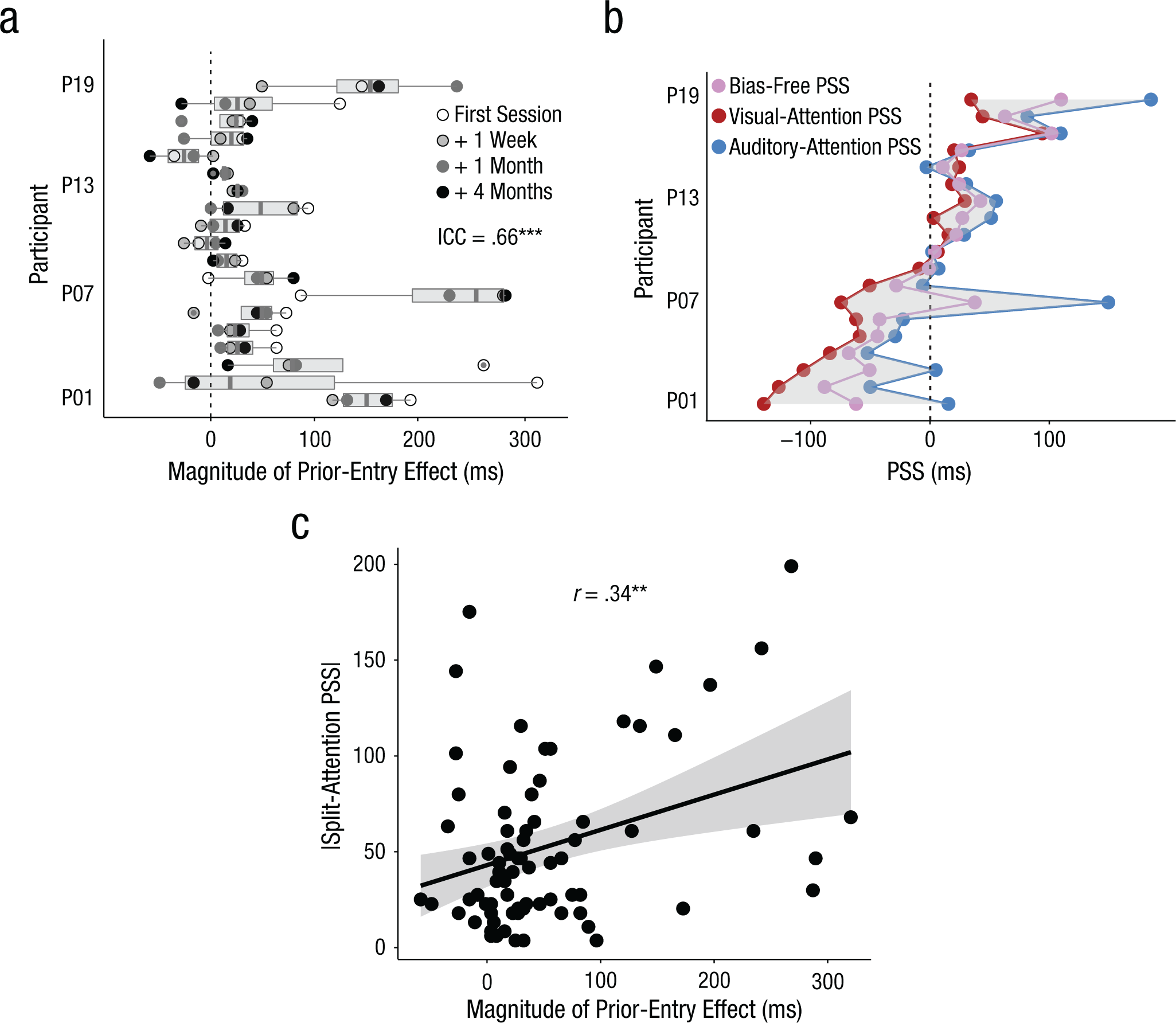
The prior-entry effect for individual participants. The graph in (a) shows the prior-entry effect observed for audiovisual stimuli, computed from visual- and auditory-attention conditions. The circles indicate results for the individual sessions, and the box-and-whiskers plots show the within-participant variance across all four sessions. The left and right edges of the boxes represent the first and third quartiles, respectively, and the lines down the center of the boxes represent the medians. The left and right ends of the whiskers represent the minimum and maximum scores, respectively. The asterisks indicate a significant intraclass correlation coefficient (***p < .001). The graph in (b) shows each participant’s average bias-free, visual-attention, and auditory-attention point of subjective simultaneity (PSS) over the four experimental sessions. The shaded area represents the magnitude of the prior-entry effect. The scatterplot (with best-fitting regression line) in (c) shows the relationship between the absolute value of the PSS in the split-attention condition and the magnitude of the prior-entry effect. Each dot corresponds to an individual at a single session. The shaded area represents the 95% confidence interval. The asterisks indicate a significant correlation (**p < .01).

The extent of the prior-entry effect can be seen as the range of possible values an individual’s PSS took as a function of the individual’s attentional focus (Fig. 3b). Considering that one functional role of prior entry could be compensation for temporal delays to achieve veridical simultaneity (or simultaneity constancy; e.g., Kopinska & Harris, 2004), individuals with a PSS far from veridical simultaneity were predicted to display larger magnitudes of the prior-entry effect. To test this prediction, we calculated the correlation between the magnitude of the prior-entry effect (Fig. 3b, shaded area) and the absolute value of the split-attention PSS values (Fig. 2c) for each individual and for each session. The two were significantly correlated, r = .34, 95% CI = [.13, .53], t(74) = 3.16, p = .002, which suggests that participants with a larger PSS magnitude tended to exhibit larger prior-entry effects (Fig. 3c).

Discussion

In a longitudinal study, we showed the existence of a robust and stable interindividual variability in audiovisual temporal-order perception (and similar variability in auditory and visual temporal-order perception). Our results suggest that temporal order is a psychological bias that is unique to each individual and may result from structural constraints (such as the intrinsic neural delays of a given individual’s brain; Freeman et al., 2013) or from functional constraints akin to hidden-state variables (Wexler, Duyck, & Mamassian, 2015).

Interindividual variability in audiovisual temporal-order perception was observed regardless of whether participants split attention across senses (split-attention PSS) or not (bias-free PSS): The two indices were significantly correlated, which indicates that individual temporal-order bias persisted through manipulation of attention. When participants attended to one or the other sensory modality, shifts in the audiovisual PSS predictably followed the law of prior entry but fluctuated around the individual bias-free PSS. These shifts were consistent over time and opposite in direction to those of the attended sensory modality. We also found that the magnitude of the prior-entry effect was significantly correlated with the absolute value of the split-attention PSS: the further away the individual bias from physical simultaneity, the larger the magnitude of the prior-entry effect. One possible functional interpretation of this finding is that prior entry may reflect brain mechanisms that compensate for individual temporal-order bias or Bayesian priors. In other words, our results suggest that attention mediates the prior-entry effect, enabling an individual’s brain to compensate to some extent for its intrinsic temporal biases.

The existence of a psychological bias in temporal order is consistent with observations that PSSs measured for various stimulus classes (beeps and flashes, audiovisual speech) are correlated within individuals (Love, Petrini, Cheng, & Pollick, 2013) despite differences in integration time (Vatakis & Spence, 2010). Thus, intrinsic biases may depend not on low-level stimulus features but on high-order brain computations, consistent with how temporal-order judgments typically activate parietal cortices (Adhikari, Goshorn, Lamichhane, & Dhamala, 2013; Battelli, Pascual-Leone, & Cavanagh, 2007; Davis, Christie, & Rorden, 2009; Woo, Kim, & Lee, 2009). The extent to which such temporal-order bias plays a role in the integration of information, however, remains unclear: If an individual’s subjective simultaneity has been shown to correlate with the size of the temporal-integration windows in audiovisual speech (Freeman et al., 2013), the PSSs obtained in simultaneity and temporal-order judgment tasks do not correlate (Love et al., 2013; van Eijk et al., 2008). These two measures probably capture different processes, and temporal-integration windows computed across individuals may be confounded by interindividual variability in temporal order. Taken together, these results emphasize the importance of quantifying interindividual differences in psychological and neuroimaging studies (Kanai & Rees, 2011) to shed light on possibly unnoticed neural mechanisms underlying temporal cognition.

Footnotes

Acknowledgements

We thank members of NeuroImagerie Applicative Clinique et Translationnelle for their help in recruiting participants. Preliminary results were presented at the annual meeting of the Association for Psychological Science, in Chicago, May 2016.

Action Editor

Philippe G. Schyns served as action editor for this article.

Declaration of Conflicting Interests

The authors declared that they had no conflicts of interest with respect to their authorship or the publication of this article.

Funding

This work was supported by European Research Council Starting Grant ERC-YStG-263584 (to V. van Wassenhove).

Supplemental Material

Additional supporting information can be found at

Open Practices

All data have been made publicly available via the Open Science Framework and can be accessed at https://osf.io/6n894/. The complete Open Practices Disclosure for this article can be found at http://journals.sagepub.com/doi/suppl/10.1177/0956797616689369. This article has received the badge for Open Data. More information about the Open Practices badges can be found at .

References

Adhikari

B. M.

Goshorn

E. S.

Lamichhane

Dhamala

(2013). Temporal-order judgment of audiovisual events involves network activity between parietal and prefrontal cortices. Brain Connectivity, 3, 536–545. doi:10.1089/brain.2013.0163

Battelli

Pascual-Leone

Cavanagh

(2007). The ‘when’ pathway of the right parietal lobe. Trends in Cognitive Sciences, 11, 204–210. doi:10.1016/j.tics.2007.03.001

Boenke

L. T.

Deliano

Ohl

F. W.

(2009). Stimulus duration influences perceived simultaneity in audiovisual temporal-order judgment. Experimental Brain Research, 198, 233–244. doi:10.1007/s00221-009-1917-z

Colonius

Diederich

(2004). Multisensory interaction in saccadic reaction time: A time-window-of-integration model. Journal of Cognitive Neuroscience, 16, 1000–1009.

Davis

Christie

Rorden

(2009). Temporal order judgments activate temporal parietal junction. Journal of Neuroscience, 29, 3182–3188. doi:10.1523/JNEUROSCI.5793-08.2009

Efron

(1973). Conservation of temporal information by perceptual systems. Perception & Psychophysics, 14, 518–530.

Freeman

E. D.

Ipse

Palmbaha

Paunoiu

Brown

Lambert

. . . Driver

(2013). Sight and sound out of synch: Fragmentation and renormalisation of audiovisual integration and subjective timing. Cortex, 49, 2875–2887. doi:10.1016/j.cortex.2013.03.006

Garner

Lemon

Fellows

Singh

(2012). Irr: Various coefficients of interrater reliability and agreement (Version 0.84) [Software]. Retrieved from https://cran.r-project.org/package=irr

Hallgren

K. A.

(2012). Computing inter-rater reliability for observational data: An overview and tutorial. Tutorial in Quantitative Methods for Psychology, 8(1), 23–34. doi:10.20982/tqmp.08.1.p023

10.

Jaśkowski

(1999). Reaction time and temporal-order judgment as measures of perceptual latency: The problem of dissociations. In Aschersleben

Bachmann

Müsseler

(Eds.), Cognitive contributions to the perception of spatial and temporal events (pp. 265–282). Amsterdam, The Netherlands: North-Holland/Elsevier Science.

11.

Kanai

Rees

(2011). The structural basis of inter-individual differences in human behaviour and cognition. Nature Reviews Neuroscience, 12, 232–242. doi:10.1038/nrn3000

12.

Kopinska

Harris

L. R.

(2004). Simultaneity constancy. Perception, 33, 1049–1060. doi:10.1068/p5169

13.

Kösem

Gramfort

van Wassenhove

(2014). Encoding of event timing in the phase of neural oscillations. NeuroImage, 92, 274–284. doi:10.1016/j.neuroimage.2014.02.010

14.

Love

S. A.

Petrini

Cheng

Pollick

F. E.

(2013). A psychophysical investigation of differences between synchrony and temporal order judgments. PLoS ONE, 8(1), Article e0054798. doi:10.1371/journal.pone.0054798

15.

Noel

J.-P.

Niear

M. D.

Burg

E. V.

Wallace

M. T.

(2016). Audiovisual simultaneity judgment and rapid recalibration throughout the lifespan. PLoS ONE, 11(8), Article e0161698. doi:10.1371/journal.pone.0161698

16.

Rathbone

Shaw

Kumbhare

(2015). ICC.Sample.Size: Calculation of sample size and power for ICC (Version 1.0) [Software]. Retrieved from http://cran.r-project.org/package=ICC.Sample.Size

17.

R Development Core Team. (2016). R: A language and environment for statistical computing (Version 3.2.4) [Computer software]. Retrieved from https://www.r-project.org/index.html

18.

Sanford

E. C.

(1888). Personal equation. American Journal of Psychology, 2, 3–38.

19.

Shore

D. I.

Spence

Klein

R. M.

(2001). Visual prior entry. Psychological Science, 12, 205–212. doi:10.1111/1467-9280.00337

20.

Spence

Parise

(2010). Prior-entry: A review. Consciousness and Cognition, 19, 364–379. doi:10.1016/j.concog.2009.12.001

21.

Spence

Shore

D. I.

Klein

R. M.

(2001). Multisensory prior entry. Journal of Experimental Psychology: General, 130, 799–832.

22.

Spence

Squire

(2003). Multisensory integration: Maintaining the perception of synchrony. Current Biology, 13, R519–R521. doi:10.1016/S0960-9822(03)00445-7

23.

Stone

J. V.

Hunkin

N. M.

Porrill

Wood

Keeler

Beanland

. . . Porter

N. R.

(2001). When is now? Perception of simultaneity. Proceedings of the Royal Society B: Biological Sciences, 268, 31–38. doi:10.1098/rspb.2000.1326

24.

Sugita

Suzuki

(2003). Audiovisual perception: Implicit estimation of sound-arrival time. Nature, 421, 911. doi:10.1038/421911a

25.

Titchener

E. B.

(1908). Lectures on the elementary psychology of feeling and attention. New York, NY: Macmillan.

26.

van Eijk

R. L.

Kohlrausch

Juola

J. F.

van de Par

(2008). Audiovisual synchrony and temporal order judgments: Effects of experimental method and stimulus type. Perception & Psychophysics, 70, 955–968. doi:10.3758/PP.70.6.955

27.

van Wassenhove

Grant

K. W.

Poeppel

(2007). Temporal window of integration in auditory-visual speech perception. Neuropsychologia, 45, 598–607. doi:10.1016/j.neuropsychologia.2006.01.001

28.

Vatakis

Spence

(2010). Audiovisual temporal integration for complex speech, object-action, animal call, and musical stimuli. In Naumer

M. J.

Kaiser

(Eds.), Multisensory object perception in the primate brain (pp. 95–121). New York, NY: Springer.

29.

Vroomen

Keetels

de Gelder

Bertelson

(2004). Recalibration of temporal order perception by exposure to audio-visual asynchrony. Cognitive Brain Research, 22, 32–35. doi:10.1016/j.cogbrainres.2004.07.003

30.

Weiss

Hilkenmeier

Scharlau

(2013). Attention and the speed of information processing: Posterior entry for unattended stimuli instead of prior entry for attended stimuli. PLoS ONE, 8(1), Article e0054257. doi:10.1371/journal.pone.0054257

31.

Wexler

Duyck

Mamassian

(2015). Persistent states in vision break universality and time invariance. Proceedings of the National Academy of Sciences, USA, 112, 14990–14995. doi:10.1073/pnas.1508847112

32.

Woo

S.-H.

Kim

K.-H.

Lee

K.-M.

(2009). The role of the right posterior parietal cortex in temporal order judgment. Brain and Cognition, 69, 337–343. doi:10.1016/j.bandc.2008.08.006

33.

World Medical Association. (2013). WMA Declaration of Helsinki: Ethical principles for medical research involving human subjects. Retrieved from http://www.wma.net/en/30publications/10policies/b3/

34.

Zampini

Shore

D. I.

Spence

(2003). Audiovisual temporal order judgments. Experimental Brain Research, 152, 198–210. doi:10.1007/s00221-003-1536-z

Supplementary Material

Please find the following supplemental material available below.

For Open Access articles published under a Creative Commons License, all supplemental material carries the same license as the article it is associated with.

For non-Open Access articles published, all supplemental material carries a non-exclusive license, and permission requests for re-use of supplemental material or any part of supplemental material shall be sent directly to the copyright owner as specified in the copyright notice associated with the article.

0.00 MB

0.38 MB