
Abstract
When staring at a blank grid, one can readily “see” simple shapes—a peculiar experience that does not occur when viewing an empty background. But just what does this “seeing” entail? Previous work has explored many cues to object-based attention (e.g., involving continuity and closure), but here we asked whether attention can be object based even when there are no cues to objecthood. Observers viewed simple grids and attended to particular squares until they could effectively “see” shapes such as a capital H or I. During this scaffolded attention, two probes appeared, and observers reported whether they were the same or different. Remarkably, this produced a traditional same-object advantage: In several experiments (including high-powered direct replications), performance was enhanced for probes presented on the same (purely imagined) object, compared with equidistant probes presented on different objects. We conclude that attention not only operates over objects but also can effectively create object representations.
A curious thing can happen when you stare at a gridlike pattern, as in graph paper, tiles on a bathroom floor, or the grid in Figure 1a. Although such patterns contain no structure, you may often “see” structure anyway; for example, while staring at Figure 1a, you may find yourself momentarily seeing a block-letter H (Fig. 1b). This phenomenon appears to be based on attention to relevant squares of the grid, and these squares do indeed accrue attentional benefits, such as faster probe detection (Podgorny & Shepard, 1978, 1983). We will call this phenomenon scaffolded attention because of how the grid provides a scaffold for selection. (Note that you cannot see these same shapes when staring at a blank page.) Whereas past work focused on the attended squares, the present study focused (for the first time, to our knowledge) on the shapes themselves. We asked whether this form of attention ends up creating bona fide object representations that then enjoy object-specific effects.
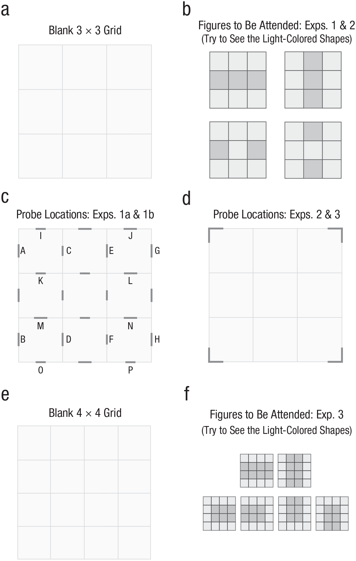
Sample grids, patterns, and probes. While staring at the blank 3 × 3 grid (a), readers may come to see simple shapes, such as a block-letter H or a block-letter I. This grid is of the sort used in Experiments 1a, 1b, 2a, and 2b. The subsequent panels show (b) the different figures that observers were asked to imagine while staring at a blank grid in Experiments 1a, 1b, 2a, and 2b; (c) the line probes used in Experiments 1a and 1b (with labels included here for easier reference to the main text); (d) the corner probes used in Experiments 2a and 2b; (e) a blank 4 × 4 grid of the sort used in Experiments 3a and 3b; and (f) the different figures that observers were asked to imagine in Experiments 3a and 3b.
A central question for any process concerns the units over which it operates. Whereas visual attention was traditionally thought to select spatial regions (as in a spotlight; see Cave & Bichot, 1999), later work demonstrated that attention often selects only discrete objects (see Scholl, 2001). This object-based attention has been supported by many studies, from selective looking (e.g., Neisser & Becklen, 1975) to multiple-object tracking (e.g., Pylyshyn & Storm, 1988) to unilateral neglect (e.g., Tipper & Behrmann, 1996). The most well-studied form of evidence for object-based attention, however, is the same-object advantage: Selecting (or shifting between) two visual features is easier when they are on the same object, compared with equidistant points on different objects (e.g., Duncan, 1984; Egly, Driver, & Rafal, 1994).
But what counts as an object? The answer may often seem obvious (as in experiments with two rectangular bars in different locations; e.g., Egly et al., 1994), and past studies have identified roles for particular cues such as closure (Marino & Scholl, 2005) and continuity (Feldman, 2007). Here, in contrast, we asked whether object-based attention can also operate over “objects” that are not defined by any explicit cues and, in particular, whether the shapes created by scaffolded attention give rise to same-object advantages. If they do, this would indicate an unexpected inversion of the typical relationship between objects and attention, showing the existence of not only object-based attention but also attention-based objects.
Experiment 1a: Probed Lines on Imagined Objects
Observers attended to 3 × 3 grids to “see” various shapes (e.g., a block-letter H). Two lines from Figure 1c then flashed, and observers reported whether they were the same length.
Method
Observers
Ten observers from the Yale and New Haven communities participated in exchange for monetary payment. Four observers were excluded and replaced before any analyses were conducted because they reported (during subsequent debriefing questions) that they had not imagined the shapes for the entire duration, as instructed below. This sample size was determined before data collection began (arbitrarily rounded up from the sample sizes of 6 to 8 that were used in the only previous studies of what we are calling scaffolded attention; Podgorny & Shepard, 1978, 1983), and it gave us 89% power to detect a same-object advantage of the average effect size of the seven experiments reported here. This sample size was then fixed to be identical across five of the seven experiments reported here (including two direct replications), with the other two experiments (also direct replications) having quadrupled sample sizes.
Apparatus
Stimuli were presented using custom software written in Python with the PsychoPy libraries (Peirce et al., 2019) and were displayed on a monitor with a 60-Hz refresh rate. Observers sat in a dimly lit room without restraint approximately 60 cm from the display (with all visual extents reported below based on this approximate viewing distance). The functional part of the display subtended 34.87° × 28.21°.
Stimuli
Observers viewed three display elements on each trial: a grid of squares, an instruction prompt, and a countdown timer. Each display included a 3 × 3 grid of light gray (RGB values = 245, 245, 245) squares (each subtending 3°) bounded by 0.03° lines (RGB values = 203, 203, 203), presented at the center of the display on a white background. Centered on each side of each square was a darker (RGB values = 128, 128, 128) potential-probe line (0.08°), the length of which was randomly set on each trial to be either short (0.72°) or long (0.90°), with the exception of the two actively probed lines on each trial, as described below. The two lines that were actively probed on each trial were highlighted by turning them green (RGB values = 0, 201, 0). The probes in each potential pair were constrained to have their centers exactly 6° apart, thus yielding (as depicted in Fig. 1c) four potential vertical-probe pairs (AB, CD, EF, GH) and four potential horizontal-probe pairs (IJ, KL, MN, OP). (Each display included all potential-probe lines so that the actual probes, when they occurred, were better integrated into the imagined objects.)
An instruction prompt was also presented on each trial, centered 8° above the center of the display, with its text drawn in a black Monaco font, sized so that the maximum character height was 0.4°. This prompt always consisted of the word “Imagine,” followed by one of four symbols— ,
,  ,
,  , or
, or  —corresponding to the four shapes depicted in Figure 1b. A countdown timer (with its digits drawn in the same font size) was also presented on each trial, centered 5.5° above the center of the display. This timer began with the single digit “5,” which was replaced each second with the next lowest integer until it disappeared (1 s after the appearance of the digit “1”).
Procedure
Each trial began with the presentation of the grid, the instruction prompt, and the timer. During the timer’s countdown, observers were to attend to the squares indicated by the instruction prompt, and they had to imagine the relevant figure “until you can ‘see’ [it] superimposed on the grid.” Two of the potential probe lines then turned green for 250 ms immediately after the countdown timer disappeared, after which the entire display disappeared, being replaced by the response prompt “Same or different?” (drawn in the same font as the instruction prompt), presented in the center of the display. The two lines probed on each trial were equally often the same length (either long-long or short-short) or different lengths (short-long); these possibilities occurred equally often in each condition type as described below. Observers pressed one of two keys to indicate their response, after which there was a blank delay for 500 ms before the next trial began.
Design
Each of the eight possible probe pairs (four vertical, four horizontal) as listed in Figure 1c was tested equally often with each of the four instruction prompts (, , , ), but whether these pairs were categorized as same-object or different-object probe pairs depended on the specific prompt. When observers were prompted to imagine two vertical lines (i.e., , corresponding to the upper-right panel in Fig. 1b), the same-object pairs were AB, CD, EF, and GH, and the different-object pairs were IJ, KL, MN, and OP. In contrast, when observers were prompted to imagine two horizontal lines (i.e., , corresponding to the upper-left panel in Fig. 1b), the same-object pairs were IJ, KL, MN, and OP, and the different-object pairs were AB, CD, EF, and GH. Both of these stimuli were chosen to clearly indicate multiple objects in the same kind of two-rectangles configuration that has so often been used to demonstrate same-object advantages (Egly et al., 1994). These same pairs were also contrasted in the two control shapes ( and , as in the bottom two panels in Fig. 1b), where observers also attended to the central square, which effectively connected the parallel lines into single objects (using physical connectedness, which is perhaps the most powerful cue to grouping and object formation; Wagemans, Elder, et al., 2012).
There were thus 64 different trial types: 4 imagined (i.e., attended) shapes (, , , or , as depicted in Fig. 1b) × 8 potential-probe pairs (AB, CD, EF, GH, IJ, KL, MN, OP, as depicted in Fig. 1c) × 2 correct responses (same vs. different). Observers completed one block of 64 practice trials (1 of each type, presented in a different random order for each observer), the results of which were not recorded. They then completed two experimental blocks of 64 trials (1 of each type per block, presented in a different random order for each observer). A written prompt encouraged them to take a short self-timed break between the two blocks. Finally, observers completed a debriefing procedure, during which they were asked about how they had used the 5 s allotted for them to attend to the squares and about any other strategies they might have used.
Results
The two conditions with multiple imagined objects ( and ) yielded a same-object advantage (as depicted in Fig. S1a in the Supplemental Material available online): Performance (reporting same probe lengths vs. different probe lengths) was better for same-object probe pairs than for different-object probe pairs (60.63% vs. 53.44%), t(9) = 3.02, p = .014, d = 0.96, 95% confidence interval (CI) for Cohen’s d = [0.18, 1.70], with all but 2 of the observers showing numerical effects in this direction. In contrast, no such effect emerged when these same probe pairs were contrasted while observers were imagining the two control shapes ( and ; 55.94% vs. 60.31%), t(9) = 1.50, p = .168, d = 0.47, 95% CI = [–0.19, 1.12], with the interaction (i.e., the difference of differences) between these two comparisons also being highly reliable, t(9) = 3.32, p = .009, d = 1.05, 95% CI = [0.25, 1.81].
For completeness, we can also break these effects down by orientation, although these comparisons can never influence our primary questions or analyses, which always averaged across equal numbers of configurations in each orientation. The same-object advantage was reliable when we compared only horizontal rectangles, t(9) = 3.33, p = .009, d = 1.05, 95% CI = [0.25, 1.82], but not when we compared only vertical rectangles, t(9) = 0.64, p = .537, d = 0.20, 95% CI = [–0.43, 0.82].
Experiment 1b: Direct Replication
Method
This experiment was a direct replication of Experiment 1a. Ten new observers participated (with this sample size chosen to exactly match that of Experiment 1a). Five additional observers were excluded and replaced before any analyses (using the same exclusion criteria as in Experiment 1a).
Results
The pattern of results in this direct replication (depicted in Fig. S1b in the Supplemental Material) exactly mirrored that of Experiment 1a: There was a reliable advantage for same-object probe pairs compared with different-object probe pairs for the two conditions with multiple imagined objects (61.25% vs. 53.13%), t(9) = 3.28, p = .009, d = 1.04, 95% CI = [0.24, 1.80] (with all but 2 observers showing this trend), but not for the control shapes (59.69% vs. 61.25%), t(9) = 0.47, p = .647, d = 0.15, 95% CI = [–0.48, 0.77], along with a reliable interaction, t(9) = 2.43, p = .038, d = 0.77, 95% CI = [0.04, 1.46]. The same-object advantage was only marginal, however, when we limited the data to only horizontal rectangles, t(9) = 2.08, p = .068, d = 0.66, 95% CI = [–0.05, 1.33], or vertical rectangles, t(9) = 1.95, p = .082, d = 0.62, 95% CI = [–0.08, 1.28].
Experiment 2a: Probed Corners on Imagined Objects
In Experiments 1a and 1b, same-object (but not different-object) probed lines were always parallel to their imagined objects. To ensure that this phenomenon did not merely reflect such congruent parallelism, we tested for same-object advantages using corner probes (Fig. 1d).
Method
This experiment was identical to Experiments 1a and 1b, except where noted. Ten observers participated for monetary payment or class credit (with this preregistered sample size chosen to exactly match that of Experiments 1a and 1b). Only one observer was excluded (via the same criteria discussed above) and replaced before any analyses were conducted.
There were four possible probe pairs, corresponding to the top two corners, the bottom two corners, the left two corners, or the right two corners of the 3 × 3 grid. The segments of the probe corners were the same color and thickness as the probe lines from Experiments 1a and 1b and were either both short (0.72°) or both long (0.90°), intersecting at the corner points as depicted in Figure 1d.
Each of the four possible probe pairs was tested equally often with each of the four instruction prompts (, , , or ), but whether these pairs were categorized as same-object or different-object probe pairs again depended on the specific prompt. When observers were prompted to imagine two vertical lines (i.e., , corresponding to the upper-right panel in Fig. 1b), the same-object pairs were the left two corners and the right two corners, and the different-object pairs were the top two corners and the bottom two corners. In contrast, when observers were prompted to imagine two horizontal lines (i.e., , corresponding to the upper-left panel in Fig. 1b), the same-object pairs were the top two corners and the bottom two corners, and the different-object pairs were the left two corners and the right two corners. These same pairs were also contrasted in the two control shapes ( and , as in the bottom two panels in Fig. 1b), where observers also attended to the central square, which effectively connected the parallel lines into single objects.
In Experiments 1a and 1b, the probes appeared via a color change, with the potential-probe lines themselves having been explicitly highlighted (in gray) during the initial scaffolded-attention phase. In contrast, the corner probes in the current experiment were never previewed in this manner; instead, they appeared all at once (still in green) after the scaffolded-attention phase of each trial was complete. (We made this change because some observers from the previous experiments admitted that during the scaffolded-attention phase, they sometimes explored the potential-probe lines rather than trying to see the relevant shapes. That temptation might have been even greater in the present experiment because there were only 4 potential probe locations rather than 24, but it was removed in the present experiment by effectively eliminating the potential probes altogether.) Observers reported whether the sizes of the two corner probes were the same (i.e., long-long or short-short) or different (i.e., short-long).
There were 32 different trial types: 4 imagined or attended shapes (, , , or , as depicted in Fig. 1b) × 4 potential-probe pairs (top two corners, bottom two corners, left two corners, right two corners, as depicted in Fig. 1d) × 2 correct responses (same vs. different). Observers completed one block of 32 practice trials (1 of each type, presented in a different random order for each observer), the results of which were not recorded. In each of two experimental blocks, each observer completed two repetitions for each of the 32 trial types, for a total of 64 trials (presented in a random order for each observer).
Results
The pattern of results (depicted in Fig. S2a in the Supplemental Material) exactly mirrored that of Experiments 1a and 1b: There was a reliable advantage for same-object probe pairs compared with different-object probe pairs for the two conditions with multiple imagined objects (66.88% vs. 55.93%), t(9) = 4.87, p < .001, d = 1.54, 95% CI = [0.59, 2.46] (with all but 1 observer showing this trend), but not for the control shapes (66.25% vs. 63.75%), t(9) = 0.85, p = .417, d = 0.27, 95% CI = [–0.37, 0.89], along with a reliable interaction, t(9) = 2.36, p = .043, d = 0.75, 95% CI = [0.02, 1.44]. The same-object advantage was also reliable when we considered only horizontal rectangles, t(9) = 2.85, p = .019, d = 0.90, 95% CI = [0.14, 1.63], or vertical rectangles, t(9) = 2.29, p = .048, d = 0.72, 95% CI = [0.01, 1.41].
Experiments 2b and 2c: Direct Replications
Method
These experiments were direct replications of Experiment 2a. Ten new observers participated in Experiment 2b (with this preregistered sample size chosen to exactly match that of Experiments 1a, 1b, and 2a), and 40 new observers participated in Experiment 2c (with this preregistered sample size giving us an increased power of > 99% to detect a same-object advantage of the average effect size of the seven experiments reported here). No observers were excluded in either experiment.
Results
The patterns of results in these direct replications exactly mirrored those of Experiment 2a. The results of the higher powered replication (Experiment 2c) are depicted in Figure 2a, and the results of the initial replication (Experiment 2b) are depicted in Figure S2b in the Supplemental Material. There was a reliable advantage for same-object probe pairs compared with different-object probe pairs for the two conditions with multiple imagined objects—Experiment 2b: 60.94% vs. 53.44%, t(9) = 2.48, p = .035, d = 0.78, 95% CI = [0.05, 1.48]; Experiment 2c: 60.55% vs. 53.91%, t(39) = 5.20, p < .001, d = 0.82, 95% CI = [0.46, 1.18]—but not for the control shapes—Experiment 2b: 54.69% vs. 57.19%, t(9) = 0.85, p = .417, d = 0.27, 95% CI = [–0.37, 0.89]; Experiment 2c: 60.16% vs. 59.92%, t(39) = 0.11, p = .916, d = 0.02, 95% CI = [–0.29, 0.33]. There was also a highly reliable interaction—Experiment 2b: t(9) = 3.93, p = .003, d = 1.24, 95% CI = [0.39, 2.06]; Experiment 2c: t(39) = 2.40, p = .021, d = 0.38, 95% CI = [0.06, 0.70]. In both experiments, the same-object advantage was reliable when we compared only horizontal rectangles—Experiment 2b: t(9) = 2.85, p = .019, d = 0.90, 95% CI = [0.14, 1.63]; Experiment 2c: t(39) = 4.47, p < .001, d = 0.71, 95% CI = [0.36, 1.05]—but not when we compared only vertical rectangles—Experiment 2b: t(9) = 0.87, p = .405, d = 0.28, 95% CI = [–0.36, 0.90]; Experiment 2c: t(39) = 1.67, p = .103, d = 0.26, 95% CI = [–0.05, 0.58].

Results from (a) Experiment 2c and (b) Experiment 3b, both employing corner probes in high-powered replications. The left panels depict the mean accuracy in each condition (unconnected objects, connected objects) of reporting whether the two corner probes had segments of the same or different lengths. Error bars reflect 95% confidence intervals after the shared variance was subtracted, and the dashed lines represent chance performance. The right panels depict the nonparametric results (ordered by effect magnitude) for the key same-object advantage in the unconnected-objects condition. In these panels, green bars represent observers who had same-object advantages for the unconnected-objects condition, and the red bars represent observers who had the opposite pattern for that condition.
Experiments 3a and 3b: Larger Grids
In the previous experiments, connected objects involved seven squares, whereas unconnected objects involved six squares. To ensure that the results did not simply reflect a limit (of 6) on the number of attendable squares, we had observers imagine objects on a larger (4 × 4) grid (Figs. 1e and 1f).
Method
These experiments were identical to Experiments 2a, 2b, and 2c, except as noted. Ten new observers participated in Experiment 3a (with this preregistered sample size chosen to exactly match that of Experiments 1a, 1b, 2a, and 2b), and 40 new observers participated in Experiment 3b (with this preregistered sample size chosen to exactly match that of Experiment 2c). Three additional observers (1 in Experiment 3a, 2 in Experiment 3b) were excluded and replaced before any analyses were conducted (using the same exclusion criteria as in the previous experiments).
Each display now included a 4 × 4 grid (of the same squares used in the previous experiments), and observers were asked to imagine one of six shapes (as depicted in Fig. 1f:  ,
,  ,
,  ,
,  , or ). Unconnected objects (, ) now involved 8 squares, and connected objects (, , , ) involved 10 squares. The same four potential-probe pairs (now with “long” lengths of 0.98°) were tested, corresponding to the top two corners, the bottom two corners, the left two corners, or the right two corners of the 4 × 4 grid (Fig. 1d). Each of the four possible probe pairs was tested equally often with each of the six attended shapes.
There were 48 trial types: 6 attended shapes (, , , , , or , as depicted in Fig. 1f) × 4 potential-probe pairs (top two corners, bottom two corners, left two corners, right two corners, as depicted in Fig. 1d) × 2 correct responses (same vs. different). Observers completed one block of 48 practice trials (1 of each type, presented in a different random order for each observer), the results of which were not recorded. In each of two experimental blocks, each observer completed each of the 48 trial types (presented in a random order for each observer).
Results
The patterns of results in these experiments exactly mirrored those of all the previous experiments. The results of the higher powered replication (Experiment 3b) are depicted in Figure 2b, and the results of the initial experiment (Experiment 3a) are depicted in Figure S3 in the Supplemental Material. There was a reliable advantage for same-object probe pairs compared with different-object probe pairs for the two conditions with multiple imagined objects—Experiment 3a: 65.00% vs. 48.75%, t(9) = 3.03, p = .014, d = 0.96, 95% CI = [0.18, 1.70]; Experiment 3b: 63.91% vs. 51.88%, t(39) = 5.00, p < .001, d = 0.79, 95% CI = [0.43, 1.14]—but not for the control shapes—Experiment 3a: 57.81% vs. 59.69%, t(9) = 0.58, p = .576, d = 0.18, 95% CI = [–0.45, 0.80]; Experiment 3b: 57.89% vs. 59.06%, t(39) = 0.79, p = .432, d = 0.13, 95% CI = [–0.19, 0.44]. There was also a reliable interaction—Experiment 3a: t(9) = 2.29, p = .048, d = 0.73, 95% CI = [0.01, 1.41]; Experiment 3b: t(39) = 4.63, p < .001, d = 0.73, 95% CI = [0.38, 1.08]. In both experiments, the same-object advantage was reliable when we compared only horizontal rectangles—Experiment 3a: t(9) = 3.21, p = .011, d = 1.01, 95% CI = [–0.35, 0.92]; Experiment 3b: t(39) = 4.99, p < .001, d = 0.79, 95% CI = [0.27, 0.95]—but not when we compared only vertical rectangles—Experiment 3a: t(9) = 1.94, p = .085, d = 0.61, 95% CI = [–0.08, 1.28]; Experiment 3b: t(39) = 1.86, p = .071, d = 0.29, 95% CI = [–0.03, 0.61].
General Discussion
The phenomenon reported here was inspired by the peculiar yet commonplace experience that when staring at a blank grid, one can readily “see” simple shapes—something that does not occur when viewing an empty background. Inspired by the only two previous studies of this phenomenon of which we are aware (Podgorny & Shepard, 1978, 1983), we termed this scaffolded attention and hypothesized that this odd experience results from attention effectively forming object representations (perhaps even making them appear shaded, as in Figs. 1b and 1f; Tse, 2005). The experiments here support this possibility by demonstrating same-object advantages in objective performance: Observers were better at comparing two probes when they were on the same (purely imagined) object.
We speculate that this phenomenon may reflect the intimate relationship between attention and perceptual grouping (see Wagemans, Feldman, et al., 2012). Researchers have occasionally noted that this relationship may be bidirectional: Beyond attention driven by grouping cues, “you can also modulate subjective grouping at will to some extent in many grouping displays, especially when the stimulus factors are relatively subtle” (Driver, Davis, Russell, Turatto, & Freeman, 2001, p. 90). The grids employed here may constitute the subtlest possible “stimulus factors,” providing the raw material (i.e., the squares) that can be grouped without any overt image cues to compete with voluntary attention. Thus, attention to the relevant squares effectively groups them, forming object representations out of thin (scaffolded) air.
Supplemental Material
Ongchoco-Scholl_Supplemental_Material_rev – Supplemental material for How to Create Objects With Your Mind: From Object-Based Attention to Attention-Based Objects
Supplemental material, Ongchoco-Scholl_Supplemental_Material_rev for How to Create Objects With Your Mind: From Object-Based Attention to Attention-Based Objects by Joan Danielle K. Ongchoco and Brian J. Scholl in Psychological Science
Footnotes
Acknowledgements
We thank Jay Pratt and the members of the Yale Perception and Cognition Laboratory for helpful comments.
Action Editor
Alice J. O’Toole served as action editor for this article.
Author Contributions
Both authors designed the research and wrote the manuscript. J. D. K. Ongchoco conducted the experiments and analyzed the data with input from B. J. Scholl. Both authors approved the final manuscript for submission.
Declaration of Conflicting Interests
The author(s) declared that there were no conflicts of interest with respect to the authorship or the publication of this article.
Funding
This project was funded by the Office of Naval Research Multidisciplinary University Research Initiative Grant No. N00014-16-1-2007 awarded to B. J. Scholl.
Open Practices
The raw data for these experiments can be viewed in the Supplemental Material available online, and the preregistrations for each experiment can be accessed at http://aspredicted.org/blind.php?x=um27pp (Experiments 2a and 2b), http://aspredicted.org/blind.php?x=j9xe2s (Experiment 2c), and ![]() (Experiment 3b).
(Experiment 3b).
References
Supplementary Material
Please find the following supplemental material available below.
For Open Access articles published under a Creative Commons License, all supplemental material carries the same license as the article it is associated with.
For non-Open Access articles published, all supplemental material carries a non-exclusive license, and permission requests for re-use of supplemental material or any part of supplemental material shall be sent directly to the copyright owner as specified in the copyright notice associated with the article.