Perceptual Awareness Occurs Along a Graded Continuum: No Evidence of All-or-None Failures in Continuous Reproduction Tasks

Abstract

Does sensory information reach conscious awareness in a discrete, all-or-nothing manner or a gradual, continuous manner? To answer this question, we examined behavioral performance across four different paradigms that manipulate visual awareness: the attentional blink, backward masking, the Sperling iconic memory paradigm, and retro-cuing. We then asked how well we could account for participants’ (N = 112 adults) behavior using a signal detection framework that factors in psychophysical scaling to model participants’ responses along a single continuum. We found that this model easily accounted for the data from each of these diverse paradigms. Moreover, we reanalyzed the data from prior studies that had posited a discrete view of perceptual awareness and found that our continuous signal detection model outperformed the models that had been used to support an all-or-nothing view of consciousness. This set of data is consistent with the idea that conscious awareness occurs along a graded continuum.

Keywords

attention awareness consciousness perception signal detection theory vision

How does information transition from being unconsciously processed to being accessed by conscious awareness? According to some models, information reaches awareness in a graded fashion that varies along a continuum associated with the intensity of the stimulus, attention, or cortical activity (Elliott et al., 2016; Nieuwenhuis & de Kleijn, 2011; Overgaard et al., 2006; Phillips, 2020). Under this view, there is a continuous transition from unconscious to conscious processing leading to varying levels of vague or unclear perceptual experiences. According to other models, information reaches awareness in a discrete manner associated with all-or-nothing changes in neural activity (Carruthers, 2019; Dehaene et al., 2001; Lamme, 2003; Sergent & Dehaene, 2004; Vul et al., 2009). In this case, the transition from unconscious to conscious is binary; participants either do or do not perceive a particular stimulus.

Over the past few decades, researchers on both sides of this debate have used numerous experimental paradigms (e.g., the attentional blink, visual masking) and methodologies (e.g., objective measurements, subjective ratings) to assess this question, often making it difficult to compare studies with one another. Recently, however, one tool that has been applied to this debate is probabilistic mixture modeling. This particular modeling framework takes participants’ responses in a continuous reproduction task (e.g., what color was this stimulus on a color wheel?) and models the errors that participants make on this task (Bays et al., 2009; Zhang & Luck, 2008). Although it was initially proposed to model visual working memory, mixture modeling has since been applied to nearly all areas of perception, attention, and long-term memory research (Brady et al., 2013; Golomb et al., 2014; Salahub & Emrich, 2016). In its simplest form, the mixture model framework posits that the representation of a stimulus often fails completely (i.e., it is not encoded/remembered, resulting in guesses) and that when it does not fail completely, its representation varies in precision, which can be quantified. These two states are often modeled by a combination of a von Mises distribution and a uniform distribution to quantify the precision of represented items and the rates of not having a representation of an item. Because this modeling approach differentiates between instances in which items are and are not successfully represented in both a continuous (i.e., precision) and a discrete (i.e., guess rate) manner, it is a natural tool for asking whether information transitions into conscious awareness in a discrete or graded manner.

One example of this approach is the nature of perceptual awareness in the attentional blink (Raymond et al., 1992). The attentional blink is a perceptual phenomenon in which participants less accurately perceive the second of two targets when it appears close in time to the first target. By asking participants to report the identity of the second target in a continuous manner (e.g., on a color wheel), we can model the precision and guess rates of the second target, assessing whether the second item sometimes goes unnoticed (i.e., guess rate increases) or is always perceived but less precisely (i.e., precision degrades). Using this approach, Asplund et al. (2014) found that the guess rate of the second target increased while the precision of those responses stayed the same. In other words, information reached conscious awareness in a quantal, all-or-nothing manner (but see Sy et al., 2021). Similar work has been done in many other paradigms, including the Sperling iconic memory paradigm (Pratte, 2018) and a related retro-cuing paradigm (Thibault et al., 2016), with each case supporting some form of discrete failures of consciousness on the basis of mixture model fits.

Recently, however, theoretical work by Schurgin et al. (2020) has undermined foundational assumptions of mixture models and shown that in the case of visual working memory and visual long-term memory, this modeling approach does not reveal two distinct psychological processes. Specifically, Schurgin et al. showed that precision and guess rate do not change independently of one another; instead, they always change together, as though they are really just different reflections of a single underlying construct. Schurgin et al. showed how a simple model with only a single latent variable—what they call memory strength—can account for data that were thought to require a mixture of guesses and precision errors. The reason this was not previously recognized is that standard mixture models do not consider the psychophysical similarity of items, which is deeply nonlinear. For example, colors that are 5° apart on the color wheel appear more similar to one another than colors that are 35° apart. However, colors that are 120° apart do not appear more similar than colors that are 150° apart. By considering the psychophysical similarity of items in a given stimulus space, Schurgin et al. showed that performance on working memory and long-term memory tasks could be explained by a signal detection framework in which a continuous representational strength (d′) is the only varying parameter. This work forms the basis of the target confusability competition (TCC) model, which posits that all stimuli in a memory or perception task are processed with varying degrees of noise, leading to reproduction errors.

Statement of Relevance

At any given moment, the human senses (e.g., vision, hearing) are presented with more information than the brain can process. Some of this information ultimately reaches conscious awareness (e.g., the sight of an animal crossing the road in front of you), whereas other information remains unconscious (e.g., the pothole on the street that you drive right over because you failed to notice it). How does information transition from unconscious to conscious? Does it enter in an abrupt, all-or-nothing manner? Or does it enter along a graded continuum? Here, we used a wide array of paradigms that manipulate perceptual awareness and found that a signal detection-based model, which posits that information reaches consciousness in a graded fashion, easily explains all of these results. Moreover, this model outperformed other models that have been cited to claim that information reaches consciousness in a discrete fashion. Thus, we argue that information reaches consciousness along a graded continuum.

In the current work, we asked how well this continuous TCC model fits the data from four different paradigms that manipulate visual awareness: the attentional blink, backward masking, the Sperling paradigm, and retro-cuing. For three of these paradigms, we reanalyzed data from prior studies claiming to show discrete failures of conscious awareness. In each of these cases, however, formal model comparisons show that the continuous TCC model outperforms mixture models, which suggests that information reaches conscious awareness in a continuous, graded manner.

Method

The TCC model

In a standard working memory experiment, participants were asked to remember a small number of items (e.g., five colors) and respond in a continuous space (e.g., a color wheel; Fig. 1a). The resulting data from these experiments are a distribution centered around zero with long, fat tails with many errors far from zero. Under the mixture modeling framework proposed by Zhang and Luck (2008) and since elaborated (e.g., Bays et al., 2009; Pratte, 2018), this distribution is thought to comprise two components related to (a) the precision of items successfully processed and reported (i.e., the standard deviation) and (b) how frequently items fail to be processed and are not represented (i.e., the guess rate). Recent work has strongly questioned this idea that there are two distinct factors underlying performance in continuous reproduction tasks, however (e.g., Bays, 2014; Schurgin et al., 2020; van den Berg et al., 2012). In the TCC framework of Schurgin et al. (2020), for example, this response distribution is thought of as a relatively simple outcome of noise being added to perceptual signals. In particular, TCC proposes that psychophysical similarity (i.e., measuring how perceptually confusable each item is with the item to be remembered; target confusability) and signal detection theory (i.e., noisy decision making, a kind of competition; MacMillan & Creelman, 1991) account for performance. Critically, according to the TCC model, there is no distinction between how precisely and how many items are processed—only a single latent variable, the strength of the item’s representation, is needed to account for performance in continuous reproduction (Schurgin et al., 2020). Thus, if the TCC model accurately fits data from tasks in which perception is challenging, this would suggest that conscious perception can potentially be thought of as a graded phenomenon with the strength of a given percept varying along a single continuum.

Fig. 1.

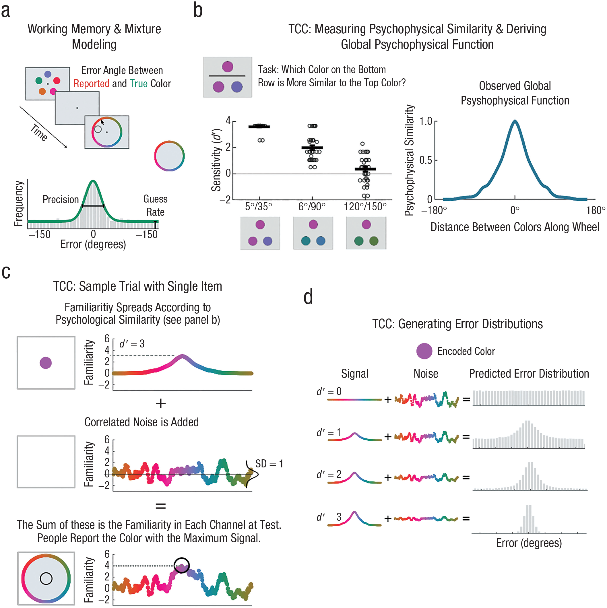
The target confusability competition (TCC) model. (a) Continuous report working memory task. Participants are shown a stimulus display, and after a delay, they are asked to report the exact color of a cued item with the color wheel. In the lower panel is an example of a mixture model’s fit to continuous report data. Most results land within a small range centered around the target’s true color, with some responses being far off. The standard mixture model (Zhang & Luck, 2008) approach states that these responses can be successfully modeled by assuming that errors occur because an observer either remembers nothing about the item (guesses) or has a noisy representation of that item (precision). (b) To measure the psychophysical similarity function of a stimulus space, we had participants perform a triad similarity task and report which of two colors (bottom left) was more similar to the target (top left). Although the difference between the two colors was always exactly the same (30°), d′ decreased as the choices were further from the target. From this, we can plot the global psychophysical function for all colors using this triad task (right). The key point here is that this similarity function is not linear and is approximately exponential when perceptual noise is properly considered. (c) This model can be visualized with a single trial. When an observer encodes the color purple with a strength (d′) of 3, the familiarity of purple, as well as nearby/similar colors, is increased relative to the psychophysical similarity function (b). Then, after adding noise to every color channel, observers make decisions on the basis of which color has the maximum signal. (d) Predicted error distributions can be generated simply as a function of varying d′ and combining it with correlated noise. Thus, for any observed error distribution, d′ is simply altered until the best fit to the data is found.

To intuitively understand the TCC model, one may consider a situation in which an observer is shown a colored item and is asked to report the color of that item in a continuous report task with a color wheel. It is natural to assume that every color around the color wheel would get varying degrees of a “familiarity boost” depending on the similarity between the target color and the response colors. For example, when the presented color is a shade of purple, this color gets a big boost in familiarity, and colors almost identical to it (e.g., 2° away on the color wheel), which are perceptually nearly impossible to distinguish and which activate nearly the same population of neurons in early visual cortex (e.g., Bays, 2014), also get a boost in familiarity. Other colors nearby to purple (e.g., blue) would also get a familiarity boost, approximately in line with how likely they are to share neural resources and have overlapping tuning functions (Bays, 2014). Meanwhile, colors far from purple (e.g., yellow) would get little to no boost from purple having been shown. The amount of familiarity boost that each item gets is based on a psychophysical similarity function that is strongly nonlinear. Thus, the first step of TCC is to empirically measure the perceptual similarity of a particular feature space (i.e., color, orientation) as an index of familiarity spreading (Fig. 1b). When this familiarity gradient is measured, the model simply combines this similarity space with noise (i.e., via signal detection, with the signal-to-noise ratio being d′) that is varied along a continuous gradient (Fig. 1c). In this case, d′ is a quantification of the strength of a particular conscious percept (Fig. 1d). A tutorial on the TCC model is available at https://bradylab.ucsd.edu/tcc/.

Model details

In general, the TCC model is typical of an m-alternative forced-choice signal detection model of memory but was adapted to the case of continuous report, which we treated as a 360-alternative forced-choice task for the purposes of the model. The analysis of such data focused on the distribution of errors that people made measured in degrees along the response wheel, x, where correct responses have x = 0° error, and errors range up to x = ±180° for a color wheel (or x = ±90° for oriented gratings), reflecting the incorrect choice of the most distant item from the target on the response wheel. In the TCC model, when a participant is asked to report the value of a single item, (a) each of the colors on the color wheel generates a memory-match signal m_x, with the strength of this signal drawn from a Gaussian distribution, m_x ~ N(d_x, 1); (b) the participant reports whichever color x has the maximum m_x; (c) the mean of the memory-match signal for each color, d_x, is determined by its psychophysical similarity to the target according to the measured function, f(x), such that d_x = d′f(x); and (d) the noise is correlated across nearby colors according to confusability in a perceptual matching task. Because sampling from a normal distribution with a standard deviation of 1 (the typical framing of signal detection) is equivalent to adding standard deviation 1 noise, the model can be written straightforwardly:

r_{i, V W M} = a r g m a x_{x} (f {(x)}_{i} d' + e p s),

where the index i denotes that the probed item, $r_{i, V W M}$ , is the predicted response on the continuous report task for that item; f(x) is the measured similarity of each color x with respect to item i; $d'$ is a free parameter that quantifies the signal-to-noise ratio, eps, the noise, generated from a multivariate normal with a standard deviation of 1 and the correlation derived from the perceptual matching task; and argmax denotes the decision rule that memory reports are based on the feature that generates the maximum familiarity signal. Note that because d′ in the TCC model is always scaled by similarity, this parameter represents hypothetical two-alternative forced-choice (2AFC) performance between a target and a maximally dissimilar foil object (e.g., a 90° orientation foil); in a more difficult task (e.g., 2AFC between an orientation and one 10° away), measured d′ would be worse, but when scaled by similarity, TCC d′ would be the same as in the 90° task (as tested by Schurgin et al., 2020). Thus, TCC d′ values from continuous report should not be taken to be on the same scale with measured d′ in other tasks that may not use maximally dissimilar foils.

For f(x), the psychophysical similarity function, in the color tasks we used the same function used by Schurgin et al. (2020), which was measured in an independent similarity task performed by independent observers and then held fixed for all fitting in all conditions and all experiments using the same color wheel; we also used Schurgin et al.’s perceptual matching data. For orientation, we used data that were similar to those published in the preprint by Schurgin et al. but removed them before the final article because of space considerations; the details of this task are reported both in that preprint and, for clarity, in the Supplemental Material available online. The psychophysical similarity data and code for fitting the models using MemToolbox (Suchow et al., 2013) are available on the Open Science Framework. It is possible—and even preferable—to fit TCC on the basis of the full matrix of similarity (e.g., using the similarity to the particular target color or target orientation on a given trial, rather than using the averaged similarity across distances on the wheel), and doing so improves the fit and predicts biases, as shown by Schurgin et al. But doing so gives TCC an unfair advantage when comparing it with a standard mixture model because the mixture model is generally fitted without allowing separate precisions for separate target colors or target orientations, and allowing separate precisions does improve the fit of that model as well (e.g., as shown by Pratte, 2018, in orientation). Thus, to keep the models simple and on an even footing, we used the averaged color and orientation similarity for all trials regardless of the target, ignoring inhomogeneities in color and orientation space.

Overall, this model combines a measurement of the perceptual structure of a stimulus space (i.e., psychophysical scaling) with a standard signal detection theory of perceptual decision making. It denies the existence of discrete failures of conscious awareness and discrete failures of memory, instead suggesting that the “long tails” of the error distribution are a natural consequence of the fact that all items far from the target in stimulus space (e.g., all colors far from purple) have effectively zero representational overlap with the target (e.g., share no neural coding overlap with purple because no tuning functions are so widely tuned). Below, we show that this simple model can easily account for performance across numerous paradigms that manipulate perceptual awareness.

Model comparisons

For each paradigm, we compared the fit of mixture models, which propose discrete failures of consciousness, with the fit of the TCC model, which proposes that performance reflects a single continuous value of strength, and asked whether there was a difference in the fit between the two models after accounting for the simplicity of TCC. We used a version of the mixture model normalized to predict only integer errors to make it comparable with TCC (Schurgin et al., 2020). To compare the models per condition, we used the Bayesian information criterion (BIC) as our metric to directly compare mixture models and the continuous TCC model (Schwarz, 1978). This is because we have previously shown, via model recovery simulations in which data are simulated from each model and then refitted by both models, that the BIC is well calibrated for accurately distinguishing mixture models from TCC in continuous reproduction data (Schurgin et al., 2020, Supplement). The Supplemental Material explains and expands those model recovery simulations. However, in the Across Experiments section below, we highlight that comparing the models in each condition can fail to capture the main evidence in favor of a simpler model such as TCC. Simpler models are far more constrained in what patterns of data they can predict across all conditions, which is poorly accounted for in considering only goodness of fit, or even adjusted goodness of fit such as the BIC (Roberts & Pashler, 2000). If the pattern across all conditions is what is predicted by a one-parameter model rather than a two-parameter model, in terms of a state-trace plot (Dunn & Kalish, 2018), this provides even stronger evidence in favor of a simpler model such as TCC.

Participants

The data from 97 adult participants were reanalyzed from previously published studies (Asplund et al., 2014; Pratte, 2018; Sy et al., 2021; Thibault et al., 2016), whereas 15 adult participants performed one new experiment (i.e., backward masking). Participants gave informed consent, and all experimental procedures were approved by the Committee on the Use of Human Subjects in Research under the institutional review board of the Massachusetts Institute of Technology.

Results

Attentional blink

We reanalyzed the data from two articles that used mixture modeling to examine responses made during the attentional blink. In one article, Asplund and colleagues (2014) argued in support of a discrete, all-or-nothing view of conscious perception, whereas in another article, Sy and colleagues (2021) claimed that awareness can be discrete or continuous depending on task demands. We asked how well these data can be accounted for by the simpler TCC model, which allows for variation in only a single latent variable, the representational strength of the items, rather than a mixture model that requires two variables (i.e., precision and guess rates) and posits discrete all-or-none failures of consciousness.

In Experiment 1 by Asplund et al. (2014), participants were shown a rapid serial visual presentation of colored circles with two square targets (Fig. 2a). At the end of each trial, participants first used the color wheel to report the color of the second target (T2) and then reported whether the first target (T1) was black or white. These targets were separated by one, two, four, or eight circular distractors. The authors used a two-parameter mixture model to estimate the precision and guess rate of T2 reports (Zhang & Luck, 2008). Overall, the authors found that the attentional blink was characterized only by an increase in the guess rate and not by a change in precision (see Asplund et al., 2014, Fig. 2). These findings were used to support the claim that conscious perception is a discrete, all-or-nothing process.

Fig. 2.

Attentional blink task from Asplund et al. (2014) and model fits to the data. (a) Structure of color attentional blink paradigm used in Experiment 1 by Asplund et al. (2014). (b) Target confusability competition (TCC) fits to group data (N = 28) with varying lags between the first target (T1) and second target (T2). Gray bars signify the error distribution between the target color and the response color plotted as a function of distance in degrees of error. Blue lines signify the model fit to the continuous report data. The line graph shows TCC d′ on the y-axis and the lags between T1 and T2 on the x-axis. RSVP = rapid serial visual presentation.

We fitted the same data using the one-parameter TCC model and directly compared its performance with the two-parameter mixture model. Overall, we found that the d′ parameter of the TCC model recapitulated hallmark properties of the attentional blink (Fig. 2b). Specifically, we found that Lag 2 performance was lower than both Lag 4, t(27) = 4.23, p < .001, d_z = 0.80, and Lag 8, t(27) = 5.99, p < .001, d_z = 1.13, after Bonferonni correction for multiple comparisons. Although a Lag 1 sparing was not statistically reliable—Lag 1 vs. Lag 2: t(27) = 1.54, p = .134, d_z = 0.29—performance did trend in the direction of sparing (d′: M = 1.53 at Lag 1, M = 1.41 at Lag 2, M = 1.65 at Lag 4, M = 1.91 at Lag 8). Thus, overall, representations were noisier within the attentional blink than outside the attentional blink. To address the question of whether there were all-or-none failures, we fitted the mixture model and compared it with TCC. We found that the fit of the TCC model was preferred over the mixture model at each lag. Definitive evidence in favor of a model is considered in cases in which there is a BIC greater than 20. For each lag, we found BIC sums well over this (Lag 1: 92.6, Lag 2: 121.3, Lag 4: 142.8, Lag 8: 130.3), suggesting that the data were best accounted for by the continuous TCC model rather than by a mixture of all-or-none failures and precision errors. Summing across conditions, we found that the BIC favored TCC in 27 of 28 participants. It is possible to take the TCC model and add a “guess rate” to it, allowing that although TCC may mostly explain the data simply in terms of added representational noise from the attentional blink, all-or-none failures may also exist. However, this model was not at all favored by the BIC, suggesting that a model based solely on added noise with no additional all-or-none failures was the best fit to the data (BIC differences favoring no guessing: Lag 1: 182.9, Lag 2: 172.8, Lag 4: 186.5, Lag 8: 182.6). The TCC model without guesses was preferred in all participants.

In Experiment 1 by Sy et al. (2021), participants were shown a rapid serial visual presentation of nonoriented noise distractors and searched for two oriented colorful gratings (Fig. 3a). These targets were separated by either two, four, or nine noise distractors. For this experiment, rather than report the color of the targets, participants reported the orientation of the second target in a continuous manner. These responses were then modeled using a three-parameter mixture model to estimate the precision, guess rate, and confusion error of responses for the second target (Bays et al., 2009). In the dual task condition, participants reported the orientation of both targets, whereas in the single task condition, participants ignored the first target and reported only the second target’s orientation. In this study, the authors found that the attentional blink can result in an impairment in the precision of the second target. Specifically, they claimed that this occurred when attention must be divided across the same features for the first and second targets, which was not the case in the work by Asplund et al. (2014; see Sy et al., 2021, Fig. 2). In contrast to this claim about why the Sy et al. (2021) work found a precision difference and the Asplund et al. (2014) data did not, the TCC model makes an a priori prediction that because of the way representational strength changes the memory distribution’s shape, when performance is higher, a “precision” difference will arise, whereas when performance is lower, only a “guess rate” difference will arise, even though both arise from the same underlying representational strength and are not in fact distinct (see Schurgin et al., 2020, Supplement for simulations). Thus, we fitted the Sy et al. (2021) data with the TCC model to test this claim that only a single latent variable—d′, a measure of representational strength—was relevant to performance in this experiment as well.

Fig. 3.

Attentional blink task from Sy et al. (2021) and model fits to the data. (a) Structure of orientation attentional blink paradigm used in Experiment 1 by Sy et al. (2021). (b) Target confusability competition (TCC) fits to group data (N = 14) with varying lags between the first target (T1) and second target (T2). Gray bars signify the error distribution between the target orientation and the response orientation plotted as a function of distance in degrees of error. Blue lines signify the model fit to the continuous report data. The line graph shows TCC d′ on the y-axis and the lags between T1 and T2 on the x-axis. The dual task condition is marked in gray; the single task condition is marked in black.

Because in this experiment, “swap” errors—misreports of the first target as the second—were common (for a description of such errors, see Williams et al., 2022), we fitted the data using a two-parameter orientation version of the TCC model that allowed for swaps (Williams et al., 2022, 2023) and directly compared its performance with the three-parameter swap-based mixture model (Bays et al., 2009) used by Sy et al. (2021). We found that the d′ parameter of the TCC model recapitulated standard properties of the attentional blink (Fig. 3b). In the dual task conditions, performance was d′ of 1.9 at Lag 2, 2.3 at Lag 4, and 2.8 at Lag 9, with swap rates of 0.26 at Lag 2, 0.06 at Lag 4, and 0.004 at Lag 9. Lag 2 performance was reliably worse than Lag 4, t(11) = 3.87, p = .003, d_z = 1.12, and Lag 4 performance was worse than Lag 9, t(11) = −4.45, p = .001, d_z = 1.28. Swap rates were also increased at Lag 2 relative to other lags—vs. Lag 4: t(11) = 3.24, p = .008, d_z = 0.94; vs. Lag 9: t(11) = 3.19, p = .009, d_z = 0.92. Moreover, performance on the dual task condition was significantly worse than the single task condition—Lag 2: t(11) = 10.29, p < .001, d_z = 2.97; Lag 4: t(11) = 4.27, p = .001, d_z = 1.23; Lag 9: t(11) = 3.03, p = .011, d_z = 0.87. It should be noted that each of these analyses reached statistical significance after Bonferonni correction for multiple comparisons. Thus, overall, representations were noisier—with lower d′ and higher swap rates—within the attentional blink than outside the attentional blink.

To address the question of whether there were all-or-none failures, we fitted the mixture model and compared it with TCC. Critically, we also found that the fit of the TCC model was preferred over the mixture model at all lags and in both single and dual tasks, with BIC sums over 50 at all lags (i.e., extremely definitive). In the single task condition, the BIC favored TCC (Lag 2: 56.9, Lag 4: 30.2, Lag 9: 31.3). In the dual task condition, the BIC also favored TCC (Lag 2: 42.3, Lag 4: 57.9, Lag 9: 64.8). Summing across conditions, we found that the BIC favored TCC in nine of 12 participants. In addition to comparing TCC with the mixture model, we also compared TCC with a modified version of TCC in which there is not only added noise (e.g., d′ changes) but also all-or-none guesses. This model was not at all favored by the BIC, suggesting that a model based solely on added noise with no additional all-or-none failures was the best fit to the data (BIC differences favoring no guessing: single task—Lag 2: 88.9, Lag 4: 93.6, Lag 9: 92.9; dual task—Lag 2: 88.3, Lag 4: 89.3, Lag 9: 106.1). The TCC model without guesses was preferred in all participants.

Thus, whereas Asplund et al. (2014) claimed that all-or-none failures dominate the attentional blink and Sy et al. (2021) claimed that precision differences also arose, we found that both are better fit by the TCC model, which says that “precision” versus “guess rate” differences are illusory and that a single latent variable—the strength of the representation—is decreased by the attentional blink. This simpler model better accounted for both the data that were previously claimed as evidence for all-or-none representation as well as the data that were previously used as evidence for precision differences also arising (Asplund et al., 2014; Sy et al., 2021).

Backward masking

Does the better fit of the TCC model, where performance degrades in a single dimension (representational strength, d′) rather than in two (precision, guess rate), hold with other paradigms that manipulate perceptual awareness? To answer this question, we collected new data that used a visual masking paradigm that rendered a target Gabor less visible (Kouider & Dehaene, 2007). Here, the target Gabor was presented for approximately 17 ms and was followed by a series of masks made out of white noise and two checkerboard patterns (one normal checkerboard and another through a low pass filter blended together) that were randomly oriented (four total masks, ~17 ms/mask; Fig. 4a). There were four blank stimulus duration periods between the target and the first mask: 33 ms, 50 ms, 67 ms, and 83 ms. At the end of each trial (200 total), participants reported the orientation of the target item in a continuous manner (for more details, see the Supplemental Material).

Fig. 4.

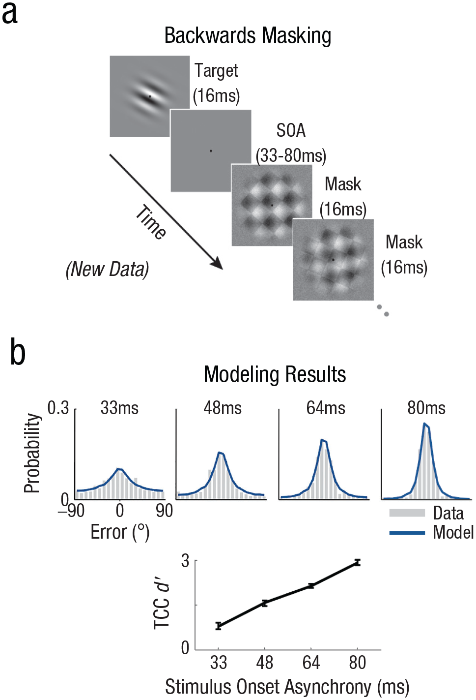
Backwards masking task and model fits to the data. (a) Structure of backward masking paradigm. Note that in the experiment, the target Gabor was shown at lower opacity but is displayed at full opacity for display purposes. (b) Target confusability competition (TCC) fits to group data (N = 15, which was predetermined and based on extensive pilot testing) across the different stimulus onset asynchronies (SOAs). Gray bars signify the error distribution between the target orientation and the response orientation plotted as a function of distance in degrees of error. Blue lines signify the model fit to the continuous report data. The line graph shows TCC d′ on the y-axis and the SOA on the x-axis.

We found that the d′ parameter of the TCC model fit the behavioral errors that participants made quite well and that d′ steadily decreased as the duration between the target and the masks decreased (Fig. 4b), with mean d′ of 2.6, 2.0, 1.4, and 0.7 at lags 83 ms, 67 ms, 50 ms, and 33 ms, respectively. Thus, shorter stimulus onset asynchronies (SOAs) led to noisier representations.

To address the question of whether there were all-or-none failures, we fitted the mixture model and compared it with TCC. In particular, we directly compared the one-parameter TCC model with a two-parameter mixture model (Zhang & Luck, 2008) and found that the TCC model was strongly preferred over the mixture model at every SOA (BIC differences: 33 ms: 48.8, 50 ms: 40.6, 67 ms: 59.4, 83 ms: 46.3). Summing across conditions, we found that the BIC favored TCC in 14 out of 15 participants. This suggests that a model based on noisy representations alone is preferred to one with all-or-none failures. In addition to this comparison between distinct models, it is also possible to take the TCC model and add a guess rate to it, allowing that although TCC may mostly explain the data simply in terms of added representational noise, all-or-none failures may also exist. This model of TCC with guesses was strongly disfavored by the BIC, suggesting that a model based solely on added noise with no additional all-or-none failures was the best fit to the data (BIC differences favoring no guessing: 33 ms: 86.2, 50 ms: 86.7, 67 ms: 86.9, 83 ms: 87.1). The TCC model without guesses was preferred in all participants.

Thus, we found that even in the case of backward masking, considering participants’ responses as arising from continuous degradation of a single underlying strength parameter is a better account of the data than an account that supposes a mixture of some “visible” and some “invisible” trials (i.e., a mixture model).

Sperling paradigm

Although the Sperling paradigm (1960) does not render stimuli invisible, it is one of the most extensively studied perceptual paradigms in consciousness studies. Indeed, it sits at the center of an extensive debate about the capacity limits of perceptual awareness, with some authors arguing that perception is “rich” (Block, 2011; Lamme, 2003; Sligte et al., 2008) and others maintaining that it is “sparse” (Cohen & Dennett, 2011; Dehaene, 2014; Kouider et al., 2010; Phillips, 2011; Sergent et al., 2013). Given its relevance to the study of perceptual awareness, we asked how well the TCC model’s single latent representational strength parameter—as opposed to a mixture of precision errors and discrete failures (e.g., Zhang & Luck, 2008)—could account for performance in this paradigm.

Pratte (2018) used the Sperling paradigm with continuous reproduction of both color and orientation and collected large amounts of data per participant. The color wheel they used was quite distinct from the color wheel for which we had TCC similarity data; therefore, we refitted the data from their orientation experiment (Experiment 2b). In Experiment 2b by Pratte (2018), 10 Gabor patches were briefly shown (200 ms) in a circular configuration (Fig. 5a). After a variable retention interval, a black line cued participants to one of the 10 locations previously occupied by a Gabor. This cue appeared between 33 ms and 1,000 ms after the offset of the initial display, at which time, participants reported the orientation of the target item using continuous reproduction. Pratte then used a two-parameter mixture model to estimate the precision and guess rate of the cued item (Zhang & Luck, 2008). In this study, the author ultimately concluded that iconic memories “die a sudden death” because the guess rate changed over time, whereas the precision of the remembered items remained approximately the same (see Pratte, 2018, Fig. 3). In other words, the modeling results of this experiment were taken to support a discrete, all-or-nothing view of perceptual awareness. Does the TCC model, with just a single strength parameter, fit these data better than the mixture model?

Fig. 5.

Iconic memory task from Pratte (2018) and model fits to the data. (a) Structure of Sperling paradigm. (b) Target confusability competition (TCC) fits to group data (N = 35) across the match and nonmatch conditions. Gray bars signify the error distribution between the target orientation and the response orientation plotted as a function of distance in degrees of error. Blue lines signify the model fit to the continuous report data. The line graph shows TCC d′ on the y-axis and the match/nonmatch conditions on the x-axis.

We found that the one-parameter TCC model accurately fit participants’ responses quite well, with d′ gradually decreasing as the retention interval increased (Fig. 5b), F(7, 42) = 55.9, p < .0001. This is consistent with the idea that longer delays result in noisier representations.

To address the question of whether there were all-or-none failures, we next fitted the two-parameter mixture model and compared it with TCC. We found that the fit of the TCC model was preferred over the mixture model at every retention interval (BIC differences: 33 ms: 46.4, 67 ms: 31.3, 100 ms: 39.2, 150 ms: 45.9, 233 ms: 45.9, 383 ms: 62.5, 617 ms: 53.2, 1,000 ms: 48.9) and across conditions in five of seven participants. Thus, a model based on noisy representations alone is preferred to one with all-or-none failures. In addition to this comparison between distinct models, it is also possible to take the TCC model and add a guess rate to it, allowing that although TCC may mostly explain the data simply in terms of added representational noise, all-or-none failures may also exist. This model of TCC with guesses was strongly disfavored by the BIC, suggesting that a model based solely on added noise with no additional all-or-none failures was the best fit to the data (BIC differences: 33 ms: 55.0, 67 ms: 51.9, 100 ms: 53.8, 150 ms: 52.9, 233 ms: 52.8, 383 ms: 52.1, 617 ms: 52.8, 1,000 ms: 53.2). The TCC model without guesses was preferred in all participants.

Thus, we found that the best account of iconic memory data is that memory strength drops continuously with delay and there is no need to posit discrete failures of perceptual consciousness to account for participants’ patterns of errors.

Retro-cuing

One paradigm closely related to the Sperling paradigm is a retro-cuing paradigm that cues attention after a stimulus disappears and subsequently improves perception of a target at threshold (Sergent et al., 2013). These findings have been cited to support the view that the initial sensory processing of a stimulus can occur subconsciously and then later be elevated into consciousness, consistent with the sparse view of perceptual awareness.

One study by Thibault et al. (2016) combined this paradigm with mixture modeling to ask whether retro-cuing attention increases the frequency of conscious processing—which is seen as discretely occurring or not occurring—or increases the precision of recollection for those items that were consciously processed. In this study, a target Gabor grating was presented in one of two circular placeholders at perceptual threshold (Fig. 6a). This target was either preceded by a pre-cue or followed by a retro-cue, indicated by one of the placeholders being dimmed. The cues could be either valid (i.e., same side as the target) or invalid (i.e., opposite side of the target). After a brief delay, participants were instructed to continuously adjust the orientation of a probe item to match the orientation of the previously seen target. Thibault et al. (2016) then used a two-parameter mixture model to estimate the precision and guess rate of the cued item (Zhang & Luck, 2008). This modeling claimed to show that the benefits to perception from retro-cuing arise by reducing the frequency of guesses, not by changing the precision of responses (see Thibault et al., 2016, Fig. 3). In other words, these modeling results were taken to support a discrete, all-or-nothing view of perceptual awareness. Does the TCC model fit these data better than the mixture model, supporting an alternative, graded view of performance improvement from retro-cues?

Fig. 6.

Retro-cuing task from Thibault et al. (2016) and model fits to the data. (a) Structure of retro-cuing paradigm. (b) Target confusability competition (TCC) fits to group data (N = 20) across the different cuing conditions (i.e., interstimulus intervals, or ISIs). Gray bars signify the error distribution between the target orientation and the response orientation plotted as a function of distance in degrees of error. Blue lines signify the model fit to the continuous report data. The line graph shows TCC d′ on the y-axis and the different ISIs on the x-axis.

We found that the one-parameter TCC model accurately fit participants’ responses quite well, with d′ being higher for the valid cue in the shorter cuing intervals and this effect decreasing as the cue arrives later (Fig. 6b). In particular, we observed a main effect of SOA, F(2, 16) = 15.5, p < .001, a main effect of cue validity, F(1, 32) = 76.3, p < .0001, and an interaction between these two factors, F(2, 32) = 43.1, p < .0001. These results closely matched the model-free (i.e., non-mixture model) analyses done by Thibault et al. (2016; Fig. 4).

To address the question of whether there are all-or-none failures, we then compared the fit of the TCC model with the two-parameter mixture model and found that the fit of the TCC model was preferred over the mixture model at every retention interval in both valid cues (BIC differences: –100 ms: 50.1, 100 ms: 71.8, 1,400 ms: 22.7) and invalid cues (–100 ms: 26.1, 100 ms: 37.5, 1,400 ms: 59.1). Summing across conditions, we found that the BIC favored TCC in 15 out of 17 participants. Thus, a model based on noisy representations alone is preferred to one with all-or-none failures. In addition to this comparison between distinct models, it is also possible to take the TCC model and add a guess rate to it, allowing that although TCC may mostly explain the data simply in terms of added representational noise, all-or-none failures may also exist. This model of TCC with guesses was not at all favored by the BIC, suggesting that a model based solely on added noise with no additional all-or-none failures was the best fit to the data (BIC differences—valid: –100 ms: 123.8, 100 ms: 124.4, 1,400 ms: 122.9; invalid: –100 ms: 122.9, 100 ms: 121.8, 1,400 ms: 120.2). The TCC model without guesses was preferred in all participants.

Thus, simple degradation of performance with delay to the cue, combined with a benefit of valid cues, is sufficient to account for these data without any discrete failures of consciousness or discrete reactivation of items into consciousness.

Across experiments

The fact that the results from the attentional blink, backward masking, iconic memory, and retro-cuing can all be fit by varying a single representational strength parameter appears to falsify the idea that errors in these paradigms represent changes in two psychologically distinct constructs (e.g., precision vs. guess rate). In the current data sets as a whole (71,123 data points), fitting all conditions and subjects separately, mixture models require 876 parameters to fit approximately as well as TCC fits with only 474 parameters, which considered all together gives TCC a BIC advantage of 3487.4. Another way to test this, in line with what was done by Schurgin et al. (2020) for working memory and long-term memory, is to fit the mixture model to data from these data sets in a single stimulus space and plot the guess rate and standard deviation of the results against one another in state-trace plots (Dunn & Kalish, 2018). In this case, the TCC framework posits that as long as the stimulus space is held constant, the perceptual confusion structure is constant, and so the guess rate and standard deviation should always change together along a single continuum. By contrast, the mixture modeling framework posits that precision and guess rate are genuinely separate constructs. Thus, there are many patterns of data possible in a state trace that would strongly falsify TCC by virtue of them simply not falling along the TCC continuum.

Figure 7 shows the state-trace plot for all orientation data, which is the dominant stimulus in the data that we have refit, from the current article (i.e., the 24 conditions using orientation shown above). As can be clearly seen in this plot, the guess rate and standard deviation parameters of the mixture always change together along the zero-free-parameter prediction of TCC (e.g., TCC’s prediction across a range of d′ values). Although their relationship is not linear, they are nearly perfectly related. Again, it should be stressed that any pattern of data that falls far off the TCC continuum would be completely incompatible with TCC. For instance, (a) precise perception but many guesses (the top left corner) or (b) imprecise perception and no guesses (the bottom right corner) could not be accounted for under this framework. These results lend further support to the idea that TCC’s single parameter conception of performance is correct and that mixture models are not measuring distinct psychological constructs. With respect to studies of perceptual awareness, this means that there is no need to posit discrete, all-or-none failures of perceptual access (guesses) to account for the errors that participants make in these paradigms.

Fig. 7.

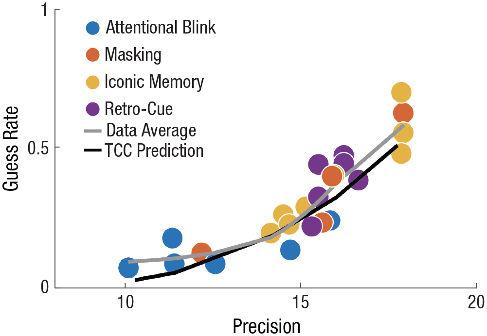
Target confusability competition (TCC) makes a strong counter prediction to mixture models about their own parameters: that if the stimulus space, and thus psychophysical similarity function, is held constant, memory report distributions vary in only one way, in memory strength. To visualize this, we show a state-trace plot of mixture model parameters across the wide range of experimental results that we have refit, focusing only on the orientation data. We found that despite the huge number of different ways that representational strength is varied, all the points lie approximately on a single line, consistent with only a single parameter being varied, which is well predicted by the 0-free-parameter prediction of TCC. TCC can predict only an extremely small part of the possible space that the mixture model can predict, and only a very particular relationship between the two mixture model parameters, and the data from all of these conditions land directly on this line. This provides strong evidence against mixture models measuring two distinct parameters and in favor of the TCC conception of memory. Note that data from the work by Asplund et al. (2014) are not plotted because that experiment used color stimuli, whereas the other experiments used oriented Gabors, and stimuli from different stimuli spaces cannot be put on a single state-trace plot.

Thus, we found that greater standard deviations are associated with greater guess rates, in a predictable nonlinear pattern, and in line with the prediction of the TCC model. Note that this is in the opposite direction from what is predicted by noisy fits to data: Uncertainty or noisy fits in mixture models lead to the reverse of the trend that we report in the current results: Larger standard deviations lead to lower guess rates and vice versa (Suchow et al., 2013, explained that his occurs because the data right at the edge of the “von Mises” part of the mixture model can be seen as either arising from a larger standard deviation or arising because of guesses, resulting in a trade-off between these two parameters with noisy data). Thus, imprecise estimates of these parameters due to insufficient data result in a negative correlation between them, in contrast to the particular positive, nonlinear pattern predicted by TCC that we observe here.

General Discussion

Does information reach perceptual awareness in a continuous or discrete manner? A common tool used to try to answer this question is probabilistic mixture modeling (Zhang & Luck, 2008). This technique separates how often an item does or does not reach awareness (i.e., the guess rate) from how precisely that item is represented in awareness (i.e., the standard deviation), using continuous reproduction tasks. Contrary to this mixture model approach, however, recent work with the TCC model has shown that when one considers the nonlinear way that familiarity spreads through a stimulus space, there is no evidence for separate concepts of precision and guessing (Schurgin et al., 2020). Instead, the TCC model states that memory and perception can be modeled by taking the spread of familiarity through a stimulus space and adding noise, with d′ being the only free parameter. In the current work, we asked how well this continuous model captures responses across a variety of paradigms that manipulate perceptual awareness. Specifically, we reanalyzed data from prior studies (Asplund et al., 2014; Pratte, 2018; Sy et al., 2021; Thibault et al., 2016) and one new backward masking experiment. Across four paradigms and two stimulus classes, we found that the TCC model easily fit the data and outperformed mixture models in every single instance. We also found that across these studies, the putative precision and guess rate parameters were nearly perfectly confounded, always changing together (Fig. 7), as would be expected if there is only a single construct—representational strength—changing as the tasks are made more difficult. Together, these results suggest that a large part of the literature taken to support all-or-none access to awareness does not actually do so and instead supports a framework in which information enters conscious awareness in a continuous manner.

What exactly does it mean for information to reach consciousness along a continuum? Instead of the claim that there is no merit to the discrete, all-or nothing view of perceptual awareness, one unifying possibility is that performance on tasks such as those studied here is more sensitive to the strength of information representation than to whether stimuli have reached “awareness,” which could be an all-or-none state, but one that is not necessary to support performance (Lau & Rosenthal, 2011). For example, consider the backward masking paradigm described above (Fig. 4a). An intuitive description of participants’ experience is that the content of that information varies along a continuum and can be reported regardless of awareness, whereas the mechanisms that allow information to be accessed by awareness could still be all-or-none (i.e., “I am certain I saw something, but I have only a vague sense that it was oriented to the right”). This idea was previously proposed by Kouider et al. (2010), who argued in favor of a “partial awareness” hypothesis in which the representations of an object can be continuous, whereas the mechanisms that allow those representations to be accessed by consciousness are discrete. This particular framework is supported by prior studies showing that observers will sometimes provide “intermediate” reports about the contents of their experience (i.e., a brief glimpse or a vague sense of what was present) when given several options on a perceptual awareness scale (Sandberg et al., 2010). A similar idea has been proposed by Michel (2019), who made a critical distinction between the graded contents of consciousness and graded consciousness overall. Of course, in spite of these claims, there are still those who maintain that consciousness itself (not just the contents of consciousness) is fundamentally graded (Morales, 2021).

In each paradigm examined here, observers frequently felt as if there were instances in which they completely failed to perceive the target and were simply guessing when asked to make a judgment about it. This feeling appears to be captured under a mixture modeling framework because one of the parameters of the model is the guess rate, which is thought to correspond to the instance in which the target was not successfully encoded. However, previous work has shown that this is not accurate: People often give highly confident reports of items that are extremely dissimilar to the actual item (Adam et al., 2017), which mixture models would classify as guesses. The TCC framework, by contrast, is based on signal detection theory, which explains the feeling of guessing as one of low subjective confidence, which is expected to regularly arise when a task is difficult (as modeled by Schurgin et al., 2020). In other words, although TCC claims that there are rarely situations in which an observer has a discrete failure with no information and is objectively guessing, it easily accounts for the subjective feeling of guessing and poor performance—and how they are linked—by appealing to noisy variation in the familiarity signal (Wixted, 2020). This conception of perceptual awareness also helps unite the current behavioral results with established findings from neuroscience. Indeed, one reason that researchers have argued for a discrete view of consciousness is that studies have shown an all-or-none change in neural activity in response to stimuli that observers report having seen, which is not present for unseen stimuli (Dehaene et al., 2001; Sergent & Dehaene, 2004). This nonlinear processing is referred to as the “ignition” of consciousness and is characterized by a sudden, coherent, and exclusive activation of neurons associated with conscious processing (Dehaene, 2014). Under the framework described here, information may be “ignited” into conscious awareness in an all-or-none manner, but the content of what is elevated into consciousness varies along a continuum, and even in the absence of this spark of conscious awareness, noisy information is still accessible for report.

Finally, there are two points worth stressing about TCC’s success in modeling perceptual awareness. First, TCC’s success with these tasks is surprising given the different mechanisms that limit awareness across these paradigms. For example, the attentional blink prevents stimuli from reaching consciousness because of limitations of attention (Raymond et al., 1992), whereas masking renders stimuli invisible by disrupting feedback between higher and lower level visual areas (Lamme, 2003). In addition, the attentional blink is a limitation across time, whereas the Sperling paradigm is more limited across space (Pratte, 2018). The fact that behavioral performance across these tasks is captured by TCC is a testament to the versatility of an approach based on continuous variation in a population of signals in understanding visual cognition. Moreover, TCC’s success with these perceptual tasks was not a given considering that it was initially conceived as a model of visual memory (Schurgin et al., 2020). Altogether, this collection of results highlights how a simple signal detection theoretic framework can capture numerous aspects of human cognition.

Supplemental Material

sj-pdf-1-pss-10.1177_09567976231186798 – Supplemental material for Perceptual Awareness Occurs Along a Graded Continuum: No Evidence of All-or-None Failures in Continuous Reproduction Tasks

Supplemental material, sj-pdf-1-pss-10.1177_09567976231186798 for Perceptual Awareness Occurs Along a Graded Continuum: No Evidence of All-or-None Failures in Continuous Reproduction Tasks by Michael A. Cohen, Jonathan Keefe and Timothy F. Brady in Psychological Science

Footnotes

Transparency

Action Editor: Rachael Jack

Editor: Patricia J. Bauer

Author Contribution(s)

Michael A. Cohen: Conceptualization; Data curation; Formal analysis; Funding acquisition; Investigation; Methodology; Project administration; Visualization; Writing – original draft.

Jonathan Keefe: Conceptualization; Data curation; Formal analysis; Investigation; Writing – review & editing.

Timothy F. Brady: Conceptualization; Data curation; Formal analysis; Funding acquisition; Investigation; Methodology; Resources; Software; Validation; Writing – review & editing.

ORCID iDs

Michael A. Cohen

Jonathan Keefe

Supplemental Material

Additional supporting information can be found at

References

Adam

K. C. S.

Vogel

E. K.

Awh

(2017). Clear evidence for item limits in visual working memory. Cognitive Psychology, 97, 79–97.

Asplund

C. L.

Fougnie

Zughni

Martin

J. W.

Marois

(2014). The attentional blink reveals the probabilistic nature of discrete conscious perception. Psychological Science, 25(3), 824–831.

Bays

P. M.

(2014). Noise in neural populations accounts for errors in working memory. Journal of Neuroscience, 34, 8502–8511.

Bays

P. M.

Catalao

R. F. G.

Husain

(2009). The precision of visual working memory is set by allocation of a shared resource. Journal of Vision, 9(10), Article 7. https://doi.org/10.1167/9.10.7

Block

(2011). Perceptual consciousness overflows cognitive access. Trends in Cognitive Sciences, 15, 567–575.

Brady

T. F.

Konkle

Gill

Oliva

Alvarez

G. A.

(2013). Visual long-term memory has the same limit on fidelity as visual working memory. Psychological Science, 24, 981–990.

Carruthers

(2019). Human and animal minds: The consciousness questions laid to rest. Oxford University Press.

Cohen

M. A.

Dennett

(2011). Consciousness cannot be separated from function. Trends in Cognitive Sciences, 15, 358–364.

Dehaene

(2014). Consciousness and the brain: Deciphering how the brain codes our thoughts. Penguin Books.

10.

Dehaene

Naccache

Cohen

Bihan

D. L.

Mangin

J. F.

Poline

J. B.

Riviere

(2001). Cerebral mechanisms of word masking and unconscious repetition priming. Nature Neuroscience, 4, 752–758.

11.

Dunn

J. C.

Kalish

M. L.

(2018). State-trace analysis. Springer Press.

12.

Elliott

J. C.

Baird

Giesbrecht

(2016). Consciousness isn’t all-or-none: Evidence for partial awareness during the attentional blink. Consciousness and Cognition, 40, 79–85.

13.

Golomb

J. D.

L’Heureux

Z. E.

Kanwisher

(2014). Feature-binding errors after eye movements and shifts of attention. Psychological Science, 25, 1067–1078.

14.

Kouider

de Gardelle

Sackur

Dupoux

(2010). How rich is consciousness? The partial awareness hypothesis. Trends in Cognitive Sciences, 14, 301–307.

15.

Kouider

Dehaene

(2007). Levels of processing during non-conscious perception: A critical review. Philosophical Transactions of the Royal Society B, 362, 857–875.

16.

Lamme

(2003). Why visual attention and awareness are different. Trends in Cognitive Sciences, 7, 12–18.

17.

Lau

Rosenthal

(2011). Empirical support for higher-order theories of conscious awareness. Trends in Cognitive Sciences, 15, 365–373.

18.

MacMillan

N. A.

Creelman

D. C.

(1991). Detection theory: A user’s guide. Cambridge University Press.

19.

Michel

(2019). The mismeasure of consciousness: A problem of coordination for the Perceptual Awareness Scale. Philosophy of Science, 86, 1239–1249.

20.

Morales

(2021). Introspection is signal detection. British Journal for the Philosophy of Science. Advance online publication. https://doi.org/10.1086/715184

21.

Nieuwenhuis

de Kleijn

(2011). Consciousness of targets during the attentional blink: A gradual or all-or-none dimension? Attention, Perception, and Psychophysics, 73, 364–373.

22.

Overgaard

Rote

Mouridsen

Ramsøy

T. Z.

(2006). Is conscious perception gradual or dichotomous? A comparison of report methodologies during a visual task. Consciousness and Cognition, 15, 700–708.

23.

Phillips

I. B.

(2011). Perception and iconic memory: What Sperling doesn’t show. Mind and Language, 26, 381–411.

24.

Phillips

I. B.

(2020). Blindsight is qualitatively degraded conscious vision. Psychological Review, 128, 558–5843.

25.

Pratte

M. S.

(2018). Iconic memories die a sudden death. Psychological Science, 29, 877–887.

26.

Raymond

J. E.

Shapiro

K. L.

Arnell

K. M.

(1992). Temporary suppression of visual processing in an RSVP task: An attentional blink? Journal of Experimental Psychology: Human Perception and Performance, 18, 849–860.

27.

Roberts

Pashler

(2000). How persuasive is a good fit? A comment on theory testing. Psychological Review, 107, 358–367.

28.

Salahub

C. M.

Emrich

S. M.

(2016). Tuning perception: Visual working memory biases the quality of visual awareness. Psychonomic Bulletin and Review, 23, 1854–1859.

29.

Sandberg

Timmermans

Overgaard

Cleermans

(2010). Measuring consciousness: Is one measure better than the other? Consciousness and Cognition, 19, 1069–1078.

30.

Schurgin

M. W.

Wixted

J. T.

Brady

T. F.

(2020). Psychophysical scaling reveals a unified theory of visual memory strength. Nature Human Behaviour, 4, 1156–1172.

31.

Schwarz

(1978). Estimating the dimension of a model. Annals of Statistics, 6, 461–464.

32.

Sergent

Dehaene

(2004). Is consciousness a gradual phenomenon? Evidence for an all-or-none bifurcation during the attentional blink. Psychological Science, 15, 720–728.

33.

Sergent

Wyart

Babo-Rebelo

Cohen

Naccache

Tallon-Baudry

(2013). Cueing attention after the stimulus is gone can retrospectively trigger conscious perception. Current Biology, 23, 150–155.

34.

Sligte

I. G.

Scholte

H. S.

Lamme

V. A. F.

(2008). Are there multiple visual short-term memory stores? PLOS ONE, 3, Article e1699. https://doi.org/10.1371/journal.pone.0001699

35.

Suchow

J. W.

Brady

T. F.

Fougnie

Alvarez

G. A.

(2013) Modeling visual working memory with the MemToolbox. Journal of Vision, 13, 9.

36.

J. L.

Miao

H.-Y.

Marois

Tong

(2021). Conscious perception can be both graded and discrete. Journal of Experimental Psychology: General, 150, 1461–1475.

37.

Thibault

van den Berg

Cavanagh

Sergent

(2016). Retrospective attention gates discrete conscious access to past sensory stimuli. PLOS ONE, 11(2), Article e0148504. https://doi.org/10.1371/journal.pone.0148504

38.

van den Berg

Shin

Chou

W. C.

George

W. J

. (2012). Variability in encoding precision accounts for visual short-term memory limitations. Proceedings of the National Academy of Sciences, USA, 109, 8780–8785.

39.

Vul

Hanus

Kanwisher

(2009). Attention as inference: Selection is probabilistic; responses are all-or-none samples. Journal of Experimental Psychology: General, 138, 546–560.

40.

Williams

J. R.

Brady

T. F.

Störmer

V. S.

(2022). Guidance of attention by working memory is a matter of representational fidelity. Journal of Experimental Psychology: Human Perception and Performance, 48, 1–30.

41.

Williams

J. R.

Robinson

M. M.

Brady

T. F.

(2023). There is no theory-free measure of “swaps” in visual working memory experiments. Computational Brain & Behavior, 6(2), 159–171.

42.

Wixted

J. T.

(2020). The forgotten history of signal detection theory. Journal of Experimental Psychology: Learning, Memory, and Cognition, 46(2), 201–233.

43.

Zhang

Luck

S. J.

(2008). Discrete fixed-resolution representations in visual working memory. Nature, 453, 233–235.

Supplementary Material

Please find the following supplemental material available below.

For Open Access articles published under a Creative Commons License, all supplemental material carries the same license as the article it is associated with.

For non-Open Access articles published, all supplemental material carries a non-exclusive license, and permission requests for re-use of supplemental material or any part of supplemental material shall be sent directly to the copyright owner as specified in the copyright notice associated with the article.

0.00 MB

0.52 MB