Comparison of non-linear vibration of outer race defective ball bearing using two defect functions

Abstract

The aim of this article is to study the effects of evolution in defect size on vibration of a ball bearing by simulation of a ball bearing by developing a 2-DOF mathematical model and to compare the vibration responses of defective bearings obtained for two widely used defect functions, viz., rectangular function and half-sine wave function. MATLAB codes are developed to prepare a mathematical model of a ball bearing and to solve the differential equations of the model using the Runge-Kutta method. In the model, the mass supported by the bearing is considered as a lumped mass, and the contact between the races and the balls is considered as a series of springs, whose spring stiffness is obtained by using Hertz’s contact deformation theory. This model considers the contact deformation between the balls and the races and the additional displacement between the balls and the inner race due to radial clearance and defect geometry. The maximum possible radial displacement of the ball into the defect is obtained analytically and graphically from the race-ball-defect geometry. First, the impulses generated due to an outer race defect in the ball bearing are modeled using two different defect functions separately and their vibration responses are compared. Secondly, the effects of increase in defect length on vibration of the bearing are simulated separately for two defect functions, and then their responses are compared and analyzed. The results show that when the defect is modeled with a rectangular defect function, the vibration responses obtained are greater than when the defect is modeled with a half-sine wave defect function. And, vibration responses increase rapidly up to a certain level of defect length and then decrease with a further increase in defect length. The vibration analysis performed for different defect lengths can provide good support to vibration analysts and researchers.

Keywords

Mathematical modeling outer race defects vibration analysis of bearing Hertz’s contact deformation theory simulation Runge-Kutta method

Introduction

Single deep groove ball bearings are widely used in rotating machinery, running at high speeds, such as electric motors, fans, turbines, compressors, automobiles, etc. Generally, bearing’s inner race is mounted on the shaft, its outer race is fixed in the housing, and a series of balls are placed in between the two races to separate them and reduce friction. Defects on these elements may cause catastrophic damage and hence need to be detected in their incipient stages before they become serious. Bearing defects fall into two broad categories, localized and distributed. Localized defects on the bearing surface include cracks, pits, bumps, and dents, while distributed defects include waviness, misaligned races, roughness, and odd-sized rolling elements.^1–4

In traditional experimental methods, to understand the effects of bearing defects under different conditions, the vibration signals of the bearings are obtained by incorporating defects artificially in them or waiting for the defects to take place in the bearing naturally, but this process is costly and lengthy. Modeling and simulation reduce the time and cost. Modeling of bearings with defects makes it possible to easily study in detail the effects of defects under different conditions in less time, and it also helps to understand the seriousness of the defects developed in the bearings. As a result, vibration analysts are strongly interested in understanding the dynamic behavior of bearings that result from defects, leading to the development of mathematical models. Recently, some researchers^5–10 have reviewed the literature on dynamic modeling and simulation of vibration caused by localized and distributed defects on Rolling element bearings (REBs). These review articles reveal that among different models, such as finite element models, impulse train models, and non-linear dynamic mathematical models (NDMMs), the NDMMs are the most commonly used models by researchers for modeling bearings with distributed and localized defects. REBs experience non-linear vibration primarily due to contact forces, radial clearance, varying compliance, defects, preloading, unbalance, and damping.¹⁰ While modeling the bearings using NDMMs, researchers used Hertzian contact deformation theory to determine the contact forces between the races and the balls.¹¹

The NDMMs used by the researchers for modeling bearings with defects and associated systems can be classified into three categories: modeling of the bearing system, modeling of the bearing-housing system and modeling of the rotor-bearing system. In the modeling of a bearing system, the mass supported by the bearing is considered a lumped mass; however, while modeling of bearing-housing systems and rotor-bearing systems, the masses of housing and rotor system (shaft and disk) respectively are considered along with the mass supported by the bearing.

In the last two decades, many researchers^12–30 developed NDMMs for bearing systems that involve single-row DGBBs having an individual localized defect or compound defects on one of the bearings. These ball bearing systems are modeled by using 2-DOF models and by assuming that the rotating bearing elements have only two-directional (planar) motions. Most of the researchers modeled the bearing defects using a rectangular function or a half-sine wave function. They used the Runge-Kutta method or Newmark-β method for solving the non-linear 2^nd order differential equations of motion.

Rafsanjani et al.¹² developed a model of SKF 6205-2RSL JEM DGBB with localized ORD, IRD, and BD, and studied their effects on bearing vibration responses at different speeds and radial clearances. They observed that the obtained defect frequencies slightly deviate from the calculated frequencies due to the skidding and slipping of the balls. Patil et al.¹³ modeled SKF 6305 DGBB and studied the effects of localized ORD and IRD at different lengths and ORD positions on bearing vibration response. They observed that maximum vibration occurs when the ORD is at the maximum load zone. Kankar et al.¹⁴ modeled a 6002 DGBB with localized ORD, IRD, and BD. They found nonlinear dynamic responses at a higher speed due to localized ORD and IRD. Later, Kankar et al.¹⁵ used the same model and studied the effects of localized ORD, IRD, and BD at different speeds. They showed various unstable and chaotic regions due to localized defects using bifurcation diagrams. Liu et al.¹⁶ developed a ball-bearing model to analyze the effects of localized ORD and its sizes. They modeled the defects as a piecewise response function, in which the combination of rectangular function and half-sine wave function is used. They conclude that the ratio of length to width of the local defects has a significant influence on impulses of time waveform. Later, Liu and Shao¹⁷ studied the effects of defect edge topographies of localized ORD and IRD and their sizes. They observed that contact stiffness increases with the number of defect contact surfaces. Li et al.¹⁸ used and compared the 2-DOF model and 6-DOF model of a SKF 6205 DGBB to study the effects of localized ORD and IRD on bearing vibration response. In their comparison, they found that the 6-DOF model can detect early weak localized defects. Pandya et al.¹⁹ modeled SKF 6205 DGBB with combined localized ORD, IRD, and BD and studied their effects on bearing vibration at different speeds. For combined defects, significant peaks are found at the interaction of defect frequencies and rotational frequencies. Kulkarni et al.²⁰ modeled a 6205 DGBB with localized ORDs and studied the effects of ORD size, ORD position, multiple ORDs and change in load on vibration responses. They used a cubic Hermite spline function to model the defect. They observed that the vibration amplitude increases with an increase in the size of the ORD and when two ORDs are present. Liu et al.²¹ modeled a ball bearing and studied the effects of ORD and IRD, and their sizes on bearing vibration. They observed that when defect size increases, the RMS value increases and kurtosis decreases. Luo and Guo²² modeled a 6205 DGBB to describe the dual-impulse behavior of the ball due to ORD. They investigated the interval of time of double-impulse behavior due to ORD. Yang et al.²³ modeled a 6312 DGBB with localized ORD. They found that variance compliance frequency is the same as ORD frequency. Liu et al.²⁴ modeled a DGBB with combined localized ORD with different defect sizes and surface waviness. They found that the combined defects have a greater influence on vibration amplitude than a single defect and vibration increases as defect size increases. Liu et al.²⁵ modeled a DGBB with dents on its races and studied the effects of dent size on vibrations. They observed that the vibration amplitudes are higher for a dent having a shoulder than a shoulder-less dent. Liu et al.²⁶ modeled a 6308 DGBB with localized ORD with different orientations. They used a piecewise response function for defect modeling. They observed that offset distance and bias angle of local defects affect the impulses and energy of the bearing system. Cheng et al.²⁷ modeled a SKF 6205 DGBB with individual localized ORD, IRD and BD. Li et al.²⁸ proposed an asymptotic defect model for a SKF 6205 DGBB to study the effects of a localized IRD considering the asymptotic change of ball displacement. They also compared the results of the transient model and asymptotic model at different speeds and IRD sizes. Qin et al.²⁹ studied the effects of ORD size and shaft speed on bearing vibration using a 2-DOF model. They used rectangular, half-sine wave and piecewise functions for modeling the ORD functions of the DGBB similar to Liu et al.¹⁶ Fengling et al.³⁰ modeled the SKF 6205 DGBB and studied the effects of a localized IRD and its length on bearing vibrations. They have also studied the effects of changes in speed, radial load, and defect length on various time-domain statistical parameters. They observed that in the early stages, the statistical parameters are sensitive to the IRD length and increase as the defect length increases. However, sensitivity is not significant at different speeds. Jain and Bhosle³¹ modeled a SKF 6205-2RS JEM ball bearing and simulated the effects of radial clearance and number of balls on bearing vibration. They observed that an increase in radial clearance raises the vibration level and an increase in the number of balls lowers the vibration level. Kumbhar et al.³² recently reviewed the latest literature on dynamic modeling of REBs.

In this paper, a 2-DOF non-linear mathematical model of a SKF 6305 DGBB is developed based on Hertz’s contact deformation theory to simulate and analyze the effects of individual localized ORD and its length on bearing vibration responses. Vibration responses like peak-to-peak displacement, peak-to-peak acceleration, RMS acceleration, and peak amplitude of acceleration in the envelope spectrum are obtained in the vertical direction. The model is prepared by considering the contact deformation between the balls and the races, the additional displacement of the balls, and the inner race due to radial clearance and due to defect geometry. The literature review reveals that most of the researchers modeled the bearing defects using a rectangular function or a half-sine wave function. The novel aspect of this work is that both these commonly used defect functions are used for modeling a bearing with an outer race defect, and their vibration responses are compared. The maximum possible radial displacement of a ball into the defect is calculated analytically from the outer race-ball-defect geometry by considering both the outer race and ball radii. This analytical calculation is visually validated through graphical verification using Solid Edge software. The results of modeling and simulation of the bearing are compared by plotting of orbit plots, time waveforms, frequency spectrums and envelope spectrums.

The results of the developed model are validated by comparing the results of other researchers. In the appendix, the summary of the latest literature on 2-DOF modeling of DGBBs with localized defects is also provided.

Modeling of DGBB with localized outer race defect

Bearing input parameters and assumptions

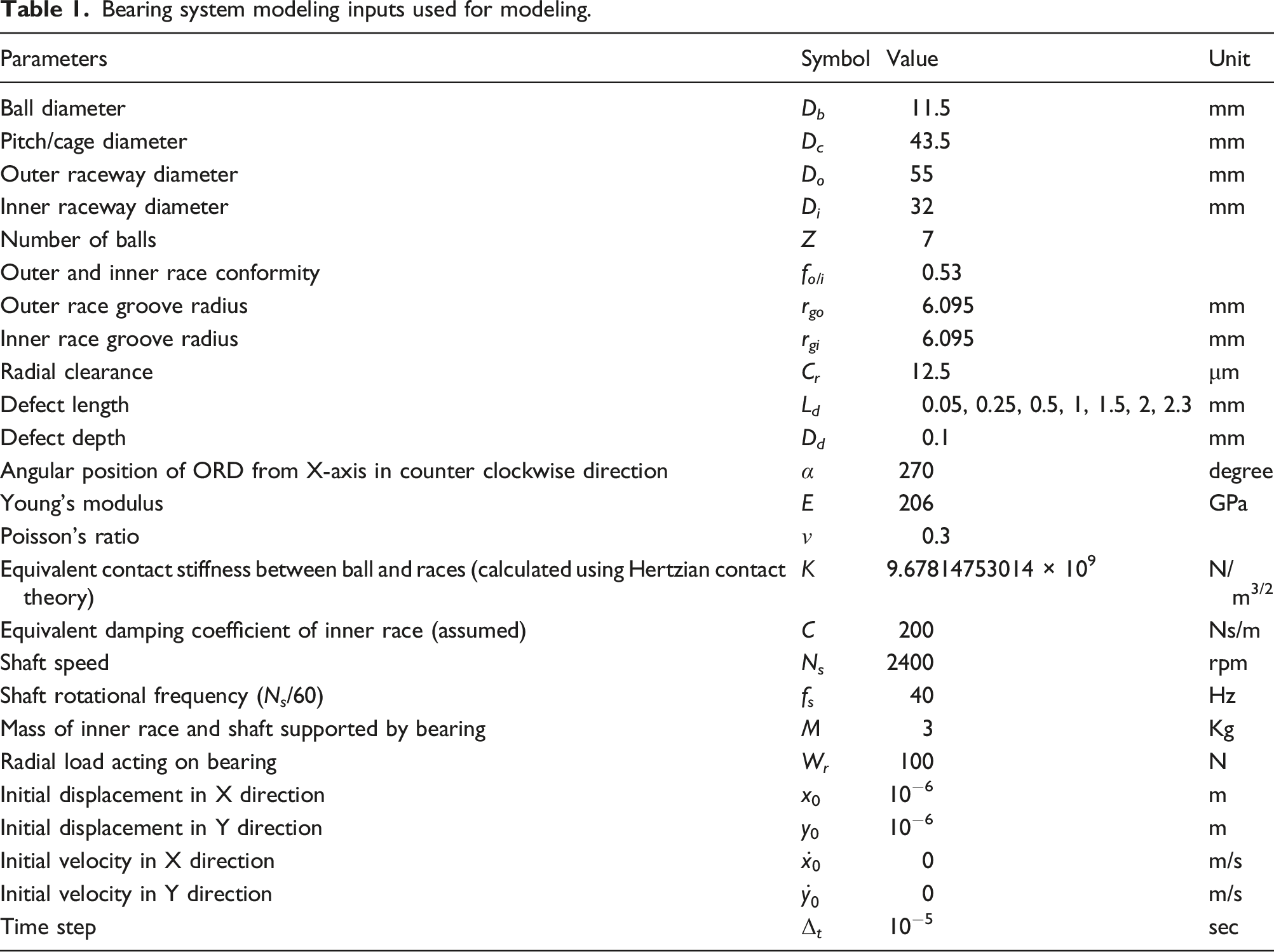
In this study, a SKF 6305 DGBB is modeled with a localized outer race defect by considering different defect lengths. Figure 1 shows a schematic diagram of a SKF 6305 DGBB with some of the important dimensions, and Table 1 shows the details of the input parameters of the bearing system used for modeling.

Figure 1.

Schematic diagrams of SKF 6305 DGBB

Table 1.

Bearing system modeling inputs used for modeling.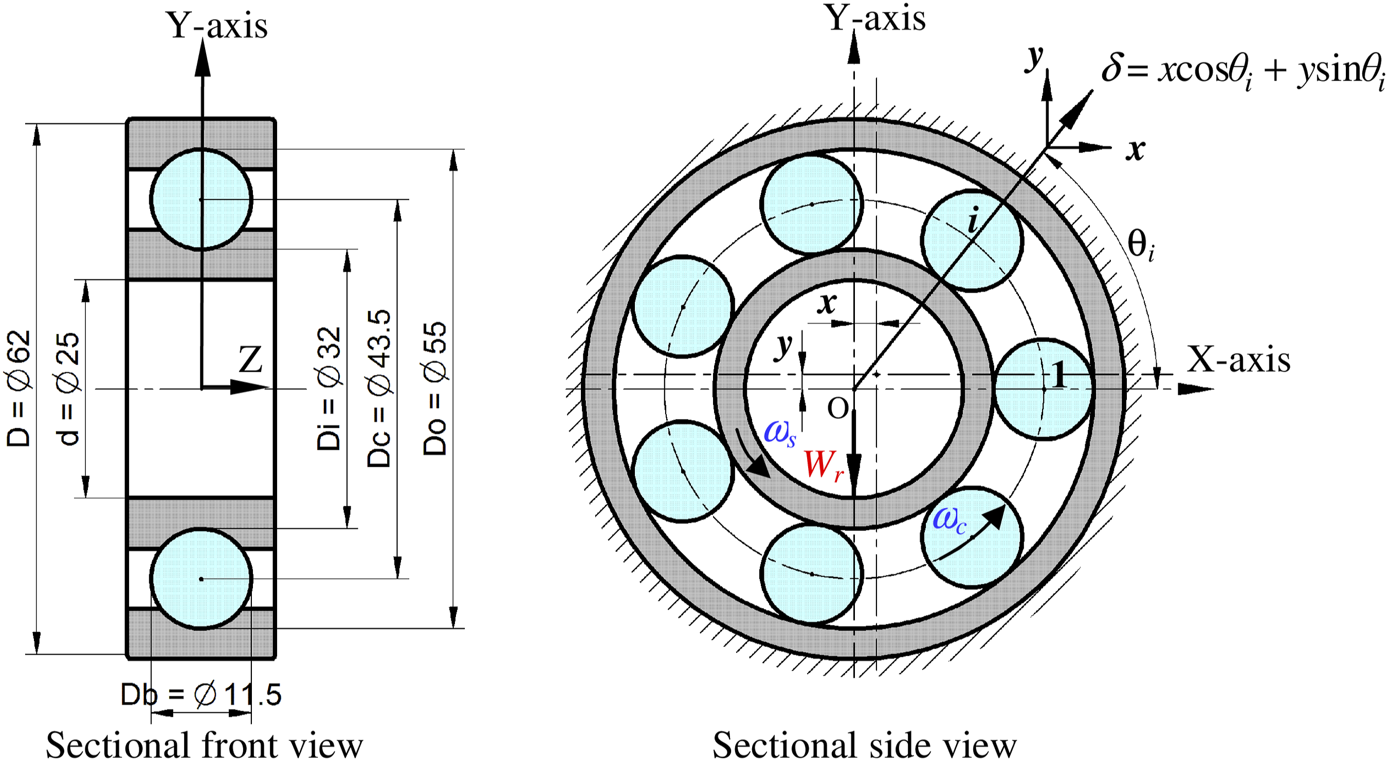

Parameters	Symbol	Value	Unit
Ball diameter	D _b	11.5	mm
Pitch/cage diameter	D _c	43.5	mm
Outer raceway diameter	D _o	55	mm
Inner raceway diameter	D _i	32	mm
Number of balls	Z	7
Outer and inner race conformity	f _o/i	0.53
Outer race groove radius	r _go	6.095	mm
Inner race groove radius	r _gi	6.095	mm
Radial clearance	C _r	12.5	μm
Defect length	L _d	0.05, 0.25, 0.5, 1, 1.5, 2, 2.3	mm
Defect depth	D _d	0.1	mm
Angular position of ORD from X-axis in counter clockwise direction	α	270	degree
Young’s modulus	E	206	GPa
Poisson’s ratio	ν	0.3
Equivalent contact stiffness between ball and races (calculated using Hertzian contact theory)	K	9.67814753014 × 10⁹	N/m^3/2
Equivalent damping coefficient of inner race (assumed)	C	200	Ns/m
Shaft speed	N _s	2400	rpm
Shaft rotational frequency (N_s/60)	f _s	40	Hz
Mass of inner race and shaft supported by bearing	M	3	Kg
Radial load acting on bearing	W _r	100	N
Initial displacement in X direction	x ₀	10⁻⁶	m
Initial displacement in Y direction	y ₀	10⁻⁶	m
Initial velocity in X direction	${\dot{x}}_{0}$	0	m/s
Initial velocity in Y direction	${\dot{y}}_{0}$	0	m/s
Time step	Δ_t	10⁻⁵	sec

In developing the bearing model, some considerations and assumptions are listed below. (1) Outer race is firmly fixed and the inner race is rotating along with the shaft, (2) Mass supported by the bearing is considered as a lumped mass, (3) The contact deformation between the balls and the races are obtained by Hertzian contact deformation theory, (4) Contact stiffness and damping coefficient are assumed as constant, (5) There is no slipping of the balls in the races, (6) Balls are always equally spaced, (7) Masses of balls, cage and housing are neglected, (8) Gyroscopic effects of rotating elements are neglected, (9) All rotational motions are about Z-axis and translational motions are in X and Y plane, (10) Axial clearance and lubrication are neglected and (11) Defect width is along the full width of the bearing.

Calculation of contact deformation $δ$

Figure 1 shows two views of a SKF 6305 DGBB, whose outer race is firmly fixed in the rigid housing and the inner race is firmly fixed on the shaft, which is rotating in a counter-clockwise direction along the Z-axis at a constant speed N_s. A constant radial load W_r is acting on the inner race in the downward direction. The deflections of the center of inner race O in X and Y directions are x and y respectively when the i^th ball makes an angle of θ_i with X-axis. This angle θ_i is given by

θ_{i} = ω_{c} t + \frac{2 π (i - 1)}{Z} + θ_{0}

(1)

where i is the ball number (i = 1, 2, …Z), θ₀ = 0 as 1^st ball is along X-axis, and

ω_{c}

is the cage angular velocity, which is equal to ball angular velocity about O and is given by

ω_{c} = \frac{ω_{s}}{2} (1 - \frac{D_{b}}{D_{c}})

(2)

where

ω_{s}

is the angular velocity of the shaft which is given by

ω_{s} = 2 π N_{s} / 60

Now, the radial contact deformation δ of the i^th ball for any ball angular position θ_i from the X-axis is given by

δ = x \cos θ_{i} + y \sin θ_{i}

(3)

In this study, a localized ORD on SKF 6305 DGBB is considered in the maximum load zone as shown in Figure 2. Since the outer race is rigidly fixed in the housing, the position of the ORD is fixed. Let α be the fixed angle of the center of the ORD from the X-axis in the counter-clockwise direction. Here α = 270^O. If L_d and D_d are the defect length and defect depth respectively, then from the geometry, the angle spanned by the ORD at the outer race center O can be obtained as

ϕ = 2 \sin^{- 1} (\frac{L_{d}}{2 R_{o}})

(4)

Figure 2.

Ball and ORD geometry for analytical calculation of D_max (not true scale).

If the time-varying angular position of a ball from the X-axis (θ_i) is the same as the fixed angular position of the ORD from the X-axis (α) i.e. θ_i = α = 270° as shown in Figure 2, then the ball is at its fully displaced position. In this study, the defect sizes are considered such that the balls do not touch the bottom of ORD at any instance, i.e., the maximum possible radial displacement of a ball into the defect (D_max) is less than the actual defect depth i.e. D_max < D_d.

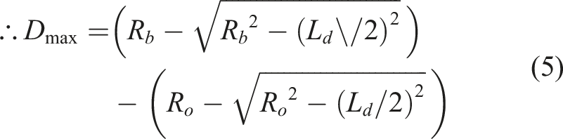
Figure 2 shows the ball and ORD geometry for the calculation of D_max by considering the radius of ball R_b and the radius of outer race R_o. From the geometry,

D_{\max} = BC = AC - AB = (PC - PA) - (OB - OA)

∴ D_{\max} = (R_{b} - \sqrt{{R_{b}}^{2} - {(L_{d} \ / 2)}^{2}}) - (R_{o} - \sqrt{{R_{o}}^{2} - {(L_{d} / 2)}^{2}})

(5)

The ORD lengths (L_d) considered in this study are 0.05, 0.25, 0.5, 1, 1.5, 2 and 2.3 mm. For L_d = 1.5 mm, the value of D_max obtained from equation (5) is 0.03889 mm. Also, from the geometry drawn using Solid Edge V19 software for the ORD having a defect length of 1.5 mm and defect depth of 0.1 mm as shown in Figure 3, the value of D_max obtained is 0.03889 mm. Similarly, for all the ORD lengths considered in this study, the values of D_max are calculated from equation (5) and also obtained using Solid Edge software. These values of D_max are given in Table 2. Since all these values of D_max are less than the total defect depth (D_d = 0.1 mm), it is clear that none of the balls touches the bottom of the ORD at any time since D_max < D_d. Such analysis was not done by Patil et al.¹³ in their study. They used total defect depth (0.1 mm) as the maximum possible radial displacement of a ball into the defect for each defect length.

Figure 3.

Ball and ORD geometry for graphical measurement of D_max (Scale 20:1).

Table 2.

Values of D_max for different defect lengths used in this study.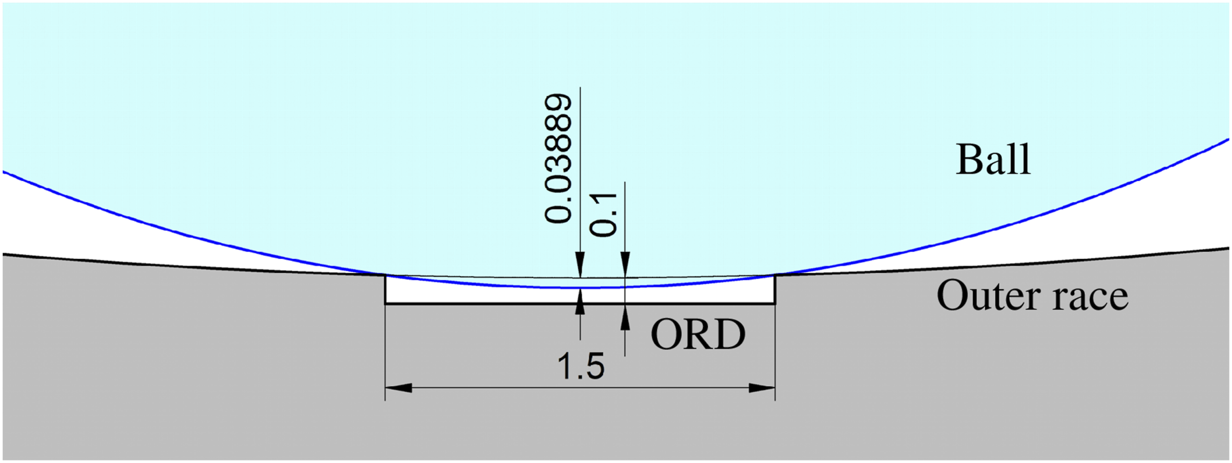

L_d (mm)	0.05	0.25	0.5	1	1.5	2	2.3
D_max (mm)	0.00004	0.00107	0.0043	0.01723	0.03889	0.06943	0.09211

Let Δ_d be the time-varying radial displacement of the ball into the defect, which depends on the function used for modeling the ball center path in the defect zone. In this study, for modeling the ORD, i.e., for modeling the path of the ball center while travelling over the defect zone, two functions, namely the rectangular function (RF) and the half-sine wave function (HSWF) are used, and then their vibration responses are compared. In the rectangular function, it is assumed that the ball center deviates from its circular path and travels through an additional rectangular-shaped path when the ball travels over the ORD zone, as shown by the pink path in Figure 4. And, in the half-sine wave function, it is assumed that the ball center deviates from its circular path and travels through an additional half-sine wave curve path when the ball travels over the ORD zone, as shown by the blue path in Figure 4.

Figure 4.

Different paths of ball center due to displacement of ball in the ORD (not true scale).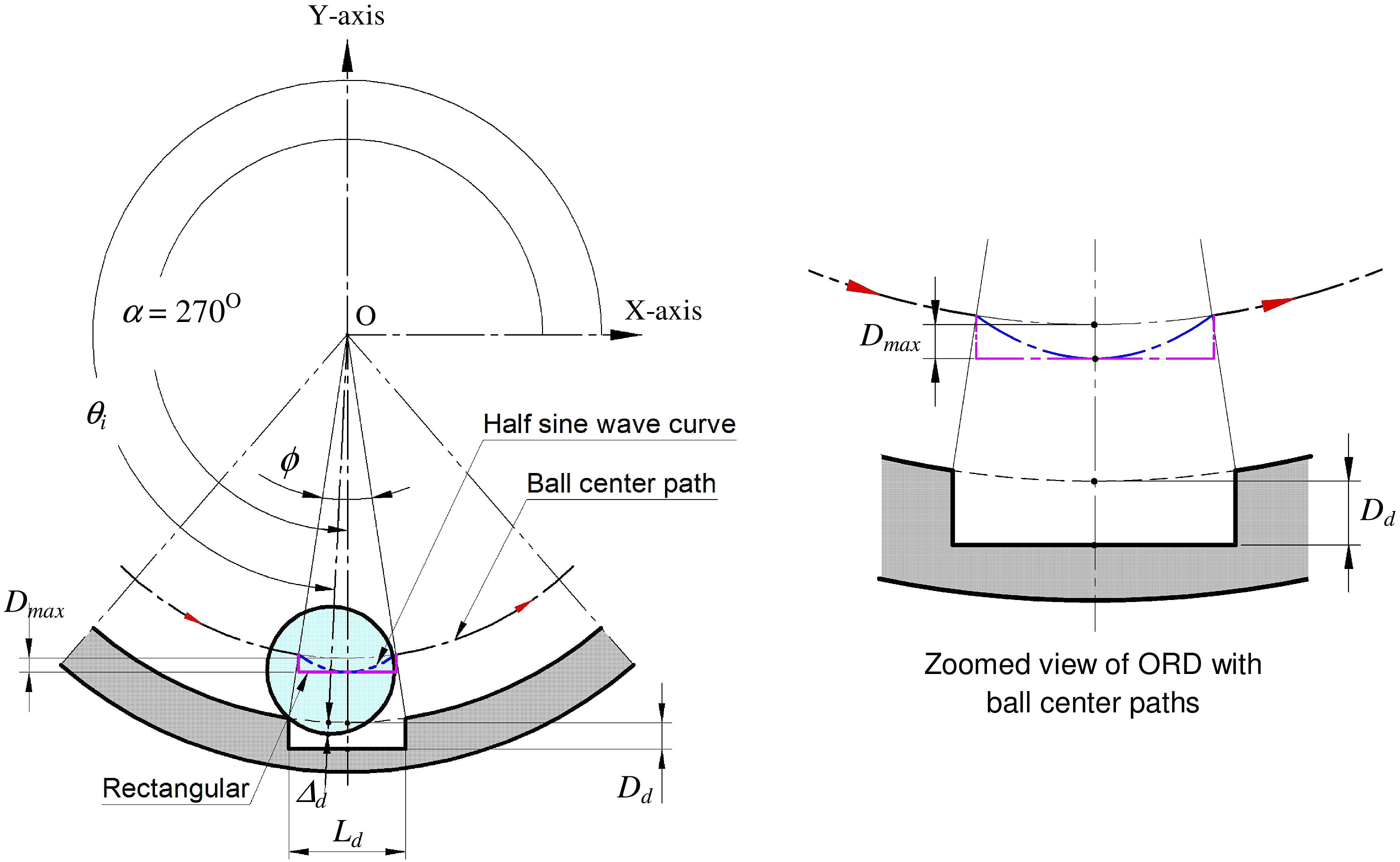

When the ORD is modeled as a rectangular function, then the time-varying radial displacement of the ball into the defect (Δ_d) for any angular position of ball θ_i is

Δ_{d} = D_{\max}

(6)

and when the ORD is modeled as a half-sine wave function, then the time-varying radial displacement of the ball into the defect (Δ_d) for any angular position of ball θ_i is

Δ_{d} = D_{\max} \sin [\frac{π}{φ} (\mod (θ_{i}, 2 π) - (α - \frac{φ}{2}))]

(7)

If radial clearance and a localized ORD are present in the bearing, then these factors reduce some amount of contact deformation of the ball when the ball travels over the ORD zone. Then, the overall radial contact deformation δ of the i^th ball for any ball angular position θ_i is given by

δ = (x \cos θ_{i} + y \sin θ_{i}) - C_{r} - β Δ_{d}

(8)

where C_r is the radial clearance, β is the switch function which is equal to 1 when the ball travels into the defect; otherwise, it is equal to 0. Mathematically,

β = {\begin{cases} 1 & (α - \frac{φ}{2}) < \mod (θ_{i}, 2 π) < (α + \frac{φ}{2}) \\ 0 & otherwise \end{cases}

(9)

Equivalent contact stiffness K between ball and races, and damping coefficient C of the inner race

Figure 5 shows a simplified model of a SKF 6305 DGBB by considering the mass of the inner race and the shaft supported by the bearing as a lumped mass M, and the contacts between the races and the balls as a series of springs according to Hertzian contact deformation theory. Here, K and C are the equivalent contact stiffness (or equivalent load-deflection factor) and the equivalent damping coefficient of the inner race, respectively.

Figure 5.

A simplified model of 6305 bearing.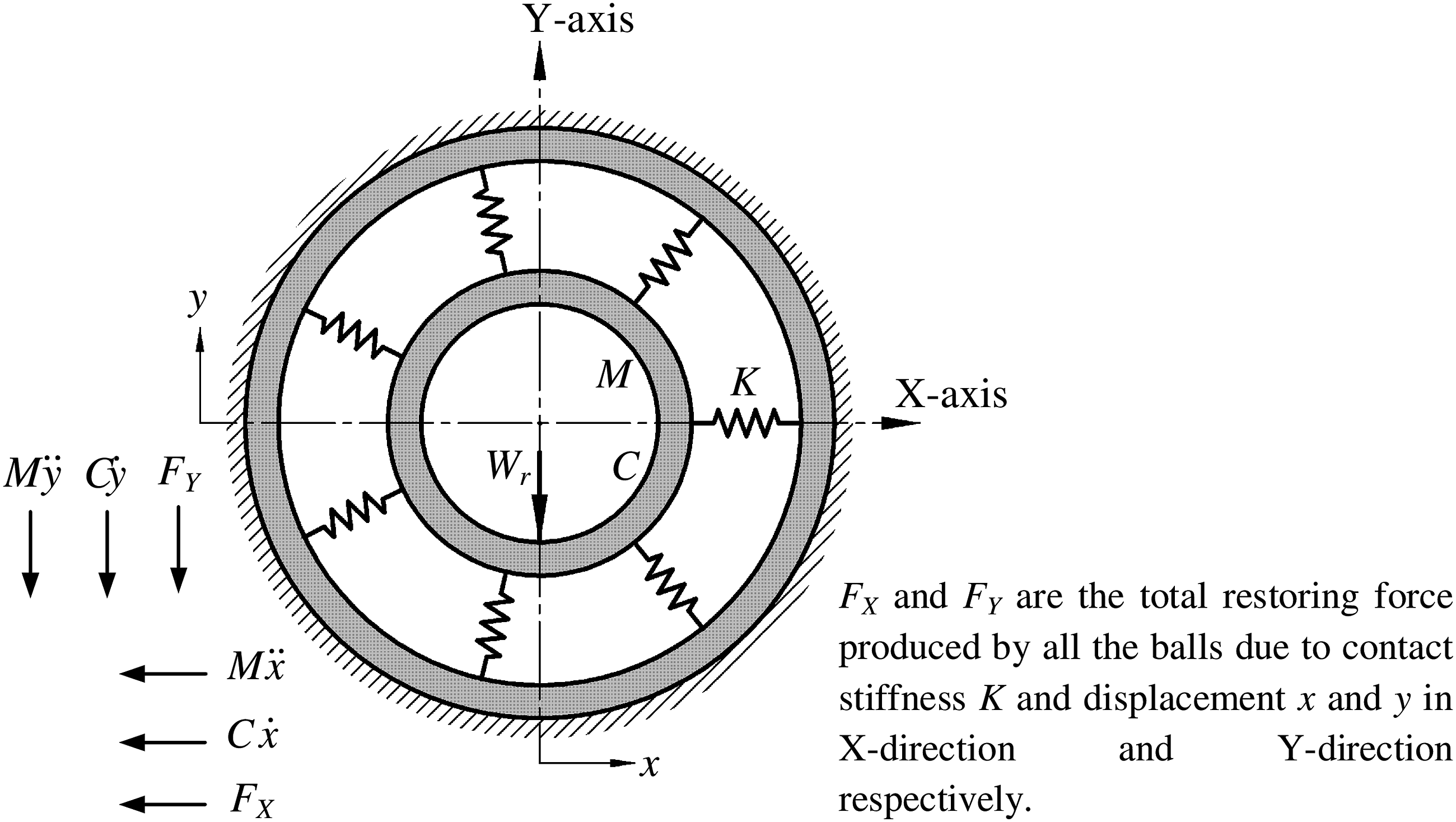

In this study, the constant equivalent contact stiffness K between ball and races in terms of elliptic integrals and ellipticity parameters is obtained by using Hertzian contact deformation theory. This theory is explained by Harris³³ and used by some researchers^{12,17,22,24,34,35} in their studies to calculate the value of K. In this study, the value of K obtained for SKF 6305 DGBB is 9.67814753014 × 10⁹ N/m^3/2 by using bearing parameters given in Table 1: D_b = 11.5 mm, D_o = 55 mm, D_i = 32 mm, D_c = 43.5 mm, f_o/i = 0.53, r_go = 6.095 mm, r_gi = 6.095 mm, E = 206 GPa and ν = 0.3. A higher value of equivalent damping coefficient between ball and races (C = 200 Ns/m) is considered in this study to avoid the transient vibrations of the bearing and to reduce computation time.

Calculation of contact (restoring) forces between the balls and races

According to the classical theory of Hertzian contact deformation, the contact force (restoring force) between a ball and the raceways is given by³³

F = K δ^{n}

(10)

where K is the equivalent contact stiffness of the ball with the races or load-deflection factor,

δ

is the overall radial contact deformation, and

n

is the load-deflection exponent, which is 1.5 for ball bearing.

Total contact force (also called restoring force) developed by all balls in the X-direction and Y-direction can be obtained by resolving the contact forces of each ball in contact with the race.

F_{X} = \sum_{i = 1}^{Z} F \cos θ_{i}

(11)

F_{Y} = \sum_{i = 1}^{Z} F \sin θ_{i}

(12)

Putting the value of F from equation (10) in equations (11) and (12), we get

F_{X} = \sum_{i = 1}^{Z} K δ^{n} \cos θ_{i}

(13)

F_{Y} = \sum_{i = 1}^{Z} K δ^{n} \sin θ_{i}

(14)

The contact force between a ball and the races will develop only when they are in contact and are in compression. When the ball loses contact with the race due to the radial clearance and the defect depth, then the contact forces between them will be zero. In other words, the contact forces will develop only when $δ$ is positive, i.e., $(x \cos θ_{i} + y \sin θ_{i}) > C_{r} + β Δ_{d}$ , otherwise, it will be zero.¹³ Therefore, by adding a deformation function λ, the equations (13) and (14) can be written as

F_{X} = \sum_{i = 1}^{Z} λ K δ^{n} \cos θ_{i}

(15)

F_{Y} = \sum_{i = 1}^{Z} λ K δ^{n} \sin θ_{i}

(16)

where

λ

is the deformation function, which is equal to 1 when

δ

is positive; otherwise, it is equal to 0.Mathematically,

λ = {\begin{cases} 1 & δ > 0 \\ 0 & δ \leq 0 \end{cases}

(17)

Substituting the value of $δ$ from equation (8) in equations (15) and (16), we get

F_{X} = \sum_{i = 1}^{Z} λ K {[(x \cos θ_{i} + y \sin θ_{i}) - C_{r} - β Δ_{d}]}^{n} \cos θ_{i}

(18)

F_{Y} = \sum_{i = 1}^{Z} λ K {[(x \cos θ_{i} + y \sin θ_{i}) - C_{r} - β Δ_{d}]}^{n} \sin θ_{i}

(19)

Formulation of differential equations of motion

For the 2-DOF model of the bearing system as shown in Figure 5, the 2^nd order differential equation of motion can be formulated according to Newton’s second law of motion as

M \ddot{x} + C \dot{x} + F_{X} = 0

(20)

M \ddot{y} + C \dot{y} + F_{Y} + W_{r} = 0

(21)

where M is the mass of the inner race and the shaft supported by the bearing, C is the damping coefficient, and W_r is the radial load acting on the inner race in the downward direction. In this study, the values taken are M = 3 kg, C = 200 Ns/m and W_r = 100 N.

Solution of differential equations of motion

For solving the equations of motion, the initial displacements and the initial velocities of the inner race center in the X and Y directions are assumed as $x_{0} = y_{0} = 10^{- 6} m$ and ${\dot{x}}_{0} = {\dot{y}}_{0} = 0,$ respectively, at t = 0. Outputs are collected for the total time duration of 0.7 s and the time interval Δ_t is assumed as 10⁻⁵ sec, i.e., the sampling frequency is 10⁵ Hz. MATLAB software is used to solve the non-linear 2^nd order differential equations of motion using the Runge-Kutta method.

Presentation of results

MATLAB 2020b software is used to obtain the orbit plots, time waveforms, frequency spectrums, and envelope spectrums for further analysis. To avoid the initial instability in vibration responses, the vibration data obtained from the model for the first half of the time is neglected, i.e. vibration data for time duration from 0.35 s to 0.7 s is only taken for analysis. In time waveforms, the signals are shown for the time duration from 0.5 s to 0.7s for better visualization. The frequency and envelope spectra are plotted for a maximum frequency of 1000 Hz. Vibration responses obtained from the models of normal and defective SKF 6305 DGBBs are shown in the next section.

Results and discussion

In this section, first, the vibration responses of a normal bearing are obtained and then the vibration responses of a bearing having an ORD are obtained by using two defect functions separately and their vibration responses are compared. Second, the effects of defect lengths on vibration responses are analyzed using two defect functions separately. The bearing system specifications and the steps used for modeling and simulation of the bearing system are given in Section 2. Since radial load is applied in the Y-direction only, the time waveforms and their spectrums shown in this paper are only in the Y-direction.

Vibration responses of normal DGBB

For normal bearing, as there is no defect, the vibration responses are obtained by putting the value of Δ_d = 0 in equations (8), (18) and (19). Figure 6 shows the orbit plot, time waveforms, frequency and envelope spectrums of a normal SKF 6305 DGBB without defect and running at 2400 r/min.

Figure 6.

Vibration responses of normal SKF 6305 DGBB (without defect) running at 2400 r/min: (a) orbit plot, (b) time waveforms, (c) frequency spectrum and (d) envelope spectrum.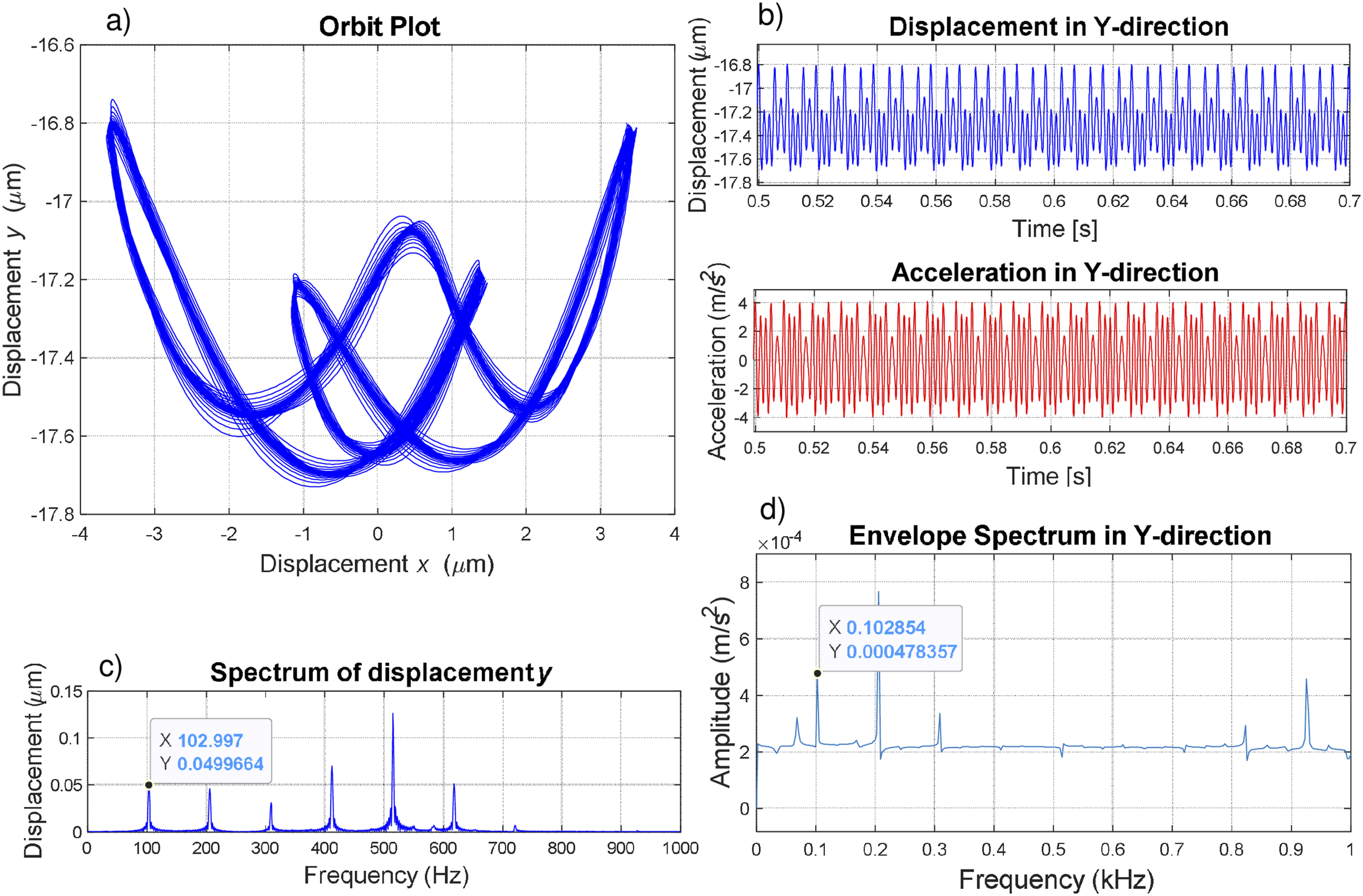

The orbit plot shows the position of the bearing inner race center, which initially displaces downward from its initial position due to radial load acting on the inner race and starts vibrating below it. As there is no external force acting along the X-axis, the inner race center does not displace in the horizontal direction, as in the case of vertical direction. Initially, the vibration of the inner race center is unstable, but after some time it reaches a steady state and vibrates in certain ranges. Therefore, in this study, initial vibrations for some duration (0 to 0.5 s) are neglected.

The displacement versus time waveform in the vertical direction shows the displacement of the inner race center, which takes place below its initial position as seen in the orbit plot. Since there is no defect, the peak-to-peak displacement in the Y-direction (PTPY) observed is 0.99 μm only (i.e., between −17.73 μm to −16.74 μm). Similarly, peak-to-peak acceleration in Y-direction (PTPAY) is 9.415 m/s² (i.e., between −4.592 to −4.823 m/s²).

In the frequency and envelope spectrums in the vertical direction, the dominant peaks are related to varying compliance vibrations, which rise due to the entry of each ball in the load zone at cage rotational frequency f_c. The varying compliance frequency is given by³⁶

VCF = f_{c} \times Z

(22)

where

f_{c} = (f_{s} / 2) (1 - D_{b} / D_{c})

and Z is the number of balls. The calculated varying compliance frequency from equation (22) is 102.99 Hz ∼ 103 Hz. In the envelope spectrum of normal bearing, the peaks are found at 102.99 Hz (1VC) and its harmonics, which corresponds to VCF and its harmonics. Similar results were observed by the researchers^{12,14–16,21,23,26} in their studies. They also observed the peaks at varying compliance frequencies for normal bearings. This validates the model developed for normal bearing in this study. The peaks found in each spectrum are of lower amplitudes.

Vibration responses of DGBB with localized ORD by using two defect functions

When a ball comes in contact with the localized ORD, the contact force on the contacting surfaces changes suddenly, which causes impact vibration. The frequency of impulses due to balls travelling over an ORD can be calculated by

Outer Race Defect Frequency (ORDF) = \frac{Z f_{s}}{2} (1 - \frac{D_{b}}{D_{c}})

(23)

For the selected speed of 2400 r/min, the ORDF calculated from equation (23) is 102.99 Hz. The value of ORDF for the defective bearing is the same as the value of VCF for the normal bearing due to the kinematic relationship. However, the amplitude of the peak at ORDF is much higher than that of VCF.²³

Here, the rectangular function and the half-sine wave function are used separately for modeling the ORD, i.e., for modeling the ball center path when the ball travels over the outer race defect zone, and then their vibration responses are compared with responses of normal bearing. The bearing parameters and the procedure of modeling of bearing with an ORD using these two functions are given in Section 2.

For the comparison purpose, a bearing with a defect length (L_d) of 0.5 mm and a defect depth (D_d) of 0.1 mm is used for both defect functions. For these values of defect sizes, the value of D_max calculated from equation (5) is 0.0043 mm.

Vibration responses of bearing with ORD modeled using a rectangular function

Figure 7 shows the orbit plot, time waveforms, frequency spectrum and envelope spectrum of the defective bearing modeled with a rectangular defect function. The orbit plot of the defective bearing shows a larger range of displacements of the inner race center in both X and Y directions than the normal bearing.

Figure 7.

Vibration responses of defective bearing running at 2400 r/min using rectangular defect function: (a) orbit plot, (b) time waveforms, (c) frequency spectrum and (d) envelope spectrum.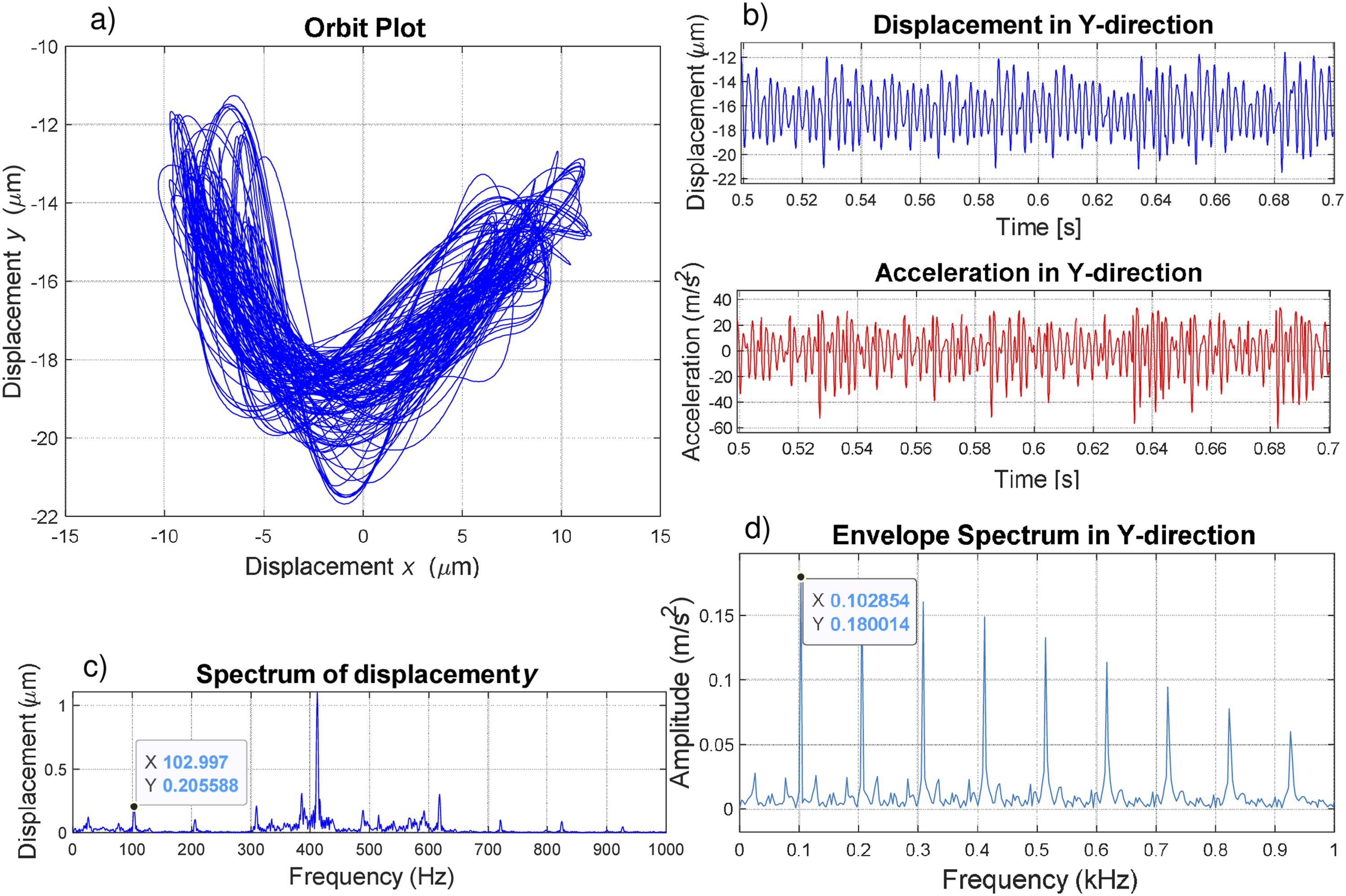

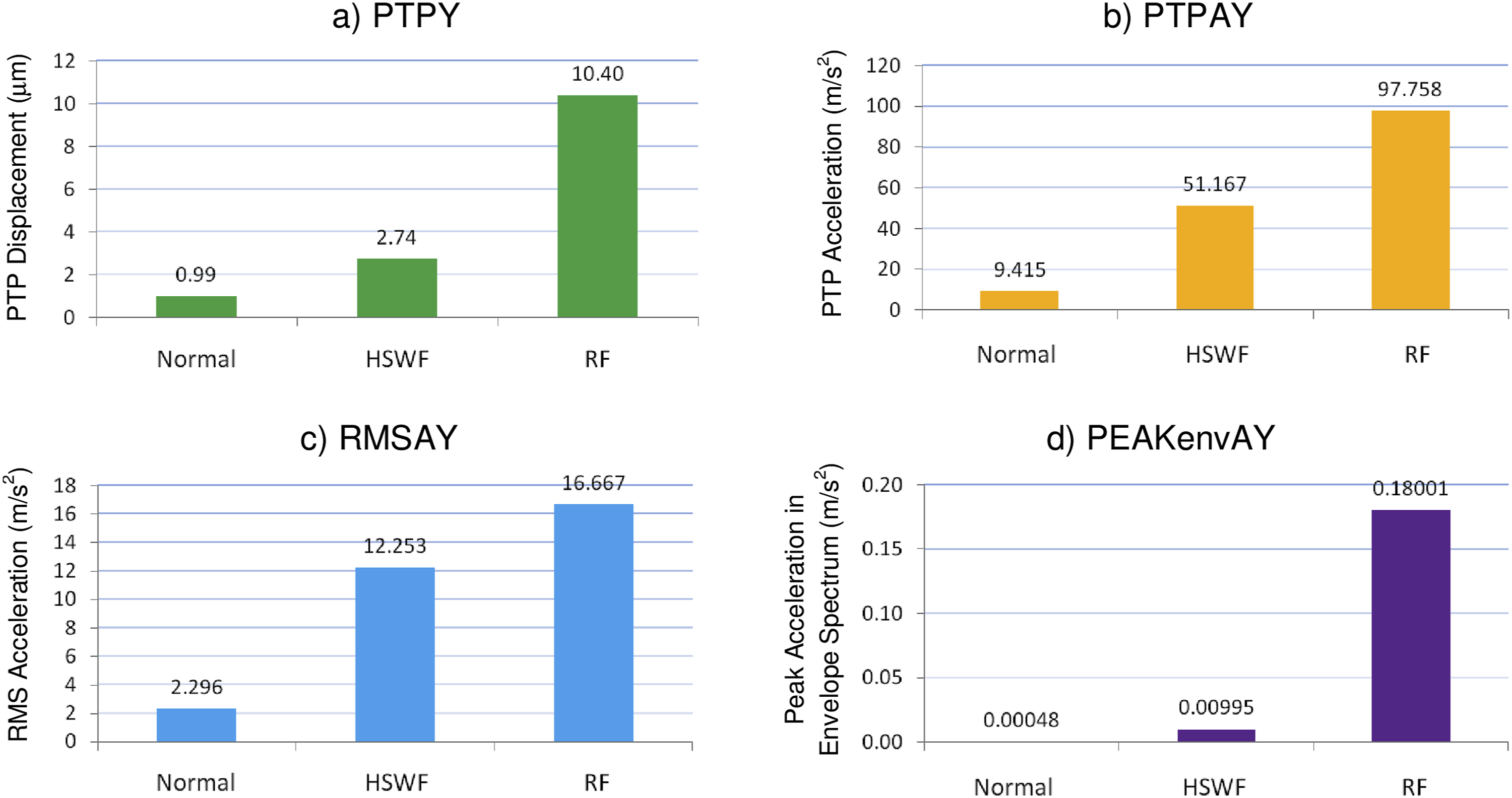
From the orbit plot and the displacement versus time waveform, it is observed that due to the ORD, the peak-to-peak displacement in Y-direction (PTPY) is increased to 10.40 μm (between −21.68 μm to −11.28 μm). Similarly, peak-to-peak acceleration in Y-direction (PTPAY) is increased to 97.758 m/s² (between −63.858 to +33.9 m/s²). These values are much higher than that of the normal bearing.

In both the frequency spectrum of displacement and envelope spectrum in the vertical direction, it is observed that the dominant peaks are related to ORDF, which rise due to the impact of the ball in the defect and due to abrupt changes in the ball center path in a rectangular shape. The peak amplitudes at ORDF found in the frequency spectrum of displacement and envelope spectrum in the vertical direction are 0.2055 μm and 0.18 m/s², which are much higher than the amplitudes at varying compliance frequency VCF of the normal bearing (0.0499 μm and 0.000478 m/s²).

Vibration responses of bearing with ORD modeled using a half-sine wave function

Figure 8 shows the orbit plot, time waveforms, frequency spectrum and envelope spectrum of the defective bearing modeled with a half-sine wave defect function. The orbit plot displays a larger range of displacements of the inner race centre in both X and Y directions than the normal bearing, but it shows a smaller range of displacements than a bearing modeled with a rectangular function.

Figure 8.

Vibration responses of defective bearing running at 2400 r/min using half-sine wave defect function: (a) orbit plot, (b) time waveforms, (c) frequency spectrum and (d) envelope spectrum.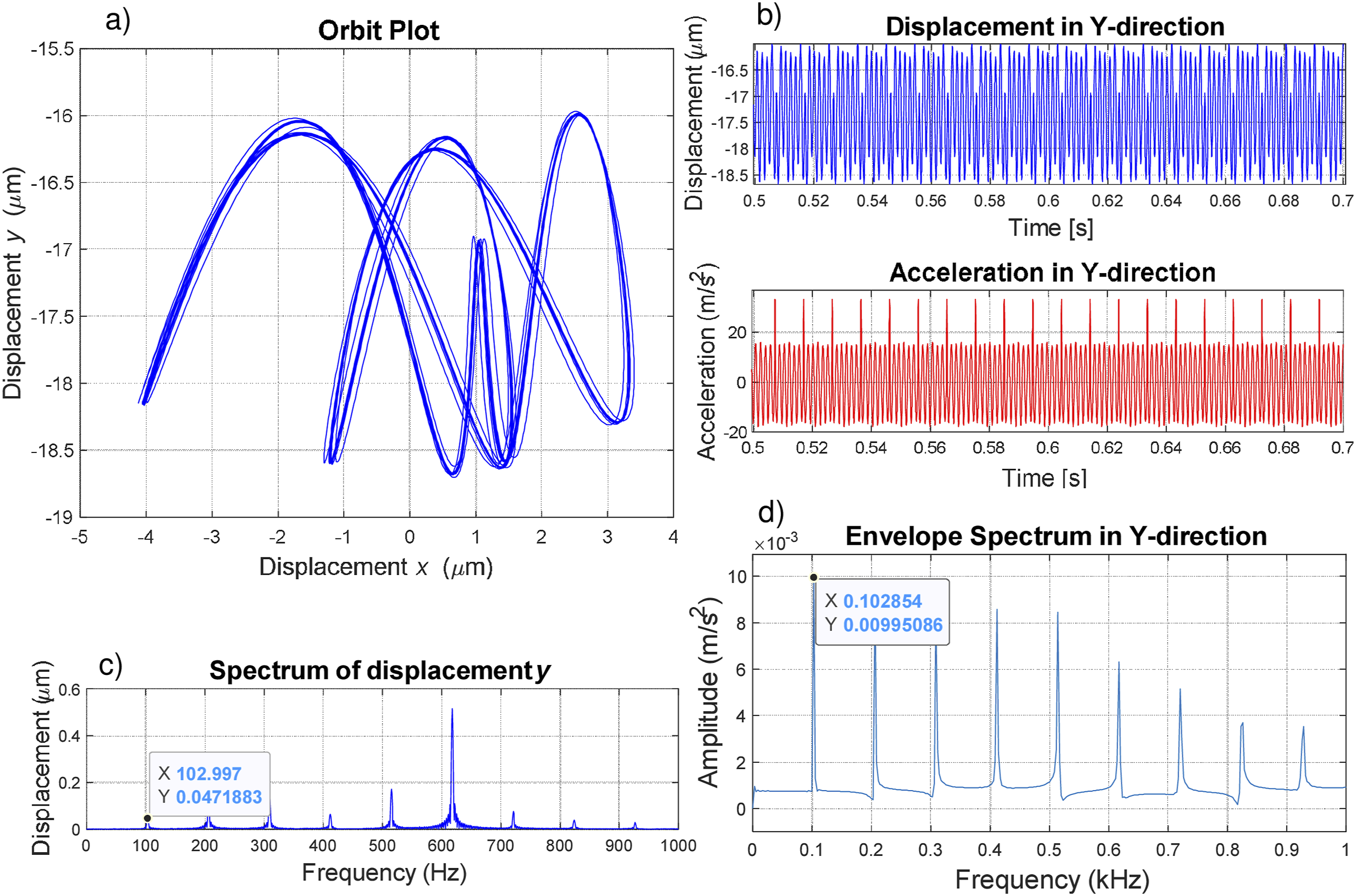

By observing the orbit plot and displacement versus time waveform, it is clear that due to the ORD, the peak-to-peak displacement in Y-direction (PTPY) is increased to 2.74 μm (i.e., between −18.7 μm to −15.96 μm), which is much higher than that for normal bearing (0.99 μm), but much lower than that of bearing modeled with a rectangular function (10.40 μm). Similarly, peak-to-peak acceleration in Y-direction (PTPAY) is increased to 51.167 m/s² (i.e., between −17.959 to +33.208 m/s²). These values are higher than that for normal bearing (9.415 m/s²) but much lower than that of bearing with rectangular defect function (97.758 m/s²).

In both the frequency spectrum of displacement and envelope spectrum in the vertical direction, the peaks at ORDF are found of 0.04718 μm and 0.00995 m/s² amplitude, respectively, which are much smaller than amplitudes of bearing with rectangular defect function (0.2055 μm and 0.18 m/s²).

The vibration responses of defective bearing modeled with a half-sine wave defect function look stable, unlike bearing with a rectangular defect function. This is due to the gradual radial displacement of the balls along the smooth curve generated by the sine wave function. It is observed from the envelope spectrums of the normal and defective bearings that the value of ORDF obtained for the defective bearing (102.854 Hz) is equal to the value of VCF obtained for the normal bearing. However, the amplitude of the peak at ORDF is much higher than that at VCF, which is also observed by many researchers.^{12,14–16,21,23,26} For the normal bearing, the amplitude of the peak at VCF observed is 0.000478 m/s² and for the defective bearing having a defect length of 0.5 mm, the amplitude of peak at ORDF is much higher. These amplitudes are 0.18 m/s² for the rectangular function and 0.00995 m/s² for the half-sine wave function.

Comparison of vibration responses obtained for normal bearing and defective bearings using two defect functions

Table 3 shows the vibration responses, i.e., peak-to-peak displacement in Y-direction (PTPY), peak-to-peak acceleration in Y-direction (PTPAY), RMS acceleration in Y-direction (RMSAY) and peak amplitude of acceleration in envelope spectrum in Y-direction (PEAKenvY) for normal and defective bearings. For defective bearings, vibration responses are shown for both the rectangular and half-sine wave functions. Figure 9 shows these responses in the graphical forms.

Table 3.

Vibration responses in Y-directions for normal and defective bearings.

Vibration response → Model of bearing ↓	PTPY (in μm)	PTPAY (in m/s²)	RMSAY (in m/s²)	PEAKenvY (in m/s²)
Defective bearing with RF	10.40	97.758	16.667	0.180014
Defective bearing with HSWF	2.74	51.167	12.253	0.009950
Normal bearing	0.99	9.415	2.296	0.000478

Figure 9.

Vibration responses in Y-directions for normal bearing and defective bearings with half-sine wave function and rectangular function.

Figure 9 and Table 3 clearly show that impulses of higher amplitude are generated when the bearing is modeled with a rectangular defect function. Therefore, it can be concluded that when a rectangular function is used for modeling the bearing defect, the peak amplitudes and overall vibrations are higher than the half-sine wave function. Higher values of vibration responses for defective bearings clearly indicate the presence of defect in the bearing.

Figure 10(a) and (b) show the displacement and acceleration, respectively, of the inner race center in the vertical direction for a short duration, obtained for the normal bearing and the defective bearing, whose ORD is modeled by using two defect functions.

Figure 10.

Comparison of vibration responses of bearing modeled with two defect functions.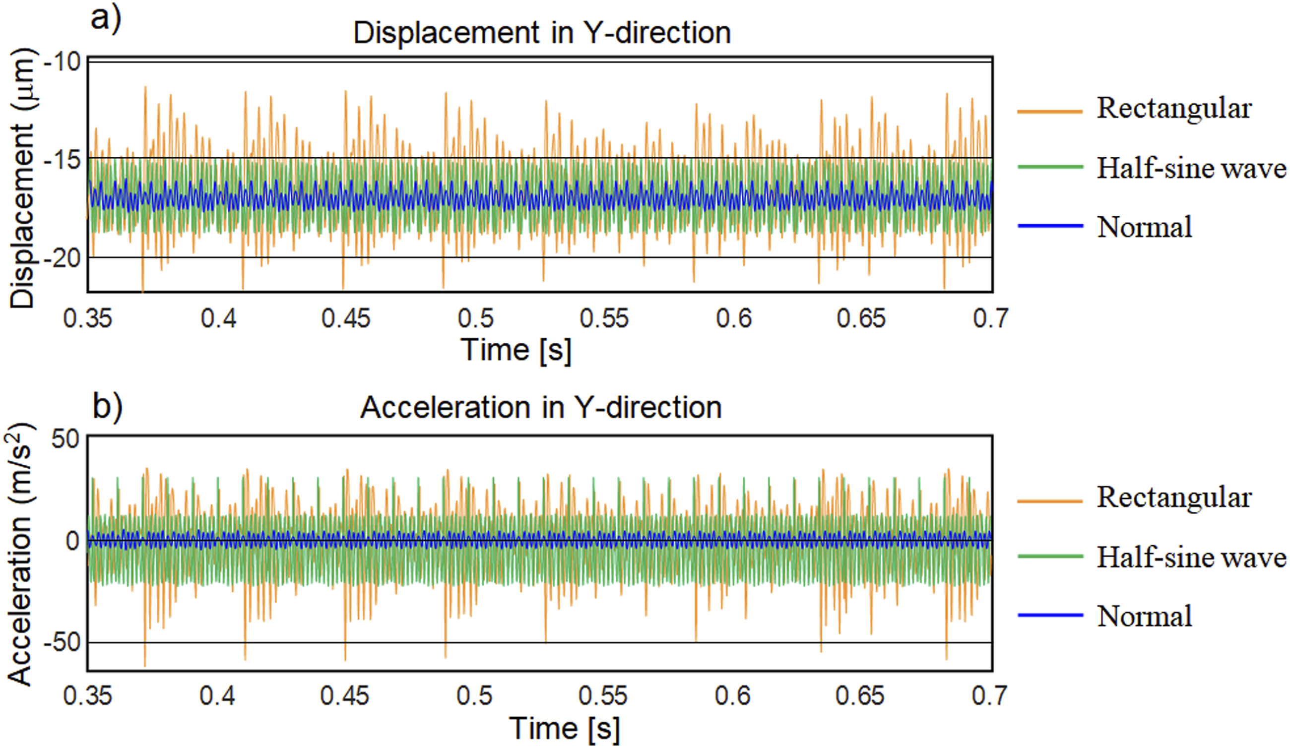

Effects of ORD length

In this section, the effects of the increase in defect length on the vibration responses of the bearing system are analyzed. The defect lengths used in the model are 0.05, 0.25, 0.5, 1, 1.5, 2 and 2.3 mm, and the defect depth is 0.1 mm. The values of D_max obtained for the selected defect lengths are shown in Table 2. Since D_max < D_d, the balls will not make contact with the bottom of the defect. The shaft speed used is 2400 r/min. Other bearing system specifications and the steps used for modeling and simulation are given in Section 2.

Two defect functions, i.e., a rectangular function and a half-sine wave function, are used separately for obtaining the vibration responses of the defective bearing having different defect lengths. Figures 11 and 12 show the vibration responses (envelope spectrums in the vertical direction) obtained for a defective bearing having different defect lengths by using both defect functions.

Figure 11.

Envelope spectrums of defective bearing with different defect lengths using rectangular defect function.

Figure 12.

Envelope spectrums of defective bearing with different defect lengths using half-sine wave defect function.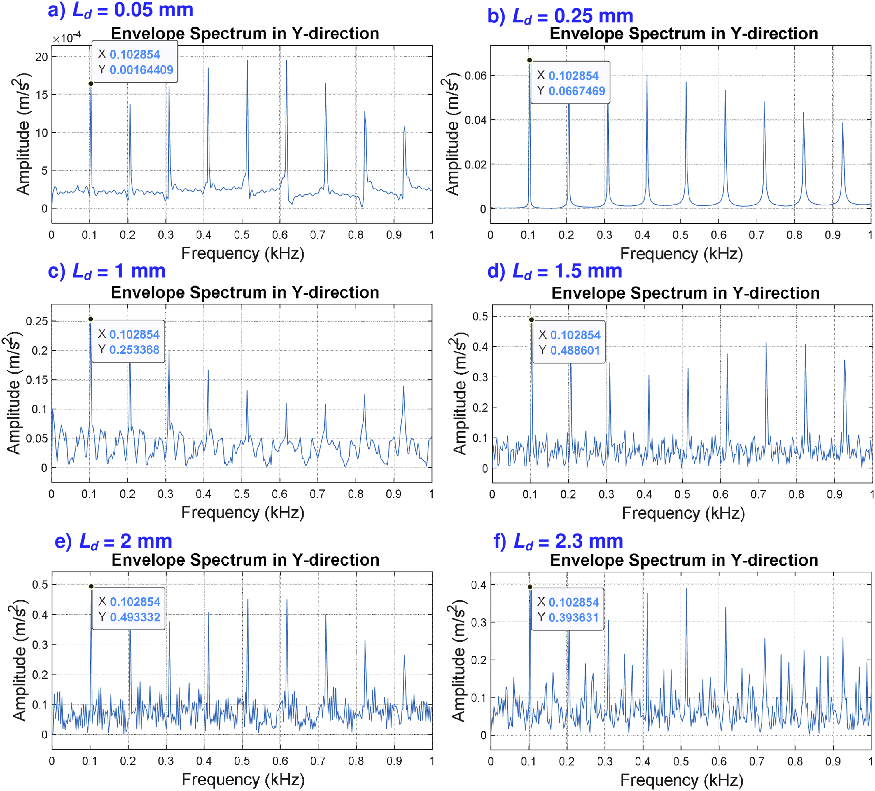

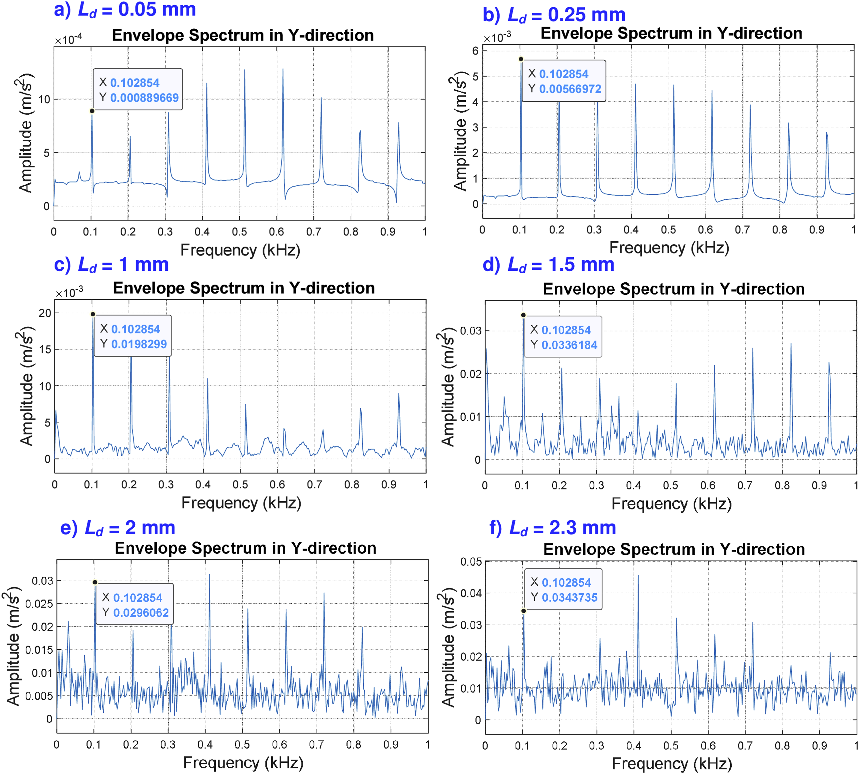
Figures 11 and 12 show that for each defect length, peaks are found at ORDF (102.85 Hz) and its harmonics and the vibration amplitudes for bearing modeled with a rectangular defect function are higher than modeled with a half-sine wave defect function. In addition, when the defect is at an incipient stage, i.e., when the defect length is small (0.05 to 0.25 mm), it is observed that the overall vibration is low and the peaks at the defect frequency are clearly seen. When the defect length increases (0.25 to 1 mm), the peak amplitude value increases quickly, while the overall vibration level (which is usually calculated using the RMS value) increases slowly. This increases the crest factor (i.e., Peak value/RMS value). However, when the defect length increases further (1 to 1.5 mm), the peak amplitude value does not increase, but the overall vibration level (RMS value) of the bearing system increases, which reduces the crest factor. Similar observations about peak, RMS and crest factor were also mentioned by the researchers earlier.^37–39 It is observed that when the defect length increases further (1.5 to 2.3 mm), the peak amplitude value decreases and the peaks at the defect frequency not seen clearly due to rise of peaks at sideband frequencies, which causes decrease in PTPAY, RMSAY and PEAKenvAY.

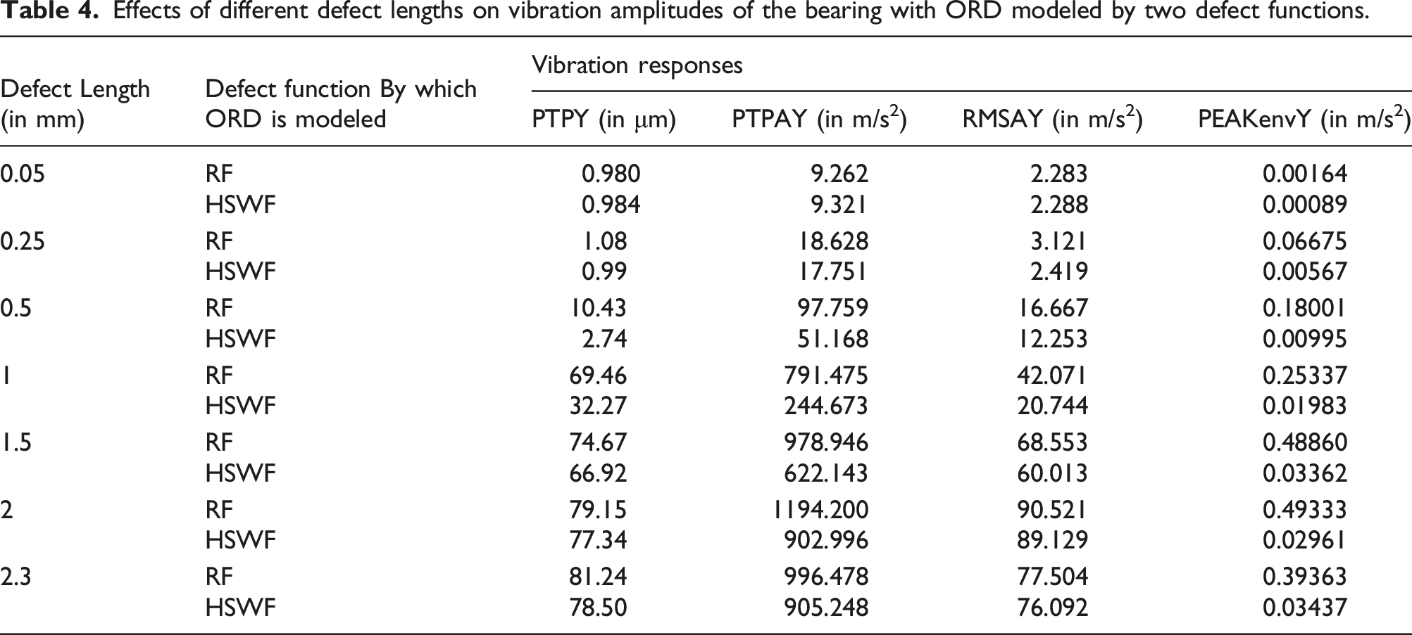
Table 4 and Figure 13 show effects of change in defect length on different vibration responses for the ball bearing having an ORD modeled by using two defect functions, separately, at a constant defect depth of 0.1 mm.

Table 4.

Effects of different defect lengths on vibration amplitudes of the bearing with ORD modeled by two defect functions.

Defect Length (in mm)	Defect function By which ORD is modeled	Vibration responses
Defect Length (in mm)	Defect function By which ORD is modeled	PTPY (in μm)	PTPAY (in m/s²)	RMSAY (in m/s²)	PEAKenvY (in m/s²)
0.05	RF	0.980	9.262	2.283	0.00164
0.05	HSWF	0.984	9.321	2.288	0.00089
0.25	RF	1.08	18.628	3.121	0.06675
0.25	HSWF	0.99	17.751	2.419	0.00567
0.5	RF	10.43	97.759	16.667	0.18001
0.5	HSWF	2.74	51.168	12.253	0.00995
1	RF	69.46	791.475	42.071	0.25337
1	HSWF	32.27	244.673	20.744	0.01983
1.5	RF	74.67	978.946	68.553	0.48860
1.5	HSWF	66.92	622.143	60.013	0.03362
2	RF	79.15	1194.200	90.521	0.49333
2	HSWF	77.34	902.996	89.129	0.02961
2.3	RF	81.24	996.478	77.504	0.39363
2.3	HSWF	78.50	905.248	76.092	0.03437

Figure 13.

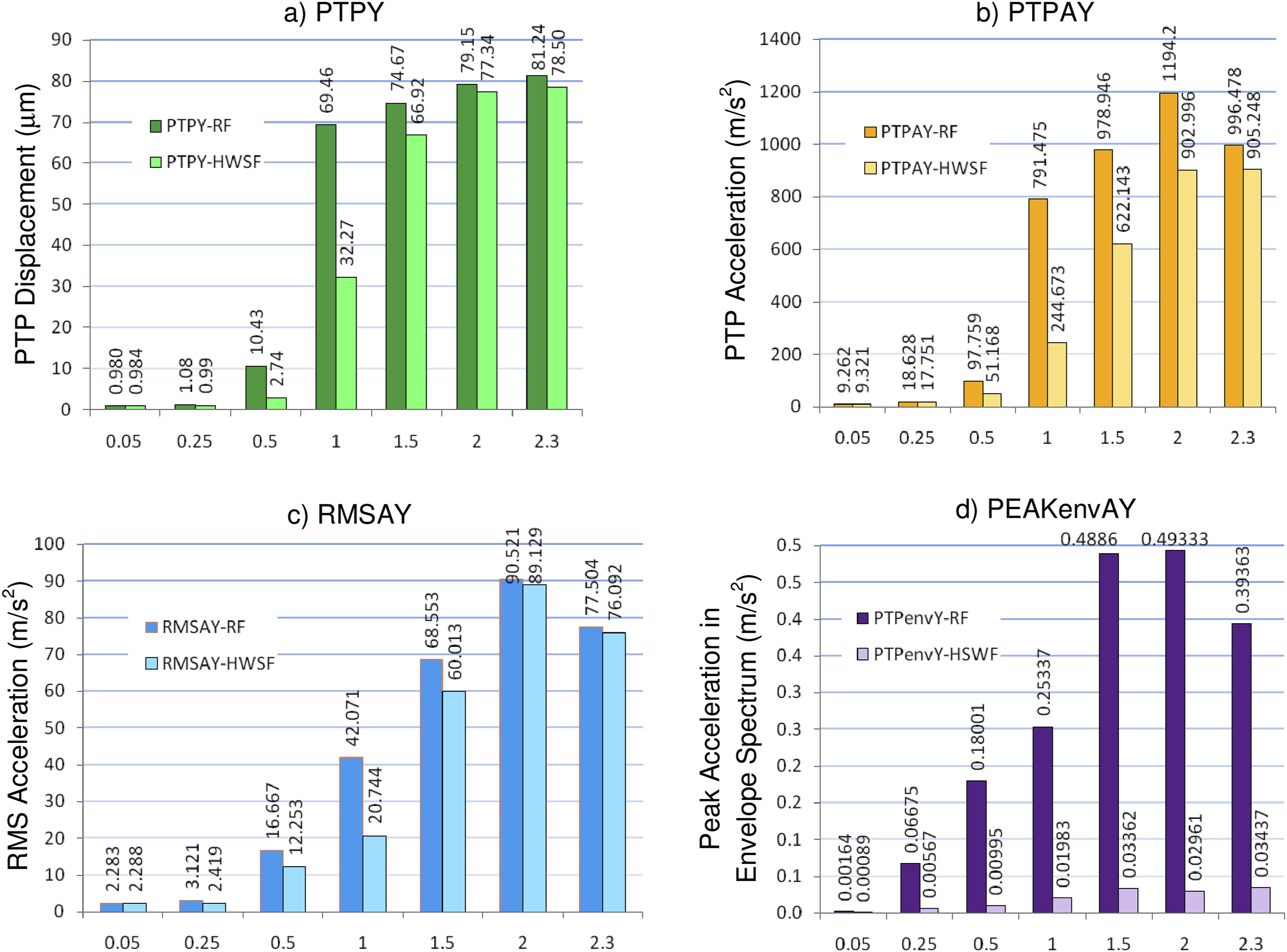
Effects of different defect lengths on different vibration responses for the bearing with ORD modeled by two defect functions.

From Table 4 and Figure 13, it is seen that for different defect lengths, the vibration responses for the bearing modeled with rectangular defect function are higher than that of the bearing modeled with half-sine wave function. Also, observed that with the increase in defect length, initially, the values of PTPAY, RMSAY and PEAKenvAY increase. However, after a certain defect length (here 2 mm), these values start decreasing.

Validation of the model

The validation of the model used in this study occurs at various stages of the paper, for example, in the envelope spectrum of the normal bearing, the peaks observed at 102.99 Hz, and its multiples, correspond to the VCF and its harmonics. Researchers^{12,14–16,21,23,26} have observed similar results in their studies. They also found peaks at varying compliance frequencies and their harmonics for normal bearings. Thus, the model used for the normal bearing can be considered valid. Similarly, for the bearing with ORD, the peaks are found at 102.85 Hz and its multiples, corresponding to the outer race defect frequency (ORDF) and its harmonics. Across all the models developed by researchers for ORD, the same findings are reported. The numerically calculated values of VCF and ORDF and their values obtained from the model match very well.

Moreover, the same model is used with the bearing specifications provided by Patil et al.¹³ using the half-sine wave defect function. Here, a defect length of 0.05 mm is selected, and the total defect depth of 0.1 mm is used for the time-varying radial displacement of the ball into the defect (Δ_d) as used by Patil et al. Figure 14(a) and (b) show the time waveform obtained by Patil et al. and by using the model used in this paper, respectively. The results correlate very well. The difference between two consecutive peaks (0.56643 – 0.487383 = 0.01926 s) corresponds to the ORDF (1/0.01926 = 51.92 Hz). This validates the model used for the defective bearings in this study.

Figure 14.

Time waveform obtained (a) by Patil et al.¹³ and (b) by the model in this study.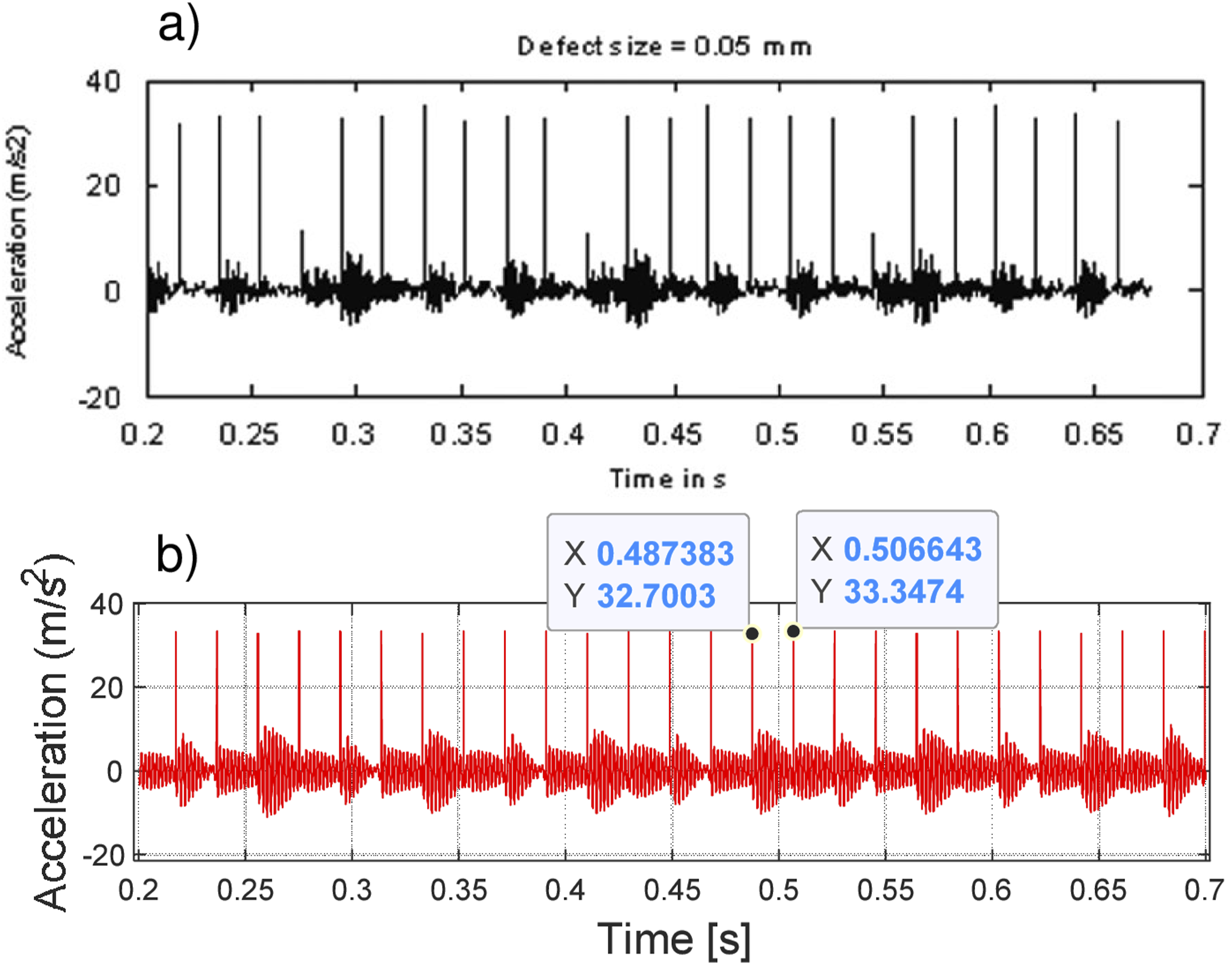

Conclusions

In this paper, a 2-DOF non-linear mathematical model of SKF 6305 DGBB with an outer race defect is developed using two defect functions, a rectangular function, and a half-sine wave function, and their vibration responses are compared. Also, the effects of increase in ORD length on bearing vibration responses are simulated and analyzed for two defect functions. Vibration responses obtained are in the vertical direction, which are peak-to-peak displacement, peak-to-peak acceleration, RMS acceleration and peak amplitude of acceleration in the envelope spectrum. The model is based on Hertzian contact deformation theory. In this model, a novel method, based on the analytical and graphical calculations is applied to find the maximum possible radial displacement of the ball into the defect. This displacement depends on race-ball-defect geometry and is obtained from the defect length, the radius of the ball, and the radius of the outer race. Based on the simulated results, the conclusions drawn are as follows.

• When the defect length is small, the vibration responses increase rapidly with the increase in defect length and when the defect length becomes large, the vibration responses start decreasing. This is because an increase in defect length leads to an increase in peaks at sideband frequencies and a decrease in peaks at defect frequencies.

• The vibration responses are higher when defects on the bearing are modeled using a rectangular defect function compared to modeling with a half-sine wave defect function. This is due to the generation of impacts caused by the abrupt changes in the ball center path within a rectangular shape, unlike the smooth curve of the sine wave.

• The functions used for modeling the defects are approximate functions that are based on certain assumptions. The vibration responses obtained using the rectangular function are higher than those obtained using the half-sine wave function, although their trends are similar with respect to an increase in defect length. Moreover, both functions reliably predict the presence of a defect in the bearing. A more realistic defect function can be modeled by considering the actual path of balls in defects.

• For the normal bearing, peaks occur at VCF and its harmonics, while for a bearing with an ORD, the peaks are found at ORDF and its harmonics. In both cases, these frequencies are identical. However, the vibration amplitude of ORDF is significantly higher than that of VCF.

The detailed comparison of two defect functions, along with their use in simulation and analysis of bearing system vibration, provides a sound base for researchers in the development of better realistic models. Also, the changes in the shapes of various plots and the different vibration responses due to the increase in defect length provide helpful simulated support to the vibration analyzers to understand the effects of the severity of the defects.

Footnotes

Declaration of conflicting interests

The author(s) declared no potential conflicts of interest with respect to the research, authorship, and/or publication of this article.

Funding

The author(s) received no financial support for the research, authorship, and/or publication of this article.

ORCID iD

Prashant H Jain

Appendix

The summary of latest literature on 2-DOF modeling of DGBBs with localized defects is given in Table 5. Table 5.

Summary of latest literature on 2-DOF modeling of DGBBs with localized defects.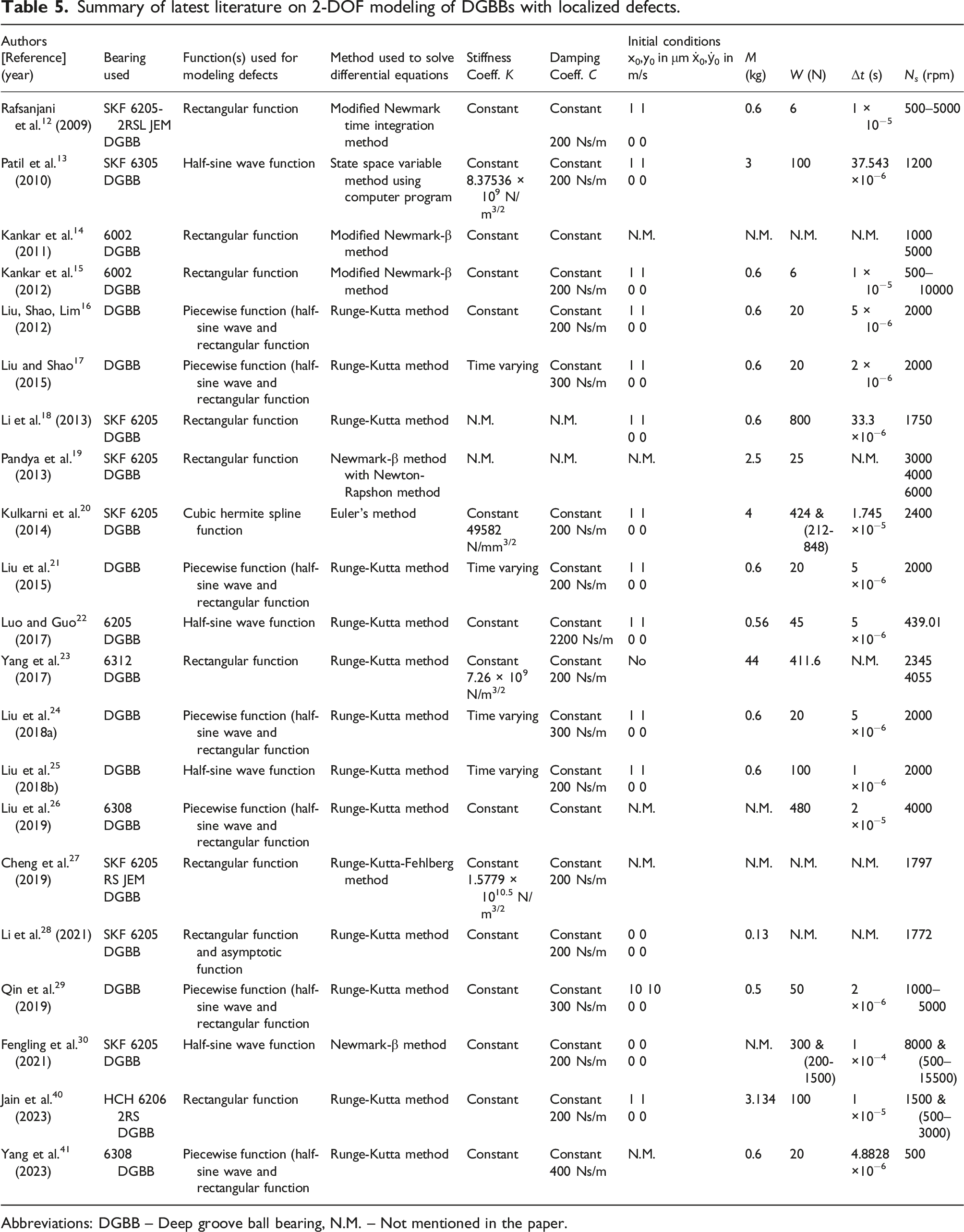

Authors [Reference] (year)	Bearing used	Function(s) used for modeling defects	Method used to solve differential equations	Stiffness Coeff. K	Damping Coeff. C	Initial conditions x₀,y₀ in μm ẋ₀,ẏ₀ in m/s	M (kg)	W (N)	Δt (s)	N_s (rpm)
Rafsanjani et al.¹² (2009)	SKF 6205-2RSL JEM	Rectangular function	Modified Newmark time integration method	Constant	Constant	1 1	0.6	6	1 × 10⁻⁵	500–5000
Rafsanjani et al.¹² (2009)	DGBB	Rectangular function	Modified Newmark time integration method	Constant	200 Ns/m	0 0	0.6	6	1 × 10⁻⁵	500–5000
Patil et al.¹³ (2010)	SKF 6305	Half-sine wave function	State space variable method using computer program	Constant	Constant	1 1	3	100	37.543	1200
Patil et al.¹³ (2010)	DGBB	Half-sine wave function	State space variable method using computer program	8.37536 × 10⁹ N/m^3/2	200 Ns/m	0 0	3	100	×10⁻⁶	1200
Kankar et al.¹⁴ (2011)	6002	Rectangular function	Modified Newmark-β method	Constant	Constant	N.M.	N.M.	N.M.	N.M.	1000
Kankar et al.¹⁴ (2011)	DGBB	Rectangular function	Modified Newmark-β method	Constant	Constant	N.M.	N.M.	N.M.	N.M.	5000
Kankar et al.¹⁵ (2012)	6002	Rectangular function	Modified Newmark-β method	Constant	Constant	1 1	0.6	6	1 × 10⁻⁵	500–10000
Kankar et al.¹⁵ (2012)	DGBB	Rectangular function	Modified Newmark-β method	Constant	200 Ns/m	0 0	0.6	6	1 × 10⁻⁵	500–10000
Liu, Shao, Lim¹⁶ (2012)	DGBB	Piecewise function (half-sine wave and rectangular function	Runge-Kutta method	Constant	Constant	1 1	0.6	20	5 × 10⁻⁶	2000
Liu, Shao, Lim¹⁶ (2012)	DGBB	Piecewise function (half-sine wave and rectangular function	Runge-Kutta method	Constant	200 Ns/m	0 0	0.6	20	5 × 10⁻⁶	2000
Liu and Shao¹⁷ (2015)	DGBB	Piecewise function (half-sine wave and rectangular function	Runge-Kutta method	Time varying	Constant	1 1	0.6	20	2 × 10⁻⁶	2000
Liu and Shao¹⁷ (2015)	DGBB	Piecewise function (half-sine wave and rectangular function	Runge-Kutta method	Time varying	300 Ns/m	0 0	0.6	20	2 × 10⁻⁶	2000
Li et al.¹⁸ (2013)	SKF 6205	Rectangular function	Runge-Kutta method	N.M.	N.M.	1 1	0.6	800	33.3	1750
Li et al.¹⁸ (2013)	DGBB	Rectangular function	Runge-Kutta method	N.M.	N.M.	0 0	0.6	800	×10⁻⁶	1750
Pandya et al.¹⁹ (2013)	SKF 6205	Rectangular function	Newmark-β method with Newton-Rapshon method	N.M.	N.M.	N.M.	2.5	25	N.M.	3000
	DGBB									4000
	DGBB									6000
Kulkarni et al.²⁰ (2014)	SKF 6205	Cubic hermite spline function	Euler’s method	Constant	Constant	1 1	4	424 & (212-848)	1.745	2400
	DGBB			49582	200 Ns/m	0 0			×10⁻⁵
	DGBB			N/mm^3/2	200 Ns/m	0 0			×10⁻⁵
Liu et al.²¹ (2015)	DGBB	Piecewise function (half-sine wave and rectangular function	Runge-Kutta method	Time varying	Constant	1 1	0.6	20	5	2000
Liu et al.²¹ (2015)	DGBB	Piecewise function (half-sine wave and rectangular function	Runge-Kutta method	Time varying	200 Ns/m	0 0	0.6	20	×10⁻⁶	2000
Luo and Guo²² (2017)	6205	Half-sine wave function	Runge-Kutta method	Constant	Constant	1 1	0.56	45	5	439.01
Luo and Guo²² (2017)	DGBB	Half-sine wave function	Runge-Kutta method	Constant	2200 Ns/m	0 0	0.56	45	×10⁻⁶	439.01
Yang et al.²³ (2017)	6312	Rectangular function	Runge-Kutta method	Constant	Constant	No	44	411.6	N.M.	2345
	DGBB			7.26 × 10⁹	200 Ns/m					4055
	DGBB			N/m^3/2						4055
Liu et al.²⁴ (2018a)	DGBB	Piecewise function (half-sine wave and rectangular function	Runge-Kutta method	Time varying	Constant	1 1	0.6	20	5	2000
Liu et al.²⁴ (2018a)	DGBB	Piecewise function (half-sine wave and rectangular function	Runge-Kutta method	Time varying	300 Ns/m	0 0	0.6	20	×10⁻⁶	2000
Liu et al.²⁵ (2018b)	DGBB	Half-sine wave function	Runge-Kutta method	Time varying	Constant	1 1	0.6	100	1	2000
Liu et al.²⁵ (2018b)	DGBB	Half-sine wave function	Runge-Kutta method	Time varying	200 Ns/m	0 0	0.6	100	×10⁻⁶	2000
Liu et al.²⁶ (2019)	6308	Piecewise function (half-sine wave and rectangular function	Runge-Kutta method	Constant	Constant	N.M.	N.M.	480	2	4000
Liu et al.²⁶ (2019)	DGBB	Piecewise function (half-sine wave and rectangular function	Runge-Kutta method	Constant	Constant	N.M.	N.M.	480	×10⁻⁵	4000
Cheng et al.²⁷ (2019)	SKF 6205	Rectangular function	Runge-Kutta-Fehlberg method	Constant	Constant	N.M.	N.M.	N.M.	N.M.	1797
	RS JEM			1.5779 × 10^10.5 N/m^3/2	200 Ns/m
	DGBB			1.5779 × 10^10.5 N/m^3/2	200 Ns/m
Li et al.²⁸ (2021)	SKF 6205	Rectangular function and asymptotic function	Runge-Kutta method	Constant	Constant	0 0	0.13	N.M.	N.M.	1772
Li et al.²⁸ (2021)	DGBB	Rectangular function and asymptotic function	Runge-Kutta method	Constant	200 Ns/m	0 0	0.13	N.M.	N.M.	1772
Qin et al.²⁹ (2019)	DGBB	Piecewise function (half-sine wave and rectangular function	Runge-Kutta method	Constant	Constant	10 10	0.5	50	2	1000–5000
Qin et al.²⁹ (2019)	DGBB	Piecewise function (half-sine wave and rectangular function	Runge-Kutta method	Constant	300 Ns/m	0 0	0.5	50	×10⁻⁶	1000–5000
Fengling et al.³⁰ (2021)	SKF 6205	Half-sine wave function	Newmark-β method	Constant	Constant	0 0	N.M.	300 & (200-1500)	1	8000 & (500–15500)
Fengling et al.³⁰ (2021)	DGBB	Half-sine wave function	Newmark-β method	Constant	200 Ns/m	0 0	N.M.	300 & (200-1500)	×10⁻⁴	8000 & (500–15500)
Jain et al.⁴⁰ (2023)	HCH 6206 2RS DGBB	Rectangular function	Runge-Kutta method	Constant	Constant	1 1	3.134	100	1	1500 & (500–3000)
Jain et al.⁴⁰ (2023)	HCH 6206 2RS DGBB	Rectangular function	Runge-Kutta method	Constant	200 Ns/m	0 0	3.134	100	×10⁻⁵	1500 & (500–3000)
Yang et al.⁴¹ (2023)	6308 DGBB	Piecewise function (half-sine wave and rectangular function	Runge-Kutta method	Constant	Constant	N.M.	0.6	20	4.8828	500
Yang et al.⁴¹ (2023)	6308 DGBB	Piecewise function (half-sine wave and rectangular function	Runge-Kutta method	Constant	400 Ns/m	N.M.	0.6	20	×10⁻⁶	500

Abbreviations: DGBB – Deep groove ball bearing, N.M. – Not mentioned in the paper.

References

Howard

. A review of rolling element bearing vibration “Detection, diagnosis and prognosis”. Melbourne, Victoria, Australia: Defence Science and Technology Organization, Aeronautical and Maritime Research Laboratory, 1994.

Jain

Bhosle

. A review on vibration signal analysis techniques used for detection of rolling element bearing defects. Int J Mech Eng 2021; 8: 14–29.

Liu

Shao

Zuo

. The effects of the shape of localized defect in ball bearings on the vibration waveform. Proc Inst Mech Eng - Part K J Multi-body Dyn 2013; 227: 261–274.

Jain

Bhosle

. Analysis of vibration signals caused by ball bearing defects using time-domain statistical indicators. IJATEE. 2022; 9: 700–715.

Singh

Howard

Hansen

. An extensive review of vibration modelling of rolling element bearings with localised and extended defects. J Sound Vib 2015; 357: 300–330.

El-Thalji

Jantunen

. A summary of fault modelling and predictive health monitoring of rolling element bearings. Mech Syst Signal Process 2015; 60–61: 252–272.

Khanam

Tandon

Dutt

. A review of vibration modeling of ba ll bearings with local defect . Visakhapatanm, India: Proceedings of International Conference on Condition Monitoring (ICCM2016), 26-27 October 2016, pp. 215–224.

Cao

Niu

, et al. Mechanical model development of rolling bearing-rotor systems: a review. Mech Syst Signal Process 2018; 102: 37–58.

Liu

Shao

. Overview of dynamic modelling and analysis of rolling element bearings with localized and distributed faults. Nonlinear Dyn. 2018; 93: 1765–1798.

10.

Sharma

Upadhyay

Kankar

, et al. Nonlinear dynamic investigations on rolling element bearings: a review. Adv Mech Eng. 2018; 10: 168781401876414.

11.

Kong

Huang

Jiang

, et al. A vibration model of ball bearings with a localized defect based on the hertzian contact stress distribution. Shock Vib 2018; 2018: 1–14.

12.

Rafsanjani

Abbasion

Farshidianfar

, et al. Nonlinear dynamic modeling of surface defects in rolling element bearing systems. J Sound Vib 2009; 319: 1150–1174.

13.

Patil

Mathew

Rajendrakumar

, et al. A theoretical model to predict the effect of localized defect on vibrations associated with ball bearing. Int J Mech Sci 2010; 52: 1193–1201.

14.

Kankar

Sharma

Harsha

. Fault diagnosis of high speed rolling element bearings due to localized defects using response surface method. J Dyn Syst Meas Control 2011; 133: 031007.

15.

Kankar

Sharma

Harsha

. Vibration based performance prediction of ball bearings caused by localized defects. Nonlinear Dyn 2012; 69: 847–875.

16.

Liu

Guan

, et al. Hemoglobin immobilized with modified “fish-in-net” approach for the catalytic removal of aniline. J Hazard Mater 2012; 217–218: 156–163.

17.

Liu

Shao

. A new dynamic model for vibration analysis of a ball bearing due to a localized surface defect considering edge topographies. Nonlinear Dyn 2015; 79: 1329–1351.

18.

Zhu

Zhou

, et al. Fault diagnosis based on nonlinear dynamic modeling in rolling element bearing systems. In: 2013 IEEE International Symposium on Assembly and Manufacturing (ISAM), Xi'an, China, 30 July 2013, pp. 12–15.

19.

Pandya

Upadhyay

Harsha

. Nonlinear dynamic analysis of high speed bearings due to combined localized defects. J Vib Control 2014; 20: 2300–2313.

20.

Kulkarni

Sahasrabudhe

. A dynamic model of ball bearing for simulating localized defects on outer race using cubic hermite spline. J Mech Sci Technol 2014; 28: 3433–3442.

21.

Liu

Shao

Zhu

. A new model for the relationship between vibration characteristics caused by the time-varying contact stiffness of a deep groove ball bearing and defect sizes. J Tribol 2015; 137: 031101.

22.

Luo

Guo

. Dynamic mechanism modeling for dual-impulse behavior excited by a spall on outer race of ball bearing. Vib proced 2017; 14: 57–63.

23.

Yang

Jin

Hou

, et al. Study for ball bearing outer race characteristic defect frequency based on nonlinear dynamics analysis. Nonlinear Dyn 2017; 90: 781–796.

24.

Liu

Shi

Shao

. A theoretical study for the influence of the combined defect on radial vibrations of a ball bearing. ILT 2018; 70: 339–346.

25.

Liu

Shao

. A theoretical study on vibrations of a ball bearing caused by a dent on the races. Eng Fail Anal 2018; 83: 220–229.

26.

Liu

, et al. An analytical method for dynamic analysis of a ball bearing with offset and bias local defects in the outer race. J Sound Vib 2019; 461: 114919.

27.

Cheng

Zhang

, et al. Research on ball bearing model based on local defects. SN Appl Sci 2019; 1: 1219.

28.

Tian

, et al. Dynamic asymptotic model of rolling bearings with a single fault in the inner raceway. Adv Mech Eng 2021; 13: 168781402110522.

29.

Qin

Cao

Wang

, et al. Dynamics modelling for deep groove ball bearings with local faults based on coupled and segmented displacement excitation. J Sound Vib 2019; 447: 1–19.

30.

Fengling

Yuwei

Jiaoyue

, et al. Fault dynamic modeling and characteristic parameter simulation of rolling bearing with inner ring local defects. Shock Vib 2021; 2021: 1–11.

31.

Jain

Bhosle

. Mathematical modeling, simulation and analysis of non-linear vibrations of a ball bearing due to radial clearance and number of balls. Mater Today Proc. 2023; 72: 927–936.

32.

Kumbhar

Sudhagar P

Desavale

. An overview of dynamic modeling of rolling-element bearings. Noise Vib Worldw 2021; 52: 3–18.

33.

Harris

. Rolling bearing analysis. Hoboken, NJ: John Wily and Son, INC., 2001.

34.

Jain

Bhosle

. Analysis of effects of radial clearance and unbalance on vibration responses of a rotor-bearing system. Int J Eng Trends Technol. 2022; 70: 327–347.

35.

Jain

Bhosle

Keche

Desavale

. Analysis of vibration of a rotor-bearing system caused by radial clearance, number of balls and rotor speed. Recent Advances in Mechanical Engineering, Volume 1. Singapore: Springer Nature, 2024, 1. https://link-springer-com-443.web.bisu.edu.cn/book/9789819709175, In press.

36.

Tiwari

Gupta

Prakash

. Effect of radial internal clearance of a ball bearing on the dynamics of a balanced horizontal rotor. J Sound Vib 2000; 238: 723–756.

37.

Sun

Krishnappa

. Bearing diagnostics based on pattern recognition of statistical parameters. J Vib Control 2000; 6: 375–392.

38.

Jain

Bhosle

. Study of effects of radial load on vibration of bearing using time-domain statistical parameters. IOP Conf Ser Mater Sci Eng 2021; 1070: 012130.

39.

Xiang

Zhu

. An engineering condition indicator for condition monitoring of wind turbine bearings. Wind Energy 2020; 23: 207–219.

40.

Jain

Bhosle

Keche

, et al. A dynamic model of outer race defective bearing considering the unbalanced shaft-bearing system with experimental simulation. ASME’s Journal of Tribology. 2024; 146(1): 014301.

41.

Yang

Sun

, et al. Analytical modeling and mechanism analysis of time-varying excitation for surface defects in rolling element bearings. J Dyna Monit Diag 2023; 2: 89–101.

Comparison of non-linear vibration of outer race defective ball bearing using two defect functions

Abstract

Keywords

Introduction

Modeling of DGBB with localized outer race defect

Bearing input parameters and assumptions

Calculation of contact deformation δ

Equivalent contact stiffness K between ball and races, and damping coefficient C of the inner race

Calculation of contact (restoring) forces between the balls and races

Formulation of differential equations of motion

Solution of differential equations of motion

Presentation of results

Results and discussion

Vibration responses of normal DGBB

Vibration responses of DGBB with localized ORD by using two defect functions

Vibration responses of bearing with ORD modeled using a rectangular function

Vibration responses of bearing with ORD modeled using a half-sine wave function

Comparison of vibration responses obtained for normal bearing and defective bearings using two defect functions

Effects of ORD length

Validation of the model

Conclusions

Footnotes

Declaration of conflicting interests

Funding

ORCID iD

Appendix

References

Calculation of contact deformation $δ$