Enhancing noise assessment accuracy: FEM as an advanced complement to CNOSSOS-EU

Abstract

This study explores the enhancement of noise assessment accuracy by integrating the Finite Element Method (FEM) as a complementary approach to the Common Noise Assessment Methods in Europe (CNOSSOS-EU). CNOSSOS-EU, widely adopted as the reference for strategic noise mapping across Europe and beyond, provides an semi-empirical model for noise propagation based on experimental algorithms and simplifications. While robust, CNOSSOS-EU’s approach can overlook the complex physical and geometric characteristics of certain environments, particularly in detailed or high-stakes noise assessments. To address these limitations, this work demonstrates how FEM—rooted in fundamental physical principles—can serve as a powerful adjunct to CNOSSOS-EU, offering finer detail in modeling noise propagation in complex environments. By comparing and validating FEM-derived results against those of CNOSSOS-EU, this study identifies key discrepancies and analyzes their implications for noise management strategies. The findings underscore the added value of integrating FEM, ultimately supporting more informed decision-making and the development of effective noise control measures.

Keywords

Noise Assessment CNOSSOS-EU finite element method (FEM)strategic noise mapping noise control strategies

Introduction

Human development, particularly that related to urban growth, the creation of transport infrastructures and economic and industrial activity, has generated, among other adverse environmental effects, an increase in the exposure of the population to environmental noise. This has led to growing concern about noise impact on human and wildlife health.¹

Prolonged exposure to environmental noise is associated with a variety of adverse effects. These effects include stress, sleep disorders, cardiovascular disease, and others, which cause a decrease in quality of life.^2–6

In response to these threats, the European Union has adopted progressive policies to manage and mitigate environmental noise. The most relevant ones are those derived from Directive 2002/49/EC, known as the Environmental Noise Directive (END). This Directive establishes a common framework for tackling the noise problem in the Member States. It mandates assessing noise exposure using noise maps and developing action plans to reduce noise where necessary.

The END has also encouraged the development and adoption of simulation methods for the accurate assessment of environmental noise.

In this context, CNOSSOS-EU is presented as the standardized method recommended by the European Commission for the assessment (prediction) of environmental noise in European Member States. Its use is mandatory in the strategic noise mapping from major acoustic emitters.⁷

Unlike interim methods (non-standardized, although widely accepted, national methodologies), CNOSSOS-EU provides a coherent and harmonized approach to environmental noise assessment. It seeks to improve the comparability and reliability of noise data across Europe.

CNOSSOS-EU is a semi-empirical method based on experimental formulas and algorithms, or simplifications to estimate noise propagation. In contrast, the FEM methodology employs purely theoretical methods or those based on fundamental physical principles.

This paper focuses on the comparison and validation of the results obtained by FEM with those provided by CNOSSOS-EU, identifying discrepancies and analyzing the underlying causes.

Literature review

The application of the Finite Element Method (FEM) in environmental acoustics is an area of research that has gained relevance due to its ability to model complex environments and provide detailed information on noise propagation.^8–11

FEM is a numerical technique used to solve partial differential equations in complex domains,¹² applicable, among other areas, to the modeling of sound waves. Unlike semi-empirical methods, such as CNOSSOS-EU, FEM is based on fundamental physical principles, allowing for a detailed analysis of acoustic interactions in complex environments.^10,13

CNOSSOS-EU, on the other hand, is a method developed to standardize noise assessment in Europe. This method uses experimental formulas and algorithms to estimate noise propagation, providing a harmonized approach to environmental noise assessment.^7,14

However, despite its strengths, CNOSSOS-EU, like any model based on empirical approaches mainly, has limitations in accurately capturing the physical and geometric complexity of sound propagation in specific environments.^15–17

Studies with FEM have demonstrated their effectiveness in modeling noise propagation in environments where semi-empirical methods are not adequate.^18,19 For instance, Papadakis and Stavroulakis¹⁰ highlight that FEM provides an accurate estimate of the loss due to the insertion of acoustic barriers, overcoming the limitations of semi-empirical models. Marburg and Nolte¹³ underline the usefulness of FEM in the simulation of complex acoustic environments.

In addition to the FEM, other numerical methods such as the Finite Difference Method (FDM), the Finite Volume Method (FVM), and the Boundary Element Method (BEM) have established themselves as fundamental tools in the field of environmental and building acoustics. These methods offer an unprecedented ability to model sound propagation in complex environments, which can lead to better design and evaluation of noise correction and mitigation measures.^13,20,21

Despite its advantages, the application of FEM in environmental noise assessment presents challenges, including its high computational cost, high knowledge requirements in computational physics,²² and the need for detailed, hard-to-obtain input data. It is, therefore, necessary to establish in which situations the use of one or the other method is appropriate.

Given the need for precise technical studies for the assessment and correction of environmental noise, the present study aims to explore environmental noise assessment using FEM as a complementary tool to CNOSSOS-EU. This approach intends to overcome the limitations of empirical and semi-empirical methods by applying fundamental physical principles, seeking a more detailed assessment of environmental noise in complex environments. The ray-tracing method, as implemented in CNOSSOS-EU, is highly numerically efficient and well-suited for high-frequency sound propagation. In contrast, the FEM method becomes computationally expensive, particularly at high frequencies, regardless of whether a temporal or frequency-domain simulation is used, as the resolution of high-frequency components requires extremely small time-step sizes in temporal simulations.

Integrating FEM as a complementary tool to studies with CNOSSOS-EU could improve the accuracy of noise assessments by addressing its limitations. While CNOSSOS-EU provides an adequate overview for strategic noise mapping, it may not offer a detailed view of specific environments, considering complex interactions and environmental factors, and it is desirable to apply more accurate methods, for example, to model the insertion loss of noise barriers in complex environments, providing a more accurate representation of their performance in comparison with empirical and semi-empirical methods.

It should be noted that, although the application of computational physics to the assessment of environmental and underwater noise is the subject of several recent studies,^23,24 and that the application of the CNOSSOS-EU method is also the subject of numerous recent studies,^17,25–31 there are few studies³² that deal with both methodologies together, and none have been found that specifically combine the computational physics methods with the CNOSSOS-EU method, as it is done in the present study.

Objectives

The main aim of this work is to deepen the usefulness of advanced numerical simulation methods, in particular the Finite Element Method (FEM), combined with the CNOSSOS-EU method, to overcome the limitations in terms of accuracy in the modeling of ambient noise propagation.

In order to achieve this main aim, this study seeks to analyze in which aspects the implementation of FEM, as a complementary tool to CNOSSOS-EU, can help to better understand the physical and geometric complexities of the environment that CNOSSOS-EU simplify and, in this way, to improve the assessment of environmental noise.

In addition, it is intended to compare the results of both methodologies to identify discrepancies, as well as to help understand their cause, and the best interpretation of the two approaches.

Methods and data

Methodological approaches

In this work, two different approaches have been studied. On the one hand, methods based on the Wave Equation implemented with FEM, and within them both transient and stationary systems. On the other hand, the CNOSSOS-EU method that applies a combination of equations based on physics and experimental results, to estimate the propagation paths and the sound pressure level in the receiver.

The Wave Equation and Helmholtz Equation approaches, compared to empirical and semi-empirical methods, represent different methodologies for analyzing sound propagation in the acoustic scenario. These differences lie in the theoretical basis, the modeling approach, and the practical applications of each method.

The Wave Equation and Helmholtz Equation are based on the physical-mathematical analysis of the propagation of waves in the propagation medium.

The Wave Equation is used to model the propagation of sound waves in time and space, capturing the temporal dynamics of the waves.^33,34

The Helmholtz Equation, derived from the Wave Equation, focuses on the spatial distribution of sound pressure or sound field intensity at a specific frequency, being suitable for steady-state studies.^35,36

Unlike the previous ones, CNOSSOS-EU is based on the Ray Tracing technique^37,38 to calculate a hypothetical sound path. In this way, CNOSSOS-EU simplifies the study of propagation by tracing rays from sound sources. It analyses how these rays interact with the environment through reflections, refractions, and diffractions.

The ray tracing method is widely used in predicting sound propagation in outdoor and indoor environments, providing an effective tool for evaluating sound in complex spaces.³⁹ This method is also computationally much less demanding than the Finite Element Method.

Software tools used

In this work, two open-source software tools have been used. One for FEM simulations of the Wave and Helmholtz equations, known as Elmer FEM or just Elmer, and another for simulations with CNOSSOS-EU, known as Noise Modelling.

The Elmer FEM¹ software is used for the simulation of multi-physical processes, and it is based on the finite element method (FEM). It has been developed mainly by the CSC - IT Center for Science in Finland. It is designed to address complex simulations in fields such as fluid mechanics, heat transfer, electromagnetism, and acoustics, among others.⁴⁰

The version of Elmer FEM used was the February 7, 2024, build for Windows 64-bit, with graphical environment (ElmerGUI).²

The Noise Modelling software is designed to produce environmental noise maps of urban areas, roads, railways, and industrial sources. It can be used as a Java library or controlled through a Web interface.

The Noise Modelling project is led by acousticians from the Joint Research Unit in Environmental Acoustics (UMRAE, Gustave Eiffel University – CEREMA, France) and specialists in Geographic Information Sciences from the Lab-STICC laboratory (CNRS – DECIDE Team, France).³ As stated on its official Web site,⁴ it can be used freely for research, education or by experts in a professional use.

Noise Modelling has been used in different academic and institutional works. Among them, it is worth highlighting the French Government’s strategic road and railway noise maps, corresponding to the Fourth Round of the END. The periodic updating of these maps is possible on the basis of a national database (PlaMADE), which also feeds the Noise Modelling software.^41,42 The Noise Modelling version used for this study has been number 4.0.5, available on GitHub since September 2023.

Fundamentals of the wave equation and its formulation in Elmer FEM

Fundamentals of the wave equation

The Wave Equation describes how waves propagate through various media. It is applied to a wide range of phenomena, from sound waves and the simulation of waves in water, to the propagation of electromagnetic waves.

The three-dimensional generalization of the Wave equation (1) is expressed as:

\partial^{2} \frac{u}{\partial t^{2}} = c^{2} \nabla^{2} u

(1)

where u is the displacement of the wave at time t, and c is the velocity of propagation of the wave in the medium. The Laplacian operator (∇) is defined as (equation (2)):

\nabla^{2} u = \partial^{2} \frac{u}{\partial x^{2}} + \partial^{2} \frac{u}{\partial y^{2}} + \partial^{2} \frac{u}{\partial z^{2}}

(2)

This move toward three-dimensional systems allows the modeling of wave propagation in more realistic environments, being widely used in disciplines such as seismic engineering, room acoustics and optics.⁴³ This derivation of the Wave Equation for sound waves is based on the combination of Newton’s laws with the equations of continuity and state for fluids.⁴⁴

The Wave Equation does not only apply to the fields described above. For example, the Klein-Gordon and Schrödinger equations are versions of the Wave Equation that incorporate the principles of quantum mechanics and special relativity.⁴⁵

The Elmer wave equation

Elmer implements a generalized version of the Wave Equation (equation (3)) in the time domain.⁴⁶

- \frac{1}{c^{2}} \frac{\partial^{2} p}{\partial t^{2}} + Δ p + \frac{η}{c^{2}} Δ (\frac{\partial p}{\partial t}) - \frac{α}{c^{2}} \frac{\partial p}{\partial t} = f

(3)

where f a source function, e.g. pressure.

The terms η and α are parameters of the model, which can be set to zero to obtain the standard Wave Equation:

• ∂²p/∂t²: is the second derivative of pressure, p, with respect to time, t. Describes how pressure acceleration behaves over time.

• Δp: represents the increment of pressure, describing the change in pressure between two consecutive points.

• η and α: These are parameters of the model that adjust the equation to account for additional effects such as viscosity and medium reaction:

○ η: Adjust the Wave Equation to account for the effects of the viscosity of the medium through which the wave propagates.

○ α: Adjust the Wave Equation to include medium reaction effects, such as sound absorption not directly related to viscosity.

• ∂p/∂t: Indicates how the pressure changes over time.

Elmer also allows to specify boundary conditions to effectively simulate how waves interact with the boundaries of the simulation geometry. This includes:

• Dirichlet conditions: Where fixed values of pressure are specified at the boundaries of the domain.

• Neumann conditions: Where the rates of pressure change at the boundaries are specified, useful for modeling the interaction of sound waves with surfaces that can absorb or reflect sound.

• Special conditions for outgoing waves: Can be configured to simulate wave propagation outside the domain (infinite mesh condition).

Fundamentals of the Helmholtz equation and its formulation in Elmer

Fundamentals of the Helmholtz equation

The Helmholtz equation (equation (4)) is a partial differential equation of the wave equation. The general form of the Helmholtz equation is⁴⁴:

\nabla^{2} ψ + k^{2} ψ = 0

(4)

where:

• ∇² is the Laplacian operator, which in three dimensions takes the following form (equation (5)), representing the sum of the second partial derivatives with respect to the spatial coordinates.

\nabla^{2} = \frac{\partial^{2}}{\partial x^{2}} + \frac{\partial^{2}}{\partial y^{2}} + \frac{\partial^{2}}{\partial z^{2}}

(5)

• ψ is the wave function or field being studied.

• k² is the square of the wave number, which represents the number of cycles of a wave per unit distance, and is calculated as follows (equation (6)):

k = \frac{2 π}{λ}

(6)

where:

○ λ: wavelength of the wave.

○ 2π: angular conversion factor.

In acoustics, the Helmholtz equation is used to model the propagation of sound in a medium, assuming that the amplitude of the wave is small enough for the medium to be considered linear and that the wave is harmonic in time. Under these conditions, ψ can represent the sound pressure or velocity potential of the particles in the medium, and k relates to the frequency of the sound and the acoustic properties of the medium, such as density and compressibility.⁴⁷

The importance of the Helmholtz Equation lies in its ability to describe the behavior of waves under specific constraints, allowing solutions in both bounded and infinite domains.

The equation is applied in the numerical simulation of acoustic fields using Finite Element Methods,⁴⁸ facilitating the detailed analysis of the interaction of sound with complex structures.

Helmholtz equation in Elmer

According to Elmer’s models manual,⁴⁶ the Helmholtz Equation is the result of analyzing the Wave Equation in the frequency domain by means of the Fourier transform (equation (7)):

- k^{2} P - \nabla^{2} P = 0

(7)

where:

• k is the wave number (equation (4)), expressed using the fundamental relationship between the angular frequency ω and the wave speed (equation (8)),

k = \frac{ω}{c}

(8)

• P is the complex pressure field.

Elmer modifies the Helmholtz equation to include an additional term (equation (9)) that is proportional to the first time derivative of the field P, resulting in:

- (k^{2} - i k D) P - \nabla^{2} P = 0

(9)

where D is the damping factor.

This modification allows for a more realistic handling of sound absorption and energy dissipation in the medium.⁴⁶ The damping term, D, allows for the simulation of more accurate acoustic environments, especially in contexts where absorption cannot be ignored.

As in the Wave Equation, in this case it is also necessary to define the boundary conditions of the model. The most common boundary condition is to specify the flow at the border as:

• Wave flow at the boundaries, where the flow through a surface is specified.

• Impedance, which specifies the impedance in the contour.

• Boundary condition of the model’s boundaries, which allow the contours to be set as outputs, or to interact with the incident wave.

• Flow and structure interfaces for shared contours between different physical media or simulation zones.

• Properties of materials at the boundaries, such as density and speed of sound.

According to Elmer’s manual,⁴⁶ in the Helmholtz model, to model incoming and outgoing waves, the impedance approximation in the contour (Z) must be used as follows:

• Outgoing wave: Z = -c

• Incoming wave: Z = c

Implementation of the “sound damping” parameter

Elmer’s documentation⁴⁶ does not provide instructions for the calculation of the sound damping (D) parameter. The following two approaches have been chosen:

General formula for sound absorption in a medium

This is the formulation recommended by Pierce (1989)⁴⁹ (equation (10)), which is based on Stokes’ law and can be expressed as follows⁵⁰:

D (f) = \frac{2 π^{2} f^{2}}{c^{3} ρ} (\frac{4}{3} η + \frac{γ - 1}{γ} κ)

(10)

where:

• D(f) is the frequency-dependent damping of sound in the air (m⁻¹)

• f is the frequency of sound in Hertz (Hz).

• c is the speed of sound (343.0 m/s).

• ρ is the density of the air (1205 kg/m³).

• η is the viscosity of the air (1.983 × 10⁻⁵ Pa·s).

• κ is the thermal conductivity of the air (0.0257 W/m·K).

• γ is the adiabatic air index, which is commonly taken as 1.4 for air under normal conditions.

Values derived from ISO 9613-1

ISO 9613-1 indicates the following attenuation values, in decibels per kilometer (dB/km), for atmospheric absorption (α) at 20°C and 10% humidity⁵¹:

• 125 Hz: 7.76 × 10⁻¹

• 500 Hz: 4.25

• 1000 Hz: 14.1

To transform these values to Pa/m, the following expression (equation (11)) is used:

D_{P a / m} = 10^{\frac{(\frac{α_{d b / m}}{1000})}{20}} - 1

(11)

Sound damping values used in FEM simulations

According to the above, all the simulations have been carried out with these three values:

• 125 Hz:

○ Calculated: 1.03 × 10⁻⁸ Pa/m

○ ISO: 8.93 × 10⁻⁵ Pa/m

• 500 Hz:

○ Calculated: 1.65 × 10⁻⁷ Pa/m

○ ISO: 4.89 × 10⁻⁴ Pa/m

• 1000 Hz:

○ Calculated: 6.59 × 10⁻⁷ Pa/m

○ ISO: 1.62 × 10⁻³ Pa/m

The results of each simulation have been compared with both values of parameter D, obtaining that the result, in terms of pressure (p), does not vary significantly. However, the time and the convergence curve are more appropriate the higher the value of damping. That is, the relative change of the residual values decreases more rapidly as iterations increase, with a higher value of damping (Figure 1). For this reason, the values recommended by ISO 9613-1 have been selected.

Figure 1.

Convergence plot of the Elmer FEM simulation of the scenario with an acoustic barrier, at 125 Hz, for the damping values (D) calculated according to Pierce (1989) and recommended by the ISO 9613-1 standard.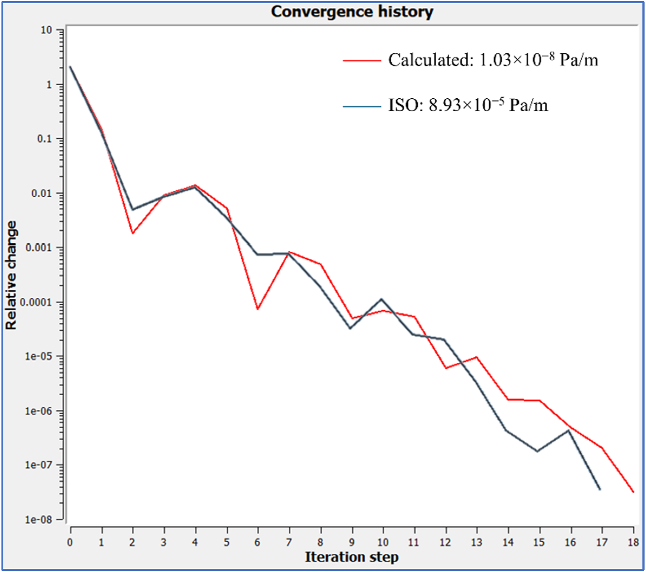

CNOSSOS-EU method and its implementation in Noise Modelling

CNOSSOS-EU method

CNOSSOS-EU was developed during the period 2009–2012 by the European Commission in a cooperative process involving the European Environment Agency, the World Health Organization Europe, the European Aviation Safety Agency and experts appointed by EU countries.^7,14

Its purpose is to provide a common framework to ensure consistency in environmental noise assessment, thus facilitating the implementation of the European Environmental Noise Directive (END). It was approved by the European Commission as Directive (EU) 2015/996 of 19 May 2015 (OJEU No. 168 of 1 July 2015).

Although, according to Directive 2015/996, CNOSSOS-EU comes into force from 2018, the method has been updated, among other things following the document “Amendments for CNOSSOS-EU: Description of issues and proposed solutions⁵²” in which various problems in the mathematical apparatus of CNOSSOS-EU were detected and solutions were proposed.

This revision process resulted in the Commission Delegated Directive (EU) 2021/1226 of 21 December 2020 (OJEU No. 269, of 28 July 2021), which amends the previous one, and regulates the current configuration of the method. CNOSSOS-EU is actually a compendium of calculation methods that can be summarized as:

- Emission calculation methods for:

○ Road traffic.

○ Rail traffic.

○ Industrial noise.

- Method of calculating propagation paths (Ray Tracing):

○ Diffractions.

○ Reflections.

- Propagation calculation method:

○ Divergence attenuation.

○ Attenuation by absorptions.

○ Ground effect attenuation.

○ Diffraction attenuation.

- Calculation methods in receivers.

- Aeronautical noise, that is based on Document no. 29 ECAC.⁵³

In this sense, although CNOSSOS-EU is framed in semi-empirical methods, which involve a simplification of reality to explain a physical phenomenon, it is not a simple model, since each of the previous methods is made up of a large number of algorithms, parameters and conditioning factors, being really complex to implement in software.⁵⁴

Implementation of CNOSSOS in Noise Modelling

Noise Modelling implements CNOSSOS-EU through a series of libraries programmed in JAVA, grouped into⁵⁵:

- “noisemodelling-jdbc” library. Connections to databases that house the geospatial information that determines the acoustic scenario

- “noisemodelling-emission” library: determines the emission power.

- “noisemodelling-pathfinder” library: controls the ray tracing algorithm, reflections, diffractions and propagation conditions.

- “Noisemodelling-propagation” library: determines the set of attenuations (divergence, diffraction, soil, atmosphere, absorptions of structures).

Noise Modelling complies with the ISO 17534-4:2020 standard.⁵ Likewise, it has been verified that the results of Noise Modelling are comparable to those of other widely accepted software in the field of environmental acoustics.^31,56

Simulation scenario

For this work, a standard simulation scenario has been constructed, which has been applied to all calculation methods.

The scenario (Figure 2) includes an omnidirectional noise source, an acoustic screen, and a thick element (building).

Figure 2.

Calculation scenario. Dimensions in meters.

The dimensions of the scenario are:

- Domain width: 42.5 m

- Domain height: 15 m

- Source centroid height: 2 m

- Source diameter: 1 m

- Source power: Lw = 100 decibels (dB), equivalent to 2 Pascals (Pa).

- Supply-screen distance: 4 m

- Screen height: 5 m

- Screen width: 0.3 m

- Screen distance - building: 15 m

- Building dimensions: 10 m high x 8 m wide

The objective of this scenario is to study the propagation of sound with the methodologies indicated above, at different frequencies, and with obstacles to propagation.

Simulations

In the same scenario, simulations have been carried out using the Finite Element Method, with the Wave and Helmholtz equations, and using the CNOSSOS-EU method. Simulations have also been done in the same scenario without noise screen, to obtain insertion loss (IL).

The simulations have the characteristics indicated below.

Common parameters in FEM simulations

To make the results comparable, the following parameters are common in FEM simulations:

- Dimensions of the calculation domain.

- Boundary Conditions:

○ Free exit at the upper limit and sides of the domain.

○ Fully reflective surfaces on the ground, screen and building.

- Propagation speed (c): 343 m/s, that depends on the following parameters:

○ Air density: 1205 kg/m³

○ Temperature: 293 K (20°C)

- Effects of wind are not considered (calm).

In addition, transmission loss (TL) has not been considered, since neither the CNOSSOS-EU method, nor the ISO 9613-2 standard on which it is based, contemplate it.

Parameters in CNOSSOS-EU simulation

To ensure that the simulation parameters are comparable to the FEM simulations, the calculation in CNOSSOS-EU has been configured as follows:

- Compute domain dimensions identical to FEM.

- Fully reflective surfaces on the ground (G = 0), screen and building (α_r = 0).

- Temperature: 293 K (20°C).

- Relative humidity: 0%.

- No. of reflections: 3.

- Diffraction on vertical axis: No.

- Diffraction on horizontal axes: Yes.

The justification for these parameters is derived from the conditions imposed on the FEM model.

Although by default CNOSSOS-EU recommends 70% relative humidity, and 15°C temperature, the air density previously imposed in the FEM simulations is 1205 kg/m3, equivalent to dry air at 20°C, and corresponds to a sound propagation speed of 343 m/s.

Regarding the number of reflections, the effect of increasing their number in this domain has been studied, finding that there are no significant differences in the result with a value greater than 3 reflections.

Diffractions on vertical axes are omitted, since in the FEM model the mesh is 2D, simulating an infinite barrier.

Study frequencies

According to END (last modification in 2021), by default, CNOSSOS-EU considers the center frequencies in octaves, taking 1 kHz as a reference (63 Hz, 125 Hz, 250 Hz, 500 Hz, 1 kHz, 2 kHz, 4 kHz, 8 kHz).

For reasons of simplification of the analysis, and computational cost, the frequencies 125 Hz, 500 Hz and 1 kHz have been selected to carry out the analysis in this work.

Mesh sizes

Typically, the mesh sizes applied in CNOSSOS-Eu and FEM are radically different. In the case of CNOSSOS-EU, the definition of the acoustic scenario (terrain, buildings, propagation conditions, etc.) is of great importance when it comes to obtaining valid results. The mesh size of receivers in which the sound is calculated, particularly in Noise Modelling software, taking the same scenario as a reference, is of minor importance. In other words, a denser mesh of receivers will allow a better representation of the isophones, but the density of the mesh does not interfere with the results of each receiver.⁵⁶

In the case of FEM, spatial discretization in the Wave and Helmholtz equations, and time step size, are decisive to solve the problem. If they are not adequate, they will lead to invalid results, convergence problems, and even impossibility of calculation.^13,22,48,57

To avoid these problems, the observation of the Courant-Friedrichs-Lewy criterion (CFL) is recommended. This criterion provides a necessary condition for the stability and accuracy of the numerical solution, relating the size of the time step ( $Δ$ t) to the size of the spatial mesh ( $Δ$ x), at a given frequency.^13,58

The CFL criterion can be expressed as (equation (12)):

Δ t \leq \frac{Δ x}{c \sqrt{\dim}}

(12)

where:

• dim, is the spatial dimension of the problem (e.g., 1 for one-dimensional, 2 for two-dimensional, etc.).

In this case, the following criteria have been applied in each of the FEM simulations (equation (13)):

Δ t \leq \frac{T}{10} / Δ x \leq \frac{λ}{10}

(13)

These criteria have been applied to the wave with the highest frequency simulated in FEM, this being 1 kHz, resulting in the following spatial and temporal resolution:

• $Δ$ t = 0.0001 s.

• $Δ$ x = 0.0343 m.

These criteria result in obtaining valid simulations in all frequencies studied in FEM.

In the case of CNOSSOS-EU, the model $Δ$ x = 0.06 m has been applied to all calculations.

Results and discussion

Results of the wave equation simulations

The wave equation offers a time series in which the evolution of the wave is observed at each frequency and time step. These results are useful for observing how the wavefront behaves over time within the computational domain, and for the visual study of diffractions and reflections at each frequency.

Figure 3 shows the evolution of the wavefront, at two different moments of the simulation, and for the three frequencies studied. At the frequency of 125 Hz, whose wavelength is 2.74 m, a high diffraction is observed, and the wave overcomes the obstacle with hardly any attenuation. The poor effectiveness of ordinary acoustic screens at low frequencies is a well-known problem that has also been addressed in other works.⁵⁹ However, the 500 Hz and 1 kHz waves have a much less pronounced diffraction, with wavelengths of 0.686 and 0.343 m respectively.

Figure 3.

Comparison of the results of the wave equation, expressed in dB, at the frequencies of 125, 500 and 1000 Hz, at two different times of the FEM simulation.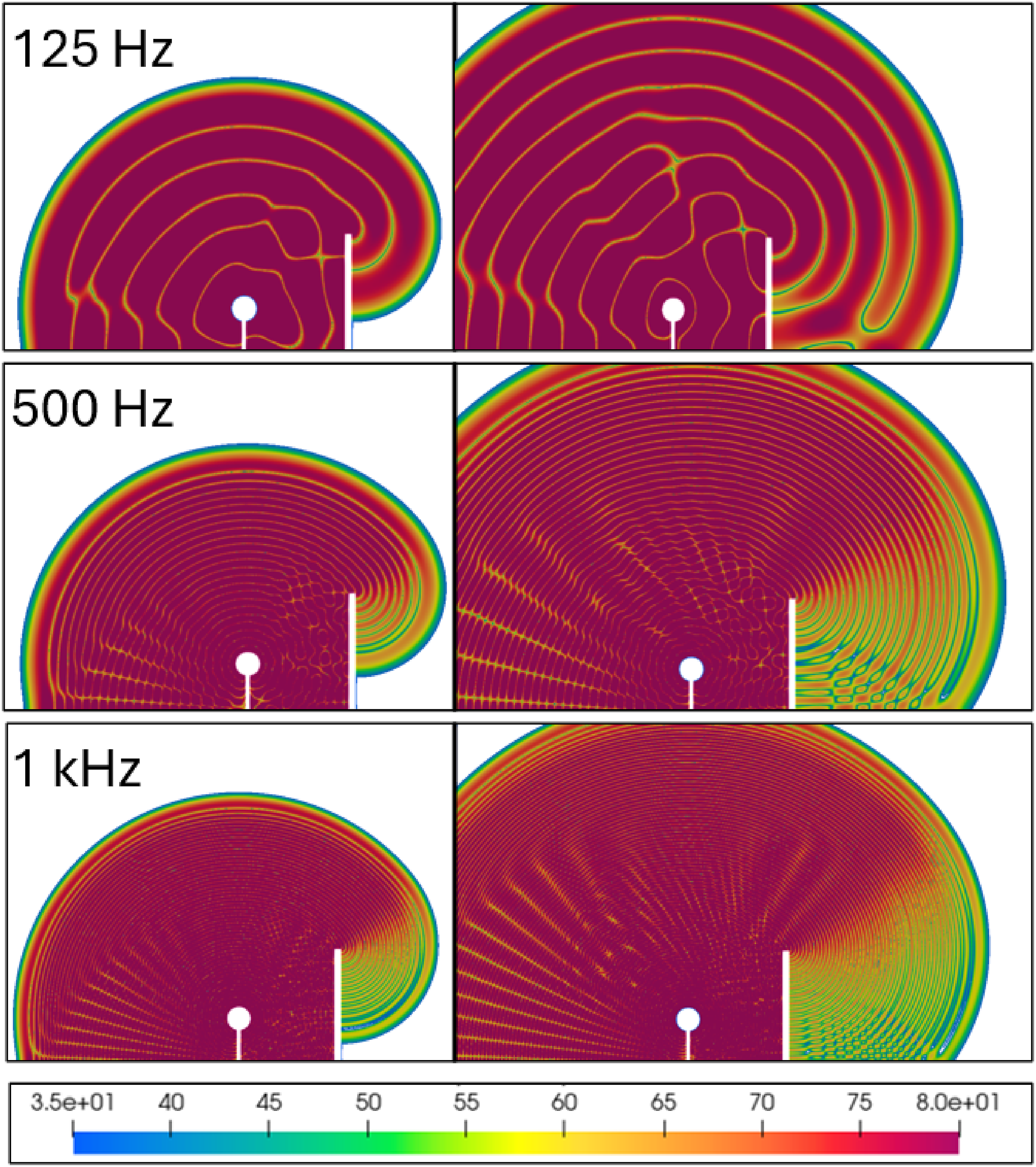

This explains why the attenuation at low frequencies of certain acoustic screens may be insufficient, requiring a more detailed study of their absorbent characteristics or geometry, to give a satisfactory response to the problem they intend to solve. This phenomenon has also been studied in other works.⁶⁰

Although the results of the Wave Equation may be interesting for the study of propagation, they are not really useful for the study of the steady state.⁶¹

For the purposes of this work, its use as a complementary element to CNOSSOS-EU is limited to preliminary phases of the study, in which it is necessary to understand the interaction of the waves with the acoustic environment as a function of time. It could be interesting to simulate different shapes of noise barriers and study the incident wave on them.

Results of the Helmholtz equation simulations

The Helmholtz Equation, on the other hand, does provide the steady state of the acoustic pressure field (P), in the frequency domain. Its result can be interpreted independently of time, as an equilibrium situation representative of the conditions established in the model.

So, it can be valid to establish, in the long term, the acoustic situation of the environment, if the source is characterized in such a way that it is representative of its normal operation over time.

The results allow for the comparison of sound pressure between the different study frequencies.

The Helmholtz equation pressure field

The result of the Helmholtz Equation in Elmer FEM is the pressure field P (Pa), which represents the spatial distribution of sound pressure and describes how it varies throughout the simulated domain (Figure 4).

Figure 4.

Sound pressure field (Pa) at the frequency of 125 Hz, obtained with the Helmholtz equation.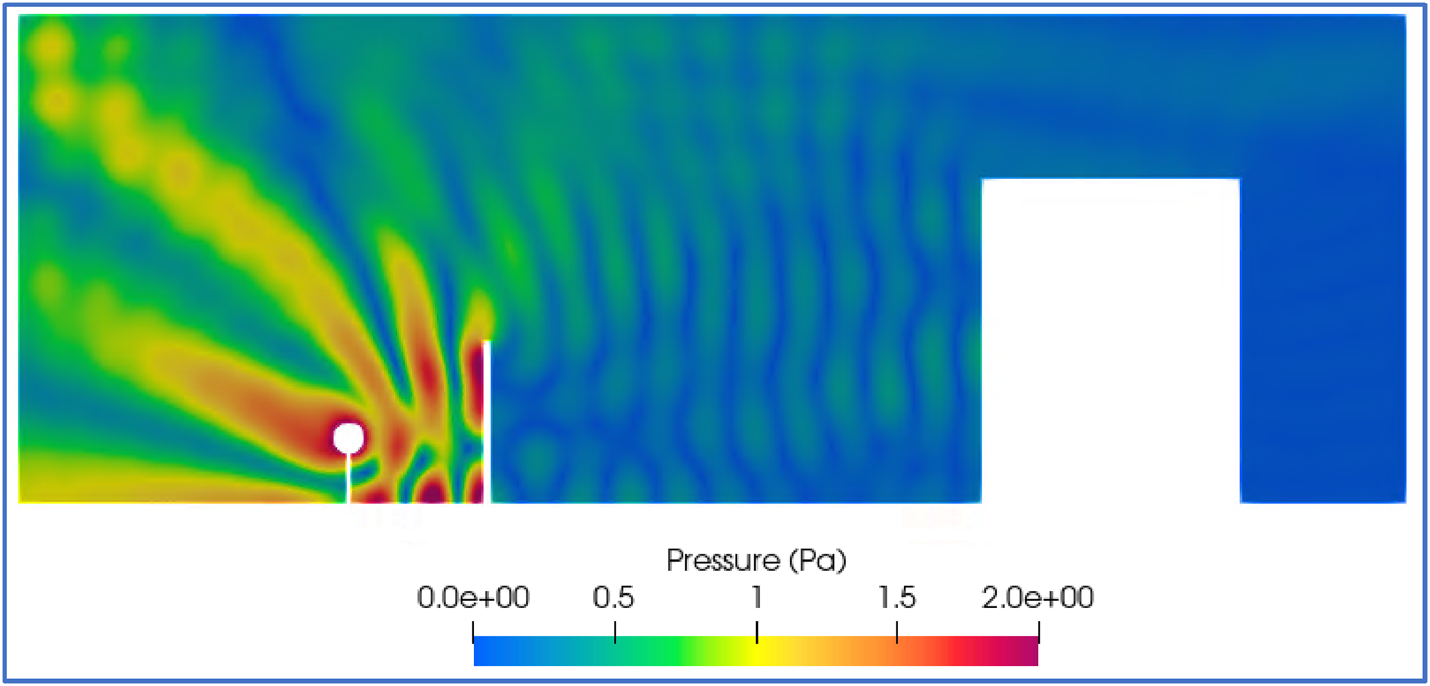

The results are obtained in the form of the real and imaginary parts of the pressure field, which are used to compute the scalar pressure magnitude.

To obtain the magnitude of P field, the next expression (equation (14)) is applied:

P_{m a g n i t u d e} = \sqrt{{P_{r e a l}}^{2} + {P_{i m a g}}^{2}}

(14)

The field P expresses the distribution of the sound pressure caused by the source and its amplitude in Pascals (Pa).

The Helmholtz equation sound pressure level (SPL) assessment

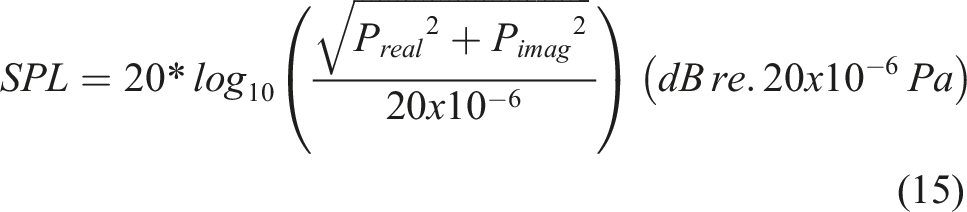
From these results, it is also possible to obtain the SPL value of each frequency in dB, by applying the following expression (equation (15)):

S P L = 20 * \log_{10} (\frac{\sqrt{{P_{r e a l}}^{2} + {P_{i m a g}}^{2}}}{{20 x 10}^{- 6}}) (d B r e . 20 x 10^{- 6} P a)

(15)

The sound pressure levels (SPL) for each of the frequencies show a marked differential behavior between the low (125 Hz) and medium (500 and 1000 Hz) frequencies studied (Figure 5).

Figure 5.

Sound pressure level (dB) at the frequency of 125 Hz and 1 kHz, obtained by transforming the P field to dB. FEM simulation with the Helmholtz equation.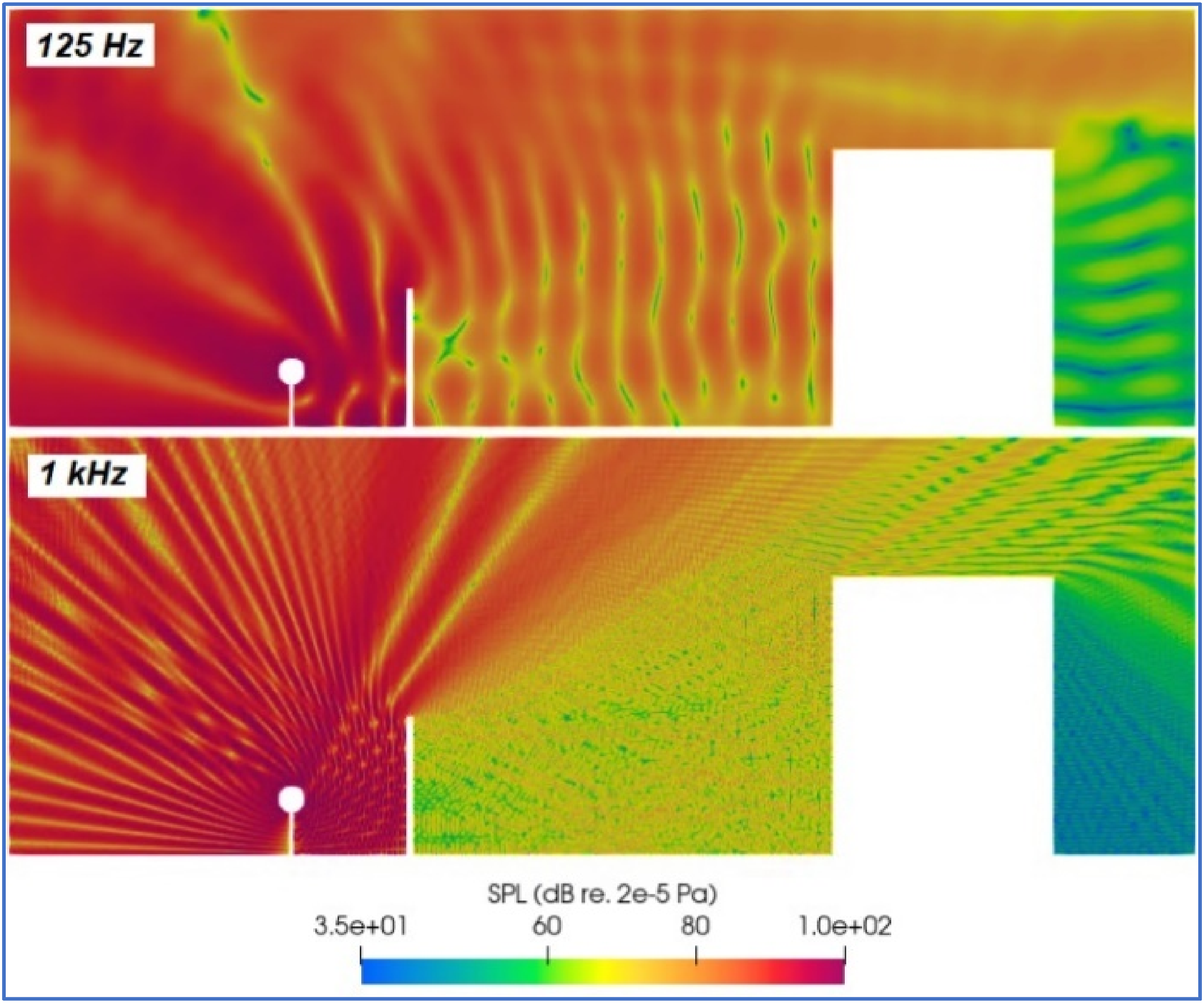

As in the Wave Equation simulations (Figure 3), it is observed that long wavelengths are better at overcoming narrow obstacles than shorter wavelengths.

The SPL values are consistent with the basic formula of the attenuation due to divergence derived from the Helmholtz equation ( $A_{div} = 20 * \log_{10} d$ ), with an increase in the SPL level in the area affected by the screen reflection, and a decrease on the shielded side.

In Figure 6, the behavior of the sound can be observed on both sides of the existing acoustic screen in the model, and in the three frequencies studied.

Figure 6.

Comparison of SPL sound pressure values (in dB) at frequencies of 125, 500 and 1000 Hz, on both sides of the acoustic screen. FEM simulation with the Helmholtz equation.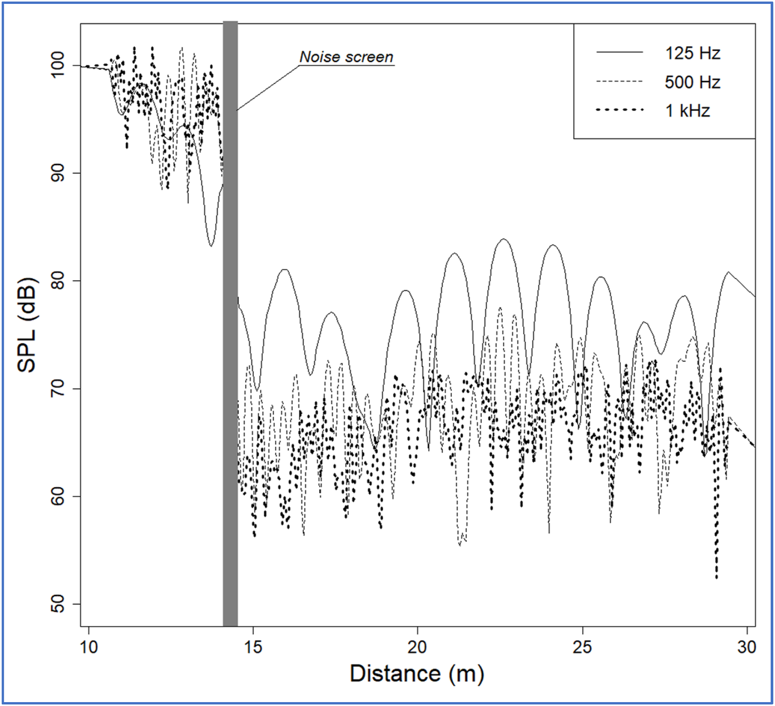

Analogous to what is observed in the results of the Wave Equation, the lower the frequency, the lower the efficiency of the screen. The highest attenuation values are observed at the frequency of 1 kHz (around 30 dB), while at the frequency of 125 Hz the attenuation is around 10 dB.

The Helmholtz equation insertion loss (IL) assessment

Insertion loss (IL) refers to the reduction of the sound pressure level at the point of reception when a barrier is introduced between the noise source and the receiver.⁶²

The evaluation of IL is carried out according to the following general formula:

I L = {L p}_{f r e e} - {L p}_{s c r e e n}

(16)

where:

• Lp_free, is the sound pressure level in the receiver without the barrier.

• Lp_screen is the sound pressure level in the receiver with the barrier.

The results (Figure 7) show attenuations at the frequencies of 125 Hz and 1 kHz, being more pronounced at the highest frequency. The shadow area of the screen, at each frequency, is also different, with the shielding efficiency being lower at the frequency of 125 Hz, specifically in the highest area of the building.

Figure 7.

IL of frequencies 125 and 1 kHz. FEM simulation with the Helmholtz equation.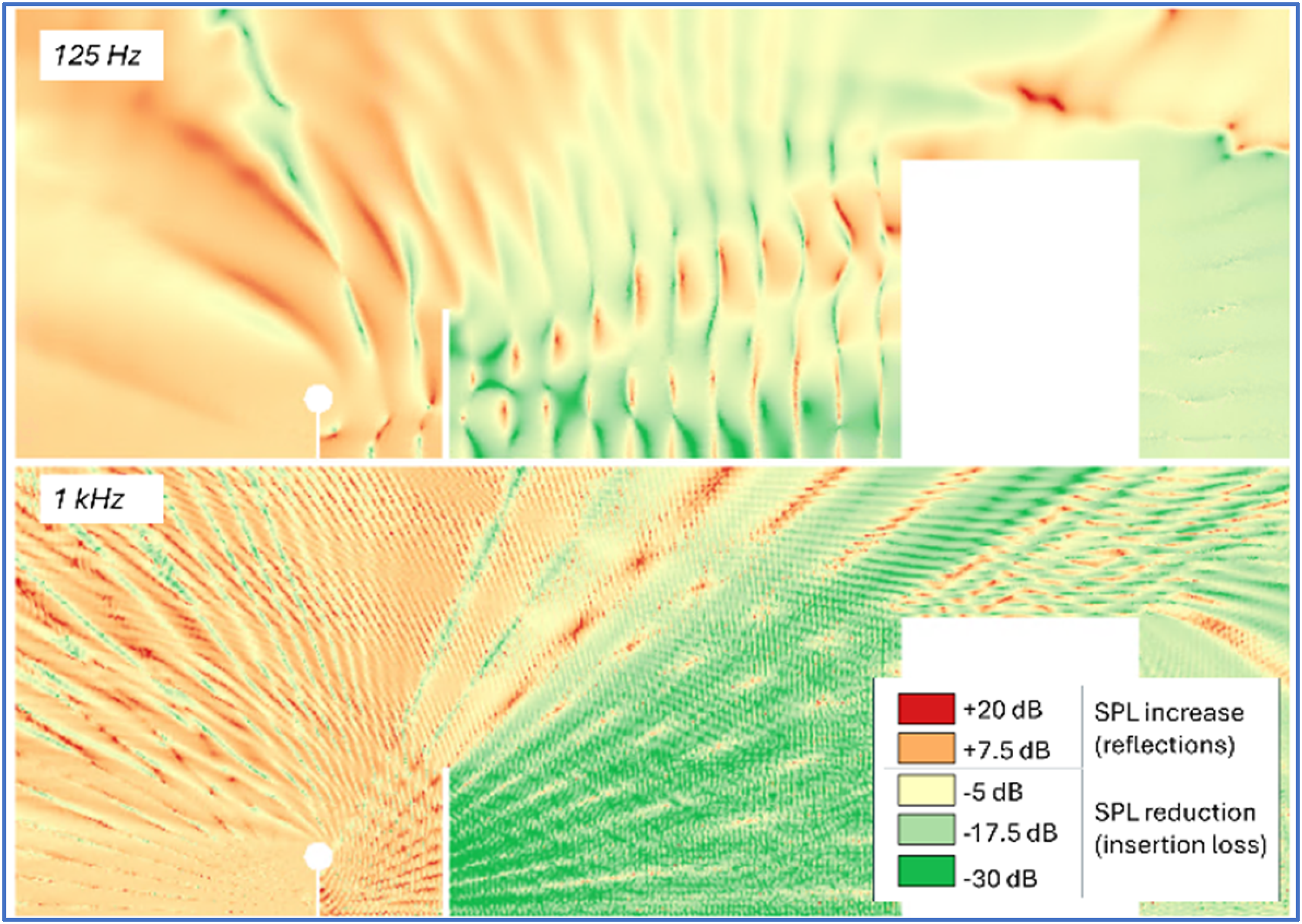

Frequency histograms (Figure 8) of IL attenuation, at each frequency, show a greater range of attenuations as the frequency increases, with the display attenuation range being 0–15 dB for the 125 Hz frequency, and 0–30 dB for the 500 Hz and 1 kHz frequencies.

Figure 8.

Frequency histograms of IL attenuation at the frequencies of 125, 500 and 1000 Hz, calculated from the results of the Helmholtz equation.

Results of CNOSSOS-EU simulations

The simulation results of CNOSSOS-EU, with Noise Modelling software, in accordance with the Environmental Noise Directive, should be long-term, A-weighted average sound levels. Noise Modelling delivers results in each octave, from 63 Hz to 8 kHz in dB, and the equivalent continuous level weighted in dB(A), as the decibel sum of the values of each octave, by evaluation periods (day, evening and night).

It also offers the Lden index, obtained by applying the following equation:

L_{d e n} = 10 \log_{10} \frac{1}{24} (12 * 10^{\frac{L d}{10}} + 4 * 10^{\frac{L e + 5}{10}} + 8 * 10^{\frac{Ln + 10}{10}})

(17)

To calculate the Lden indicator, the afternoon (Le indicator) and night (Ln indicator) periods are penalized with 5 and 10 dB(A), in order to reflect the greater annoyance and the potentially more harmful impact of noise during those periods as opposed to noise during the day (Ld indicator).

For this work, the Ld indicator evaluated by Noise Modelling has been selected, since it implies no penalty and reflects the medium, long-term noise caused by the operation of the source.

An advantage of Noise Modelling compared to other software on the market is that, by default, it offers results by frequencies, in dB, and the equivalent continuous level in dB(A). Therefore, in order to process the results by frequency, no correction is necessary.

The aim is for the results to be analogous to those of the Helmholtz Equation, thus being able to compare both modeling methods.

CNOSSOS-EU pressure field

CNOSSOS-EU is not a method for evaluating sound pressure fields directly. However, it is possible to estimate the Root-Mean-Square (RMS) pressure from the sound pressure levels (SPL) obtained in dB (re.20 × 10⁻⁶ Pa). To compute the RMS pressure in pascals (Pa), the following expression is applied (equation (18)):

P_{R M S} = {20 x 10}^{- 6} * 10^{\frac{L p}{20}} (P a)

(18)

This way of presenting the results of CNOSSOS-EU is not particularly interesting in environmental acoustics, where sound data is typically expressed in dB. However, it could be useful to evaluate how CNOSSOS-EU indirectly calculates the pressure wave field. The comparison of Figures 9 and 4 reveals significant differences. In Figure 4 (FEM simulation), the pressure field shows a complex distribution, whereas in Figure 9 (CNOSSOS-EU) it shows an unrealistic, well-defined decreasing pattern. Additionally, the magnitude of the pressure wave field is around twice higher in FEM simulations.

Figure 9.

Root-mean-square (RMS) pressure (Pa) at the frequency of 125 Hz, obtained by transformation of the CNOSSOS-EU results. Simulation with Noise Modelling software.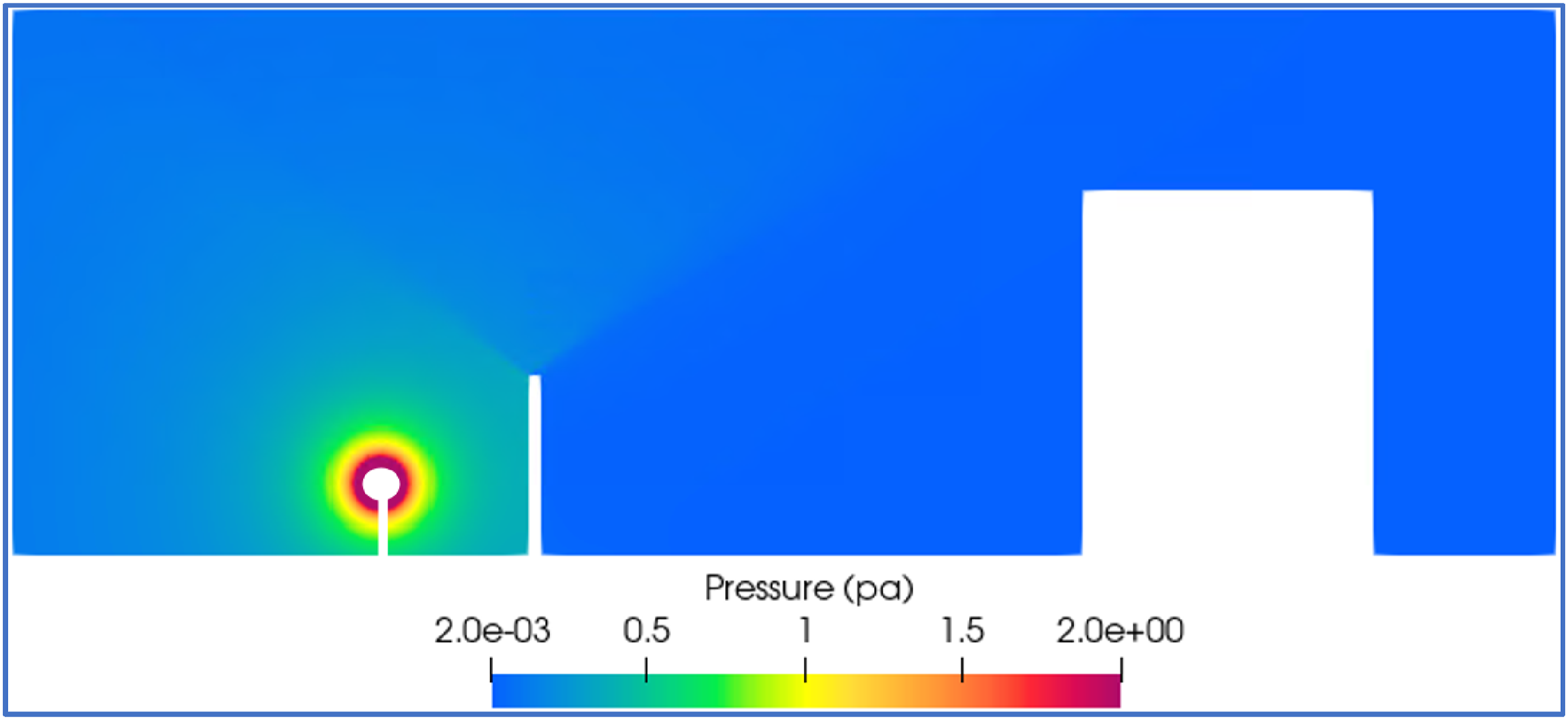

CNOSSOS- EU sound pressure level (SPL) assessment

Similar to the simulations with the Wave and Helmholtz equations, the sound pressure levels (SPL) for each studied frequency show differences between low (125 Hz) and medium (500 and 1000 Hz) frequencies (Figure 10). This demonstrates that shorter wavelengths can better overcome narrow obstacles compared to longer wavelengths.

Figure 10.

SPL results (dB) of the simulation with CNOSSOS-EU with frequencies of 125 and 1 kHz. Effect of the insertion loss of an acoustic screen. Simulation with Noise Modelling software.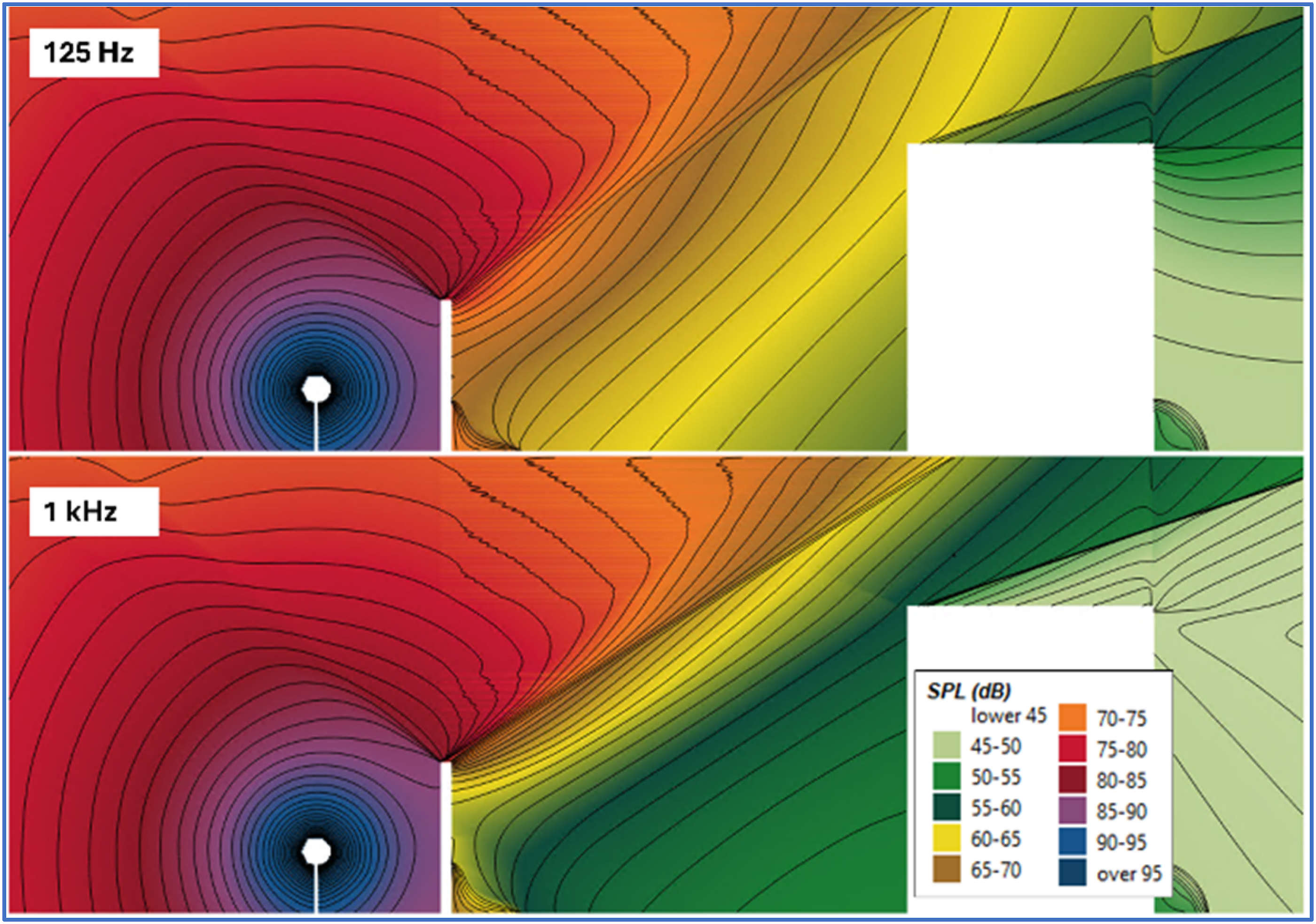

In this case, the SPL values are consistent with the basic formula of divergence attenuation derived from the CNOSSOS-EU method ( $A_{div} = 20 * \log_{10} d + 11$ ), with an increase in SPL level in the area affected by the screen reflection, and a decrease on the shielded side.

In Figure 11, the behavior of the sound can be observed on both sides of the existing acoustic screen in the model, and in the three frequencies studied.

Figure 11.

Comparison of SPL sound pressure values (in dB) at frequencies of 125, 500 and 1 kHz, on both sides of the acoustic screen. CNOSSOS-EU method. Simulation with Noise Modelling software.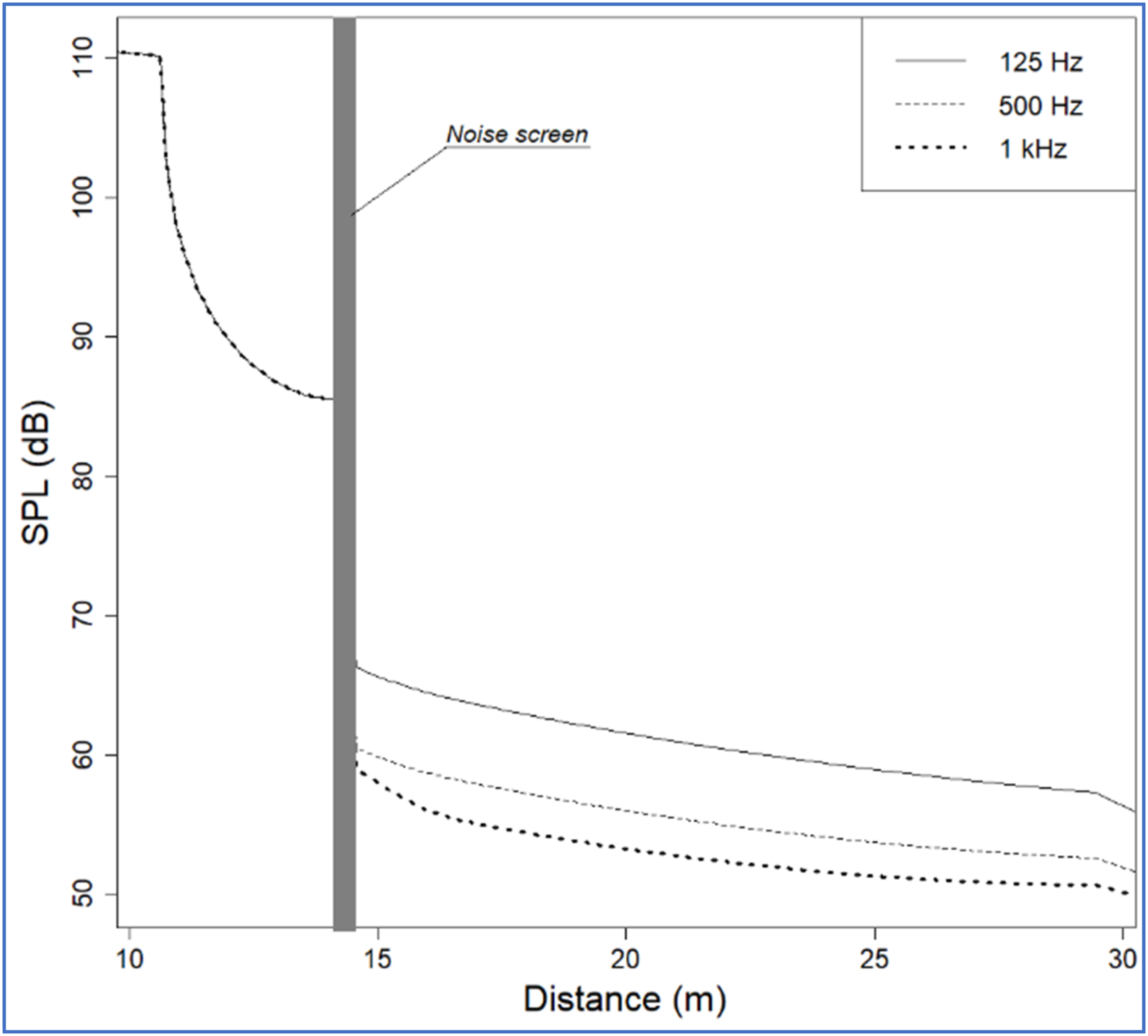

Analogous to what is observed in the results of the Wave Equation and Helmholtz Equation, it is also observed that the screen is less efficient the lower the frequency. Highest attenuation values are observed at the frequency of 1 kHz (around 30 dB), while at the frequency of 125 Hz the attenuation is around 20 dB. But, in the case of Helmholtz Equation, at the frequency of 125 Hz the attenuation is around 10 dB.

CNOSSOS-EU insertion loss (IL) assessment

As in the case of FEM simulations, IL evaluation is performed according to the IL general formula (equation (16)).

The results (Figure 12) show attenuations at the frequencies of 125 Hz and 1 kHz, being more pronounced at the highest frequency. The shadow areas of the screen, at each frequency, are also different in terms of the level of attenuation, and it is observed that, also in CNOSSOS-EU, the shielding efficiency is lower, specifically in the highest area of the building, at the frequency of 125 Hz.

Figure 12.

IL of the frequencies 125 and 1 kHz. CNOSSOS-EU Method. Simulation with Noise Modelling software.

Frequency histograms (Figure 13) of IL attenuation, at each frequency, show a wider range of attenuations as the frequency increases, with the display attenuation range being 0-15 dB for the 125 Hz frequency, 0-20 dB for the 500 Hz frequency, and 0 to 25 dB for the 1 kHz frequency.

Figure 13.

Frequency histograms of IL attenuation at the frequencies of 125, 500 and 1000 Hz, using the CNOSSOS-EU method. Simulation with Noise Modelling software.

Comparison of CNOSSOS-EU and FEM results

A comparative analysis of results between the Helmholtz Equation and the CNOSSOS-EU method has been carried out, in order to determine the differences in the results of both, as well as their explanation.

We have compared the results in SPL and IL, for each frequency studied.

Comparison of SPL sound levels on scenario with barrier

First, the comparison of histograms is carried out (Figure 14). Graphically, significant differences are observed between the histograms, due to a higher frequency of lower values in the CNOSSOS-EU histograms compared to the Helmholtz histograms. That means that attenuation in CNOSSOS-EU is much higher than in FEM Helmholtz Equation simulation.

Figure 14.

Comparison of SPL frequency histograms at 125, 500 and 1000 Hz, with the CNOSSOS-EU method and with Helmholtz. Scenario with acoustic barrier.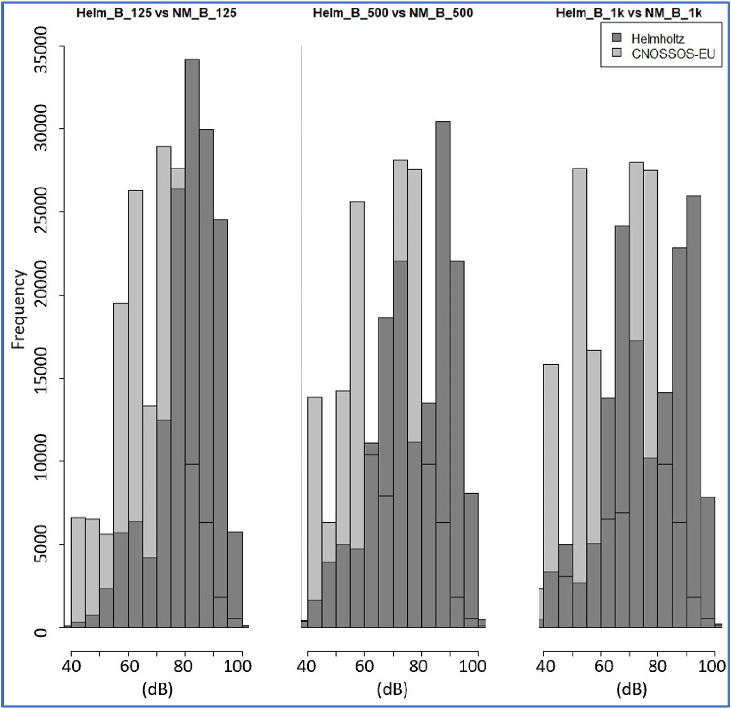

In addition, the statistical tests of Kolmogorov-Smirnov (KS Test), Mann-Whitney (MW Test) and Pearson’s Correlation Coefficient have been applied, in order to study whether the distributions and medians of the samples are different, as well as the correlation between them. The results are shown in Table 1.

Table 1.

Statistical tests of Kolmogorov-Smirnov (KS Test), Mann-Whitney (MW Test) and Pearson’s correlation coefficient, to the results of SPL of the Helmholtz equation and CNOSSOS-EU, in a scenario with acoustic barrier.

Freq	KS stat	MW stat	Correlation
125 Hz	0.53	19 × 10⁹	0.865
500 Hz	0.37	16 × 10⁹	0.917
1 kHz	0.35	16 × 10⁹	0.919

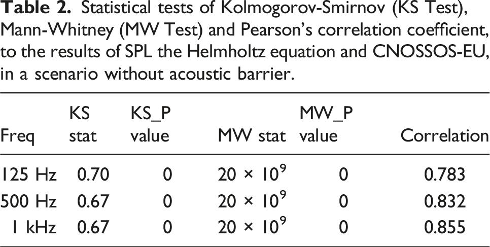
These tests indicate that the Helmholtz Equation and CONOSSOS-EU datasets are statistically different (Kolmogorov-Smirnov (KS Test), Mann-Whitney (MW Test)) in their distributions and medians, but are highly correlated (Pearson’s Correlation Coefficient), meaning they have a strong linear relationship, and suggesting that the data tend to vary in the same direction.

Comparison of SPL sound levels in a barrier-free scenario

Comparing the results in the scenario without an acoustic barrier, the same trend is followed (Figure 15). The results of CNOSSOS-EU (NM) show a more pronounced distribution toward lower SPL ranges.

Figure 15.

Comparison of SPL frequency histograms at 125, 500 and 1000 Hz, with the CNOSSOS-EU method and with Helmholtz. Scenario without acoustic barrier.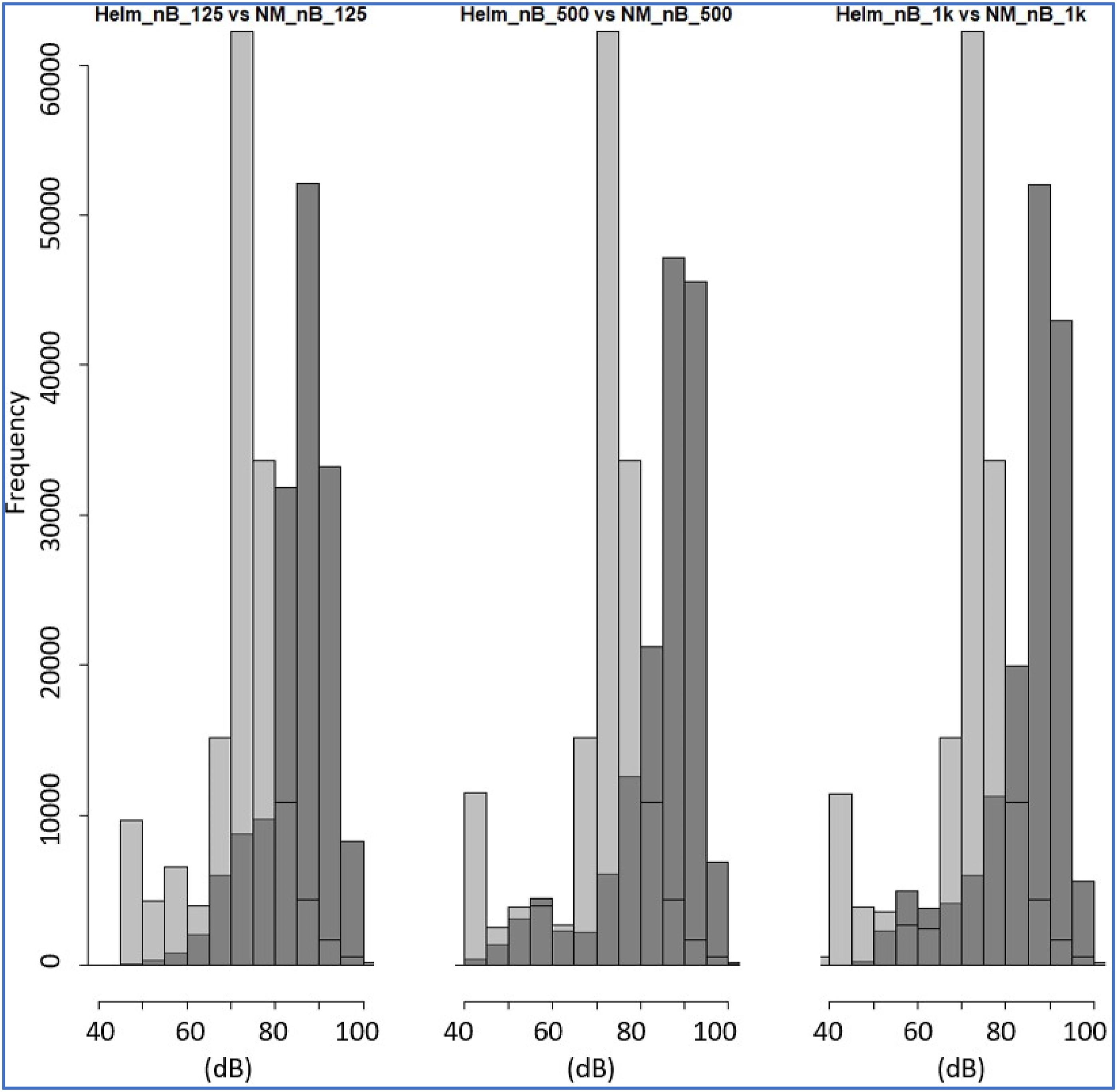

Applied statistical tests indicate that the Helmholtz Equation and CONOSSOS-EU datasets are also statistically different (Table 2), in this scenario, in their distributions and medians, although they are also highly correlated.

Table 2.

Statistical tests of Kolmogorov-Smirnov (KS Test), Mann-Whitney (MW Test) and Pearson’s correlation coefficient, to the results of SPL the Helmholtz equation and CNOSSOS-EU, in a scenario without acoustic barrier.

Freq	KS stat	MW stat	Correlation
125 Hz	0.70	20 × 10⁹	0.783
500 Hz	0.67	20 × 10⁹	0.832
1 kHz	0.67	20 × 10⁹	0.855

Comparison of insertion losses

Comparing the histograms of insertion losses (IL), it can be observed that, although the values distribution is different, they present a same increasing tendency as the frequency studied also increases (Figure 16).

Figure 16.

Comparison of frequency histograms of IL attenuation at 125, 500 and 1000 Hz, with the CNOSSOS-EU method and with Helmholtz. Scenario with acoustic barrier.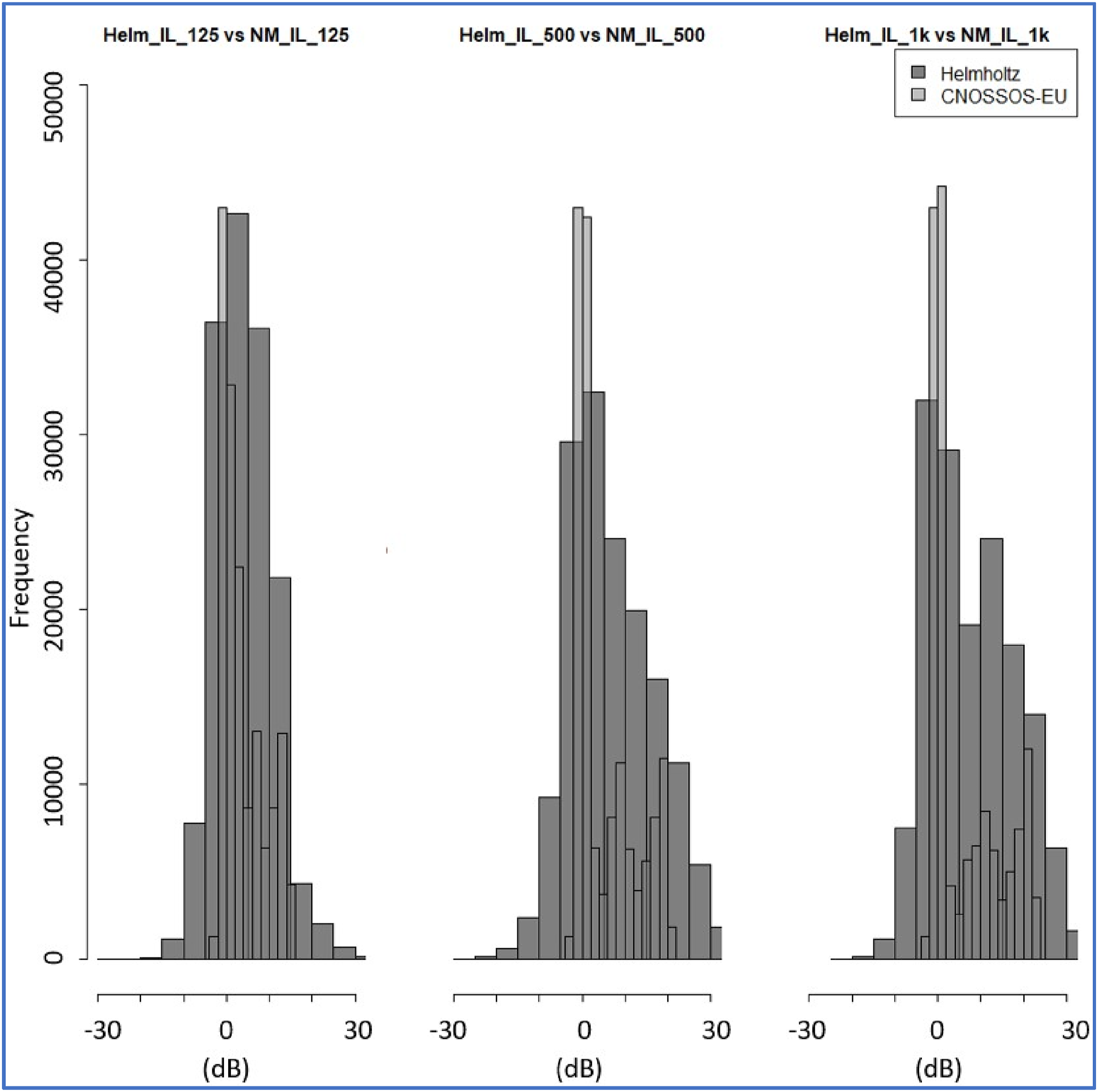

Statistical tests (Table 3) indicate that, although the Helmholtz and CNOSSOS distributions and medians for the IL (Insertion loss) dataset are significantly different, the data for 500 Hz and 1 kHz show a strong correlation, while the data for 125 Hz show a moderate correlation. This suggests that, although there are differences in distribution, the Helmholtz and CNOSSOS-EU values tend to vary together for the 500 Hz and 1 kHz frequencies, but less so for 125 Hz.

Table 3.

Statistical tests of Kolmogorov-Smirnov (KS Test), Mann-Whitney (MW Test) and Pearson’s correlation coefficient, to the results of IL of the Helmholtz equation and CNOSSOS-EU, in a scenario without acoustic barrier.

Freq	KS_statistic	MW_statistic	MW_p_value	Correlation
125 Hz	0.15	12 × 10⁹	8.0 × 10⁻¹²⁵	0.589
500 Hz	0.21	13 × 10⁹	0	0.788
1 kHz	0.22	13 × 10⁹	0	0.793

Interpretation of differences between FEM and CNOSSOS-EU simulations

There are two fundamental differences between the results of the Helmholtz Equation and the CNOSSOS-EU method.

The first one has to do with the sound pressure level (SPL) in the calculation domain. In the case of Helmholtz, the resulting SPL, on average, is higher than that of the CNOSSOS-EU method.

This difference is mainly by reason of the treatment of attenuation due to sound divergence. In the CNOSSOS-EU method, the geometric divergence attenuation, Adiv, corresponds to a reduction in the equivalent continuous sound pressure level due to the propagation distance. If it is a point sound source in the free field, the attenuation in dB is obtained from Adiv CNOSSOS-EU Equation (equation (19)):

A_{div} = 20 \times \log_{10} (d) + 11

(19)

The divergence attenuation derived from the Helmholtz Equation can also be calculated by considering a point source of sound that emits spherical waves. In this case, the sound pressure P at a distance d from the source is described by P(d) = A/d, where A is a constant. Converting this sound pressure to sound pressure level in decibels (dB), yields Lp(d) = 20 log10(P(d)/pref), which can be simplified to Lp(d) = Lp(1) - 20 log10(d), where Lp(1) is the sound pressure level at 1 m from the source.

The resulting divergence attenuation equation (Adiv) is defined as (equation (20)):

A_{div} = 20 \times \log_{10} (d)

(20)

Therefore, CNOSSOS-EU increases the attenuation by geometric divergence by means of a parameter K = 11 dB. This practice is common in empirical methods, where the Adiv equation is usually written as follows:

A_{div} = 20 \times \log_{10} (d) + K

(21)

K is a constant used to adjust this formula to different methods and environments, which can consider additional factors specific to each method, such as additional absorption, ground reflection, etc.

In fact, this constant adopts a different value depending on the method that is applied. Here are some examples of road noise calculation methods, and the value assumed for the constant K:

• Nordic Prediction Method (Kilde Report 130), applies K = 10⁶³;

• FHWA Traffic Noise Model (TNM), applies K = 11.3⁶⁴;

• NMPB-Routes-96 (French Road Traffic Noise Prediction Method), applies K = 8⁶⁵;

• Austrian Standard ÖAL 28 (Austrian Road Traffic Noise Prediction Method), applies K = 9⁶⁶;

The consideration of the constant (K) in empirical methods is a great difference with respect to the Helmholtz Equation, causing a more pronounced attenuation, which Helmholtz does not contemplate.

The second difference has to do with the representation of the field of sound levels in the domain, with the result that the calculation of the SPL level at each discrete point of the domain is also different between both methods. The CNOSSOS-EU method, and semi-empirical methods in general, tend to a homogeneous propagation of sound, avoiding sudden level jumps between points that are nearby.

On the contrary, the result of the Helmholtz Equation is a field of pressures that captures the complexities of the acoustic phenomenon, therefore, its representation is not homogeneous.

In addition, the differences obtained have different magnitudes depending on the frequency studied. A greater discrepancy is observed in low frequencies (e.g. 125 Hz) than in high frequencies.

The reason why CNOSSOS-EU presents greater differences with respect to models that better represent the physical reality of the acoustic phenomenon, such as Helmholtz, may lie in the purpose of its design.

CNOSSOS-EU is not designed for a detailed frequency analysis, but to obtain a long-term equivalent continuous level (LAeq), in the different evaluation periods. In other words, the calculation speed and the accuracy of the total noise result (dBA) are prioritized over the accuracy of the frequency analysis.

Although some of the CNOSSOS-EU algorithms depend on the frequency of study, as is the case with atmospheric attenuation, those that have greater weight in the result, such as Adiv, behave in the same way at all frequencies, and are not able to adequately model the physical phenomenon of sound propagation for each one.

If the A-weighting is also taken into consideration, it is observed that low frequencies, such as 125 Hz, have a much more pronounced penalty (−16.1 dB) than medium frequencies, such as 500 Hz (−3.2 dB), and 1 kHz (0.0 dB). Its contribution to the LAeq is therefore much less important, and the errors in its calculation, considering the purpose of CNOSSOS-EU, are negligible.

Conclusions

This study concludes that applying the Finite Element Method (FEM), specifically through the Helmholtz and Wave Equations, offers valuable insights into addressing limitations of the CNOSSOS-EU method in complex acoustic environments.

FEM-based approaches (Helmholtz and Wave equations)

The FEM approach allows for precise modeling of sound propagation and attenuation, particularly beneficial in scenarios where high spatial resolution is essential, such as the design of acoustic barriers. Within FEM, the Helmholtz and Wave Equations each serve distinct purposes:

• The Wave Equation provides a time-domain solution that captures the dynamic evolution of the wavefront, allowing the observation of acoustic phenomena such as diffraction and reflection, which shape the acoustic environment.This temporal approach is particularly useful in scenarios where changes over time, such as atmospheric turbulence and wind profile variations, significantly impact sound behavior.

• The Helmholtz Equation offers a frequency-domain, time-independent result, represented as a pressure field. This result can be transformed into scalar pressure fields in decibels, facilitating detailed frequency-specific analysis in a single acoustic environment. The Helmholtz approach allows for comparison with other standard methods in environmental noise, providing a deeper understanding of differential behavior across frequencies.

CNOSSOS-EU

In contrast, CNOSSOS-EU is a semi-empirical method designed for large-scale, long-term noise assessment. It uses statistical models and simplifications to generate A-weighted equivalent continuous noise levels (LAeq) that represent typical noise source operations over extended periods. CNOSSOS-EU offers several advantages in efficiency and lower computational demand. However, it relies on generalized assumptions, such as uniform atmospheric conditions and specific propagation constraints, which may limit its accuracy in detailed, small-scale acoustic assessments.

Comparison of results

The comparative analysis between the Helmholtz Equation (FEM-based) and CNOSSOS-EU demonstrates noticeable differences in sound pressure levels (SPLs) across calculation domains. However, strong correlations in SPL pattern trends indicate similar directional changes, showing that both methods achieve convergence in magnitude and SPL variation direction, both in simple (no-barrier) and complex (with-barrier) environments.

Main conclusions

• The Helmholtz and Wave Equations, both FEM variants, offer high accuracy in modeling sound propagation physics, with the Helmholtz approach suited for frequency-domain studies and the Wave Equation effective for examining time-variant acoustic interactions.

• The Wave Equation enables detailed visualization of transient wave phenomena (reflection and diffraction), while the Helmholtz Equation provides a detailed frequency-based analysis that complements common environmental noise methods.

• CNOSSOS-EU, based on ray tracing, provides a computationally efficient approximation suitable for strategic noise mapping over large areas. However, it may lack precision in frequency-specific and detailed analyses, particularly at low frequencies.

• Both methods are complementary: CNOSSOS-EU is well-suited for broad noise mapping, whereas FEM-based methods, especially in complex acoustic scenarios, provide the high resolution necessary for nuanced assessments and detailed noise control strategies.

This study highlights the value of combining CNOSSOS-EU with FEM-based methods to enhance the accuracy of noise assessments and develop more effective noise control strategies. Given the limitations of CNOSSOS-EU in detailed studies and complex acoustic environments, we recommend a review of the Environmental Noise Directive. Such a review would allow competent authorities to recognize these limitations and consider supplementary methodologies, ensuring more accurate and comprehensive noise assessments in diverse environmental contexts.

Footnotes

Acknowledgements

We would like to express our gratitude for the contributions and assistance received from the following individuals and entities: Pierre Aumond and Nicolas Fortin, from the Joint Research Unit in Environmental Acoustics (UMRAE - France), for their help in resolving questions and handling the Noise Modelling software. People of the Elmer FEM forum⁶ community for their support in resolving questions and handling the Elmer FEM software. María Díaz Redondo, PhD in Nature-Based Solutions and linguist, for her help in reviewing the English version of the text and ensuring compliance with the journal’s requirements. Celia Moreno Molina, PhD in Telecommunications, for her review of the presentation of the Helmholtz and Wave equations in this work.

Author contributions

Ignacio Soto Molina: Conceptualization; Data curation; Formal analysis; Investigation; Methodology; Project administration; Resources; Software; Writing – original draft. Miguel Ausejo Prieto: Writing – review and editing; Validation. Rosa María Arce Ruiz: Writing – review and editing; Validation.

Declaration of conflicting interests

The author(s) declared no potential conflicts of interest with respect to the research, authorship, and/or publication of this article.

Funding

The author(s) received no financial support for the research, authorship, and/or publication of this article.

ORCID iDs

Ignacio Soto-Molina

Miguel Ausejo Prieto

Rosa Maria Arce Ruiz

Notes

References

Guski

Schreckenberg

Schuemer

. WHO environmental noise guidelines for the European region: a systematic review on environmental noise and annoyance. Int J Environ Res Public Health 2017; 14(12): 1539. DOI: 10.3390/ijerph14121539.

Basner

Babisch

Davis

, et al. Auditory and non-auditory effects of noise on health. Lancet 2014; 383(9925): 1325–1332. DOI: 10.1016/S0140-6736(13)61613-X.

Münzel

Sørensen

Gori

, et al. Environmental stressors and cardio-metabolic disease: part II–mechanistic insights. Eur Heart J 2016; 38: 557–564. DOI: 10.1093/eurheartj/ehw294.

Basner

McGuire

. WHO environmental noise guidelines for the European region: a systematic review on environmental noise and effects on sleep. Int J Environ Res Public Health 2018; 15(3): 519. DOI: 10.3390/ijerph15030519.

Clark

Paunovic

. WHO environmental noise guidelines for the European region: a systematic review on environmental noise and quality of life, wellbeing and mental health. Int J Environ Res Public Health 2018; 15(11): 2400. DOI: 10.3390/ijerph15112400.

van Kempen

Casas

Pershagen

, et al. WHO environmental noise guidelines for the European region: a systematic review on environmental noise and cardiovascular and metabolic effects: a summary. Int J Environ Res Public Health 2018; 15(2): 379. DOI: 10.3390/ijerph15020379.

Kephalopoulos

Paviotti

Anfosso-Lédée

. Common noise assessment methods in Europe (CNOSSOS-EU) [online]. Luxembourg: European Commission, 2012. DOI: 10.2788/32029.

Rasmussen

Arranz

. The insertion loss of screens under the influence of wind. J Acoust Soc Am 1998; 104(5): 2692–2698.

Ghangale

Colaço

Alves Costa

, et al. A methodology based on structural finite element method-boundary element method and acoustic boundary element method models in 2.5D for the prediction of reradiated noise in railway-induced ground-borne vibration problems. J Vib Acoust 2019; 141(3): 031011. DOI: 10.1115/1.4042518.

10.

Papadakis

Stavroulakis

. Finite element method for the estimation of insertion loss of noise barriers: comparison with various formulae (2D). Urban Sci 2020; 4(4): 77. DOI: 10.3390/urbansci4040077.

11.

Prinn

. A review of finite element methods for room acoustics. Acoustics 2023; 5(2): 367–395. DOI: 10.3390/acoustics5020022.

12.

Asadzadeh

. An introduction to the finite element method (FEM) for differential equations, 2016.

13.

Marburg

Nolte

. Computational acoustics of noise propagation in fluids - finite and boundary element methods. Berlin, Heidelberg: Springer, 2008. DOI: 10.1007/978-3-540-77448-8.

14.

Kephalopoulos

Paviotti

Anfosso-Lédée

, et al. Advances in the development of common noise assessment methods in Europe: the CNOSSOS-EU framework for strategic environmental noise mapping. Sci Total Environ 2014; 482–483: 400–410. DOI: 10.1016/j.scitotenv.2014.02.031.

15.

Bertellino

Gerola

Clementel

, et al. Noise Mapping of Agglomerations: a comparison of interim standards vs. new CNOSSOS method in a real case study. In: INTER-NOISE and NOISE-CON congress and conference proceedings. Hamburg, Germany: Institute of Noise Control Engineering, 2016.

16.

Bañuelos-Irusta

Bañuelos-Arteagoitia

Tomás-Garrido

, et al. Measurements on real urban traffic noise demand higher accuracy on local data to get a representative application of Cnossos-EU. In: INTER-NOISE and NOISE-CON congress and conference proceedings. Madrid: Institute of Noise Control Engineering, 2019.

17.

Venkataraman

Rumpler

Leth

, et al. Improving strategic noise mapping of railway noise in Europe: refining CNOSSOS-EU calculations using TWINS. Sci Total Environ [online] 2022; 839: 156216. DOI: 10.1016/j.scitotenv.2022.156216.

18.

Lauderdale

Economou

Brittain

, et al.

Accuracy of wave based calculation methods compared to ISO 9613-2

[online]. In: NOISE-CON 2014, Fort Lauderdale, Florida, 8–10 September 2014. Available at: https://www.researchgate.net/publication/291345801_Accuracy_of_wave_based_calculation_methods_compared_to_ISO_9613-2 (2014, accessed 12 May 2024).

19.

van der Eerden

Kurylek

Blaak

, et al. Additional noise reduction with diffracting elements on barriers using numerical and standard calculation methods. In: INTER-NOISE and NOISE-CON congress and conference proceedings, Washington, DC, USA, 1–5 August 2021, pp. 3118–3129.

20.

Milbradt

Abed

. Generalized stabilization techniques in computational fluid dynamics 2008.

21.

Vorländer

. Auralization: fundamentals of acoustics, modelling, simulation, algorithms and acoustic virtual reality. Berlin, Heidelberg: Springer Berlin Heidelberg, 2008. DOI: 10.1007/978-3-540-48830-9.

22.

Diwan

Mohamed

. Iterative solution of Helmholtz problem with high-order isogeometric analysis and finite element method at mid-range frequencies. Comput Methods Appl Mech Eng 2020; 363: 112855. DOI: 10.1016/j.cma.2020.112855.

23.

Boue

Boden

Karasalo

. Outdoor sound propagation using an exact finite element method. In: 7th AIAA/CEAS aeroacoustics conference and exhibit, Maastricht, Netherlands, 28–30 May 2001, 2001, p. 2261.

24.

Zhou

Y-Q

Luo

W-Y

. A finite element model for underwater sound propagation in 2-D environment. J Mar Sci Eng 2021; 9(9): 956.

25.

Arnaud

. Flaws in the Cnossos calculation method and proposed solutions. In: 23rd International congress on acoustics. Aachen: Universitätsbibliothek der RWTH, 2019.

26.

Rosão

Leonardo

Santos

. Necessary adjustments in ISO 9613-2 and CNOSSOS (industries) methods for noise forecasting in Wind Farms. Portugal: Environoise, Faro, 2021 [online] Available at: https://documentacion.sea-acustica.es/publicaciones/Madeira21/ID214.pdf (accessed 22 August 2023).

27.

Balogh

Schmelz

Orosz

. Sensitivity of CNOSSOS-EU sound propagation model to digital surface components. Acta Tech Jaurinensis 2022; 15(1): 47–57. DOI: 10.14513/actatechjaur.00644.

28.

Faulkner

J-P

Murphy

. Road traffic noise modelling and population exposure estimation using CNOSSOS-EU: insights from Ireland. Appl Acoust 2022; 192: 108692. DOI: 10.1016/j.apacoust.2022.108692.

29.

Hartog Van Banda

. The three methods of calculating population exposure according to CNOSSOS-EU. In: INTER-NOISE and NOISE-CON congress and conference proceedings, 2023, pp. 3999–4005 [online]. DOI: 10.3397/IN_2022_0570.

30.

Phillips

Trow

Shilton

. Sensitivity of input parameter on CNOSSOS-EU railway emission levels. In: INTER-NOISE and NOISE-CON congress and conference proceedings, 2023, pp. 4698–4705 [online]. DOI: 10.3397/IN_2022_0679.

31.

Soto-Molina

Simón Otegui

Ausejo Prieto

, et al. Análisis comparativo de softwares de simulación de ruido ambiental: comparación entre una solución comercial y una de código abierto. In: 54º Congreso Español de Acústica Tecniacústica [online]. Cuenca: Sociedad Española de Acústica, 2023. Available at: https://documentacion.sea-acustica.es/publicaciones/Cuenca23/Abs_46.pdf (accessed 21 April 2024).

32.

Salomons

Eisses

van Der Eerden

. Effects of tilted noise barriers on road traffic noise. In: Forum acusticum, Lyon, France, December 2020, pp. 439–446.

33.

D’Alembert

JLR

. Recherches sur la courbe que forme une corde tendue mise en vibration. Histoire de l’Académie Royale des Sciences et Belles-Lettres de Berlin pour l’année 1747; 1750: 214–219.

34.

Lynch

Gray

. A wave equation model for finite element tidal computations. Comput Fluids 1979; 7(3): 207–228.

35.

Helmholtz

. Wissenschaftliche Abhandlungen. Leipzig: JA Barth, 1882.

36.

Appelo

Garcia

Runborg

. WaveHoltz: iterative solution of the Helmholtz equation via the wave equation. SIAM J Sci Comput 2020; 42(4): A1950–A1983.

37.

Appel

. Some techniques for shading machine renderings of solids. In: Proceedings of the April 30–May 2, 1968, spring joint computer conference, Atlantic City, New Jersey, 1968, pp. 37–45.

38.

Hofmann

. Who invented ray tracing? Vis Comput 1990; 6(3): 120–124. DOI: 10.1007/BF01911003.

39.

Aumond

Fortin

Can

. Overview of the NoiseModelling open-source software version 3 and its applications. In: INTER-NOISE and NOISE-CON congress and conference proceedings, 2020, pp. 2005–2011.

40.

Råback

Malinen

. Elmer documentation: overview of Elmer [online] Available at: https://www.elmerfem.org/blog/documentation/ (2023, accessed 4 April 2024).

41.

Aumond

Cariou

Chiello

, et al.

Strategic noise mapping in France to 2023: coupling a national database with the open-source software NoiseModelling

[online] Available at: https://www.researchgate.net/publication/362733377_Strategic_noise_mapping_in_France_to_2023_Coupling_a_national_database_with_the_open-source_software_NoiseModelling (2022, accessed 29 August 2023).

42.

UMRAE

Lab-STICC.

Noise Modelling software scientific production

[online] Available at: https://noisemodelling.readthedocs.io/en/latest/Scientific_production.html (2022, accessed 24 August 2023).

43.

Demanet

. Topics in applied mathematics: waves and imaging [online]. MIT OpenCourseWare 2015, Available at: https://ocw.mit.edu/courses/mathematics/18-325-topics-in-applied-mathematics-waves-and-imaging-fall-2015/ (accessed 8 June 2024).

44.

Kinsler

Frey

Coppens

, et al. Fundamentals of acoustics. John Wiley & Sons, 2000.

45.

Griffiths

Schroeter

. Introduction to quantum mechanics. Cambridge University Press, 2018.

46.

Raback

Malinen

Ruokolainen

, et al.

Elmer documentation: models manual

[online] Available at: https://www.nic.funet.fi/pub/sci/physics/elmer/doc/ElmerModelsManual.pdf (2023, accessed 7 April 2024).

47.

Pierce

. Acoustics: an introduction to its physical principles and applications. Springer, 2019.

48.

Kechroud

Soulaimani

Saad

, et al. Preconditioning techniques for the solution of the Helmholtz equation by the finite element method. Math Comput Simulat 2004; 65(4–5): 303–321. DOI: 10.1016/j.matcom.2004.01.004.

49.

Pierce

. Acoustics: An Introduction to Its Physical Principles and Applications. Physics Today, 1989.

50.

Peters

MCAM

Hirschberg

Reijnen

, et al. Damping and reflection coefficient measurements for an open pipe at low Mach and low Helmholtz numbers. J Fluid Mech 1993; 256(1): 499–534, [online] Available at: https://pure.tue.nl/ws/portalfiles/portal/4382792/605459.pdf (accessed 12 May 2024).

51.

ISO 9613-1 . Acoustics — Attenuation of sound during propagation outdoors — Part 1: calculation of the absorption of sound by the atmosphere. ISO - International Organization for Standardization. Working group ISO/TC 43/SC 1 - Noise. ISO standards series of the International Standardization Organization, 1993.

52.

Kok

van Beek

. Amendments for CNOSSOS-EU : Description of issues and proposed solutions. Rijksinstituut voor Volksgezondheid en Milieu RIVM 2019 [online] DOI: 10.21945/RIVM-2019-0023.

53.

ECAC.CEAC Doc 29 . Report on standard method of computing noise contours around civil airports. 4th ed., 2016.

54.

Probst

. Quality assurance for sound calculation software and its limitations. In: Engineering, Computer Science, 2019 [online] Available at: https://api.semanticscholar.org/CorpusID:208003896

55.

UMRAE - Lab-STICC . Noise modelling documentation [online] Available at: https://noisemodelling.readthedocs.io/en/latest/index.html# (2024, accessed 21 April 2024).

56.

Soto-Molina

Arce Ruiz

. Estimación de la afección por ruido de carreteas en los espacios de la Red Natura 2000 en España, a partir de un modelo de ruido a gran escala. In: 4º Congreso Español de Acústica Tecniacústica 2023 [online]. Cuenca: Sociedad Española de Acústica, 2023. Available at: https://documentacion.sea-acustica.es/publicaciones/Cuenca23/Abs_54.pdf (accessed 21 April 2024).

57.

Ernst

Gander

. Why it is difficult to solve Helmholtz problems with classical iterative methods 2012, pp. 325–363. DOI: 10.1007/978-3-642-22061-6_10.

58.

Reddy

JN.

Introduction to the finite element method. 2nd ed. [online]. McGraw-Hill Education, 1993. Available at: https://www.researchgate.net/profile/Mahsa-Jahani/post/What-is-the-difference-between-Weighted-residual-methods-and-Variational-or-Weak-methods/attachment/59d622d079197b807798121f/AS%3A302149479665664%401449049457536/download/Introduction-to-the-Finite-Element-Method-Reddy.pdf (accessed 12 May 2024).

59.

Sohrabi

Pàmies Gómez

Romeu Garbí

. Suitability of active noise barriers for construction sites. Appl Sci 2020; 10(18): 6160 [online]. DOI: 10.3390/app10186160.

60.

Fard

Kessissoglou

Samuels

, et al. A review of road traffic barriers for low frequency noise. In: Proceedings of meetings on acoustics, 2013.

61.

Zhang

Zhu

Shu

C-W

. A brief review on the convergence to steady state solutions of Euler equations with high-order WENO schemes. Adv Aerodyn 2019; 1: 16. DOI: 10.1186/s42774-019-0019-2.

62.

ISO 9613-2 . Acoustics — Attenuation of sound during propagation outdoors — Part 2: engineering method for the prediction of sound pressure levels outdoors. ISO - International Organization for Standardization. Working group ISO/TC 43/SC 1 - Noise. ISO standards series of the International Standardization Organization, 2024.

63.

Bendtsen

. The Nordic prediction method for road traffic noise. Sci Total Environ 1999; 235(1): 331–338 [online]. DOI: 10.1016/S0048-9697(99)00216-8.

64.

Menge

Rossano

Anderson

, et al. FHWA traffic noise model. Version 1.0 technical manual, 1998.

65.

CETUR . Guide du Bruit des Transports. Terrestres–Fascicule. Prevision des niveaux sonores, 1980.

66.

Austrian Standards Institute . ÖAL-Richtlinie Nr. 28: Berechnung von Straßenverkehrslärm, 1994.