



Abstract
This study proposes an advanced methodology for fault detection and prediction in air compressor (AC) systems using acoustic signal analysis under both healthy and faulty operating conditions. Audio data were acquired using a unidirectional microphone interfaced with an NI 9234 data acquisition module and an NI 9172 chassis. The collected signals were processed using recent non-traditional techniques, namely Local Mean Decomposition (LMD) and Empirical Mode Decomposition (EMD), to extract detailed fault-related characteristics. To identify the most dominant fault among seven faulty conditions, a Bubble Cloud (B-Cloud) analysis was employed using 15 statistical indicators (SIs) as input features. These indicators were subsequently classified using discriminant-analysis-based machine learning algorithms, including Linear Discriminant Analysis (LDA) and Quadratic Discriminant Analysis (QDA). The experimental results reveal that LMD provides superior signal decomposition performance compared to EMD due to its enhanced capability in isolating intrinsic oscillatory components. Among all SIs, the Kurtosis index proved to be the most sensitive and reliable feature for fault discrimination, particularly when combined with LMD outputs. Furthermore, LDA achieved the highest classification accuracy of 88.88%, outperforming QDA, and demonstrating its suitability for real-time fault prediction. Overall, the proposed framework offers a robust, accurate, and efficient solution for identifying critical fault conditions in AC systems, supporting improved predictive maintenance and system reliability.
Keywords
Introduction
Online Condition Monitoring (OCM) has emerged as a critical field in the detection and diagnosis of mechanical faults, especially with the advancements in industrial automation and technology. Fault detection plays a pivotal role in system design and maintenance, as it enables the early identification of potential issues, thus preventing costly failures and ensuring safe and reliable operations. 1 OCM typically involves continuous monitoring of machine parameters such as vibration, temperature, and pressure to detect deviations from normal operating conditions, facilitating early fault detection and enabling timely intervention to avoid further damage.2–9 Among the various fault detection techniques, acoustic and vibration measurements have proven to be highly effective, particularly for machinery with rotational motion, such as pumps, motors, and compressors.10–13 In particular, reciprocating air compressors, which are commonly employed in industrial applications, require consistent monitoring to prevent operational failures and ensure optimal performance. 14
Fault diagnosis methodologies can generally be categorized into three approaches: (1) human perception, (2) feature extraction via signal processing, and (3) classification using machine learning techniques. Data collection, the first step in the fault diagnosis process, involves gathering relevant machine parameters, typically through sensors installed on the machinery. Various sensors, including accelerometers and microphones, are widely used in condition monitoring systems. However, obtaining reliable data from multiple locations can sometimes be challenging due to the potential for erroneous or impractical measurements. To mitigate this, careful sensor placement and selection are essential for the effective implementation of OCM in applications such as air compressor monitoring.15–17 Microphones, in particular, are often considered the most precise sensors for capturing acoustic signals related to mechanical faults, especially when coupled with appropriate signal processing techniques.18,19
The success of OCM relies significantly on the choice of signal processing methods. 20 Researchers have explored numerous techniques for analyzing the collected data, including Local Mean Decomposition (LMD), Empirical Mode Decomposition (EMD), and Wavelet Transform.21–25 These methods can be classified into three main categories: (1) time-domain methods, (2) frequency-domain methods, and (3) time-frequency-domain methods. 26 Of these, LMD is considered particularly advantageous due to its ability to address issues like mode aliasing and end effects, which are often encountered in other methods. 27 In this study, we apply LMD to process both healthy and faulty signals from an air compressor system. By decomposing the signals into distinct product functions (PFs), we perform demodulation to extract meaningful features for fault diagnosis.
Feature extraction is a critical step in the fault diagnosis process, where statistical indicators such as mean, variance, absolute mean amplitude, root mean square, kurtosis, and others are calculated from the decomposed signals.27–29 These features are essential for distinguishing between normal and faulty operating conditions. Previous research has highlighted the importance of selecting the most relevant statistical features for classification to improve the accuracy and effectiveness of fault detection. Once the relevant features are extracted, the next step is classification, which involves determining the condition of the machinery based on the extracted features. Classification typically involves training a model using labeled data and then predicting the fault status of new or unseen data.25–30 Discriminant analysis has been widely employed by researchers to address classification problems.31,32 However, these methods are often tailored to specific problems. Although past studies have focused on fault diagnosis in general rotary machinery, very limited research has addressed comprehensive acoustic-signal-based diagnosis specifically for reciprocating air compressor (AC) systems. Prior works do not fully integrate advanced non-stationary signal processing techniques such as LMD with discriminant-analysis-based machine learning. Additionally, no previous studies have combined B-Cloud analysis with statistical indicators for identifying the most critical AC faults. These gaps are now clearly stated to highlight the novelty and necessity of our work. In this paper, defective states in an AC system are classified using the LDA algorithm. Figure 1, illustrates a common fault diagnosis model, which involves five steps: (1) Data collection, (2) LMD & EMD signal processing techniques, (3) Feature extraction, (4) Classification using LDA & QDA, and (5) Fault diagnosis. Comprehensive methodology for the fault diagnosis model.
Experimentation
Over the past few decades, numerous studies have been conducted to identify and analyze issues in various rotary devices, such as rotors, air compressors, and bearings. However, there are relatively few studies specifically focused on fault diagnosis in AC system, which motivated the current research. This focus on AC system fault detection represents the novelty of this work. The authors utilized a unidirectional microphone (Model code: UTP-30) to capture both healthy and faulty signals from an AC system. By strategically positioning the microphone near problematic areas, they were able to minimize background noise and collect cleaner signals. To capture and analyze signals during operation, a variety of sensors can be employed. Among these, microphones have been identified as the most effective tools for detecting faulty signals in rotary devices. Figure 2(a), illustrates the collection of audio signals for seven faulty conditions and one normal condition, providing an overview of the complete AC system. The placement of microphones to record faulty signals from the AC system is shown in Figure 2(b). Additionally, Figure 2(c), demonstrates the setup, including a microphone and Data Acquisition (NI9234 - DAQ) computer hardware, used for the signal acquisition process. Several test runs revealed that positioning the microphone 1.5 cm from the target area significantly improved the quality of the recorded sound, resulting in clearer and more distinct signals.
16
Experimentation: (a) AC system, (b) microphone placements, (c) NI9234 - DAQ.
Specifications of the AC system and microphone.

Note. Where, F: frequency; P: power; IM: induction motor; ROP: range of pressure; ROC: range of compressor.
Microphones produce an analog signal that must be converted into a digital form for further analysis. The NI 9234 module is used to sample this analog signal. The sampled data is then transferred to a computer via NI 9172, with a LabVIEW interface handling the process. NI 9234 is a four-channel C-series dynamic signal acquisition module, capable of simultaneously connecting up to four microphones. This allows for acoustic data collection from up to four positions at a maximum sampling rate of 50 kHz. To determine the optimal locations for recording, small sample sets are taken from various positions. These initial positions are selected based on prior knowledge or intuition about where important data may be obtained on the machine. Sensitive Position Analysis (SPA) is then applied to identify the most relevant recording locations. Figure 3 illustrates the 24 initial positions considered in the experiment to identify the sensitive positions. Positions taken for SPA on each side of the air compressor: (a) top of piston, (b) NRV side, (c) opposite NRV side, and (d) opposite flywheel side.
After finding the most sensitive positions (SPs), acoustic recordings were taken from the air compressor in eight different designated states. These eight states include one healthy state, and seven faulty states: Faulty Bearing (FB), Faulty Flywheel (FF), Faulty Inlet Valve (FIV), Faulty Outlet Valve (FOV), Faulty Non-return Valve (FNRV), Faulty Piston Ring (FPR), and Faulty Rider Belt (FRB). To get recordings from all these states, a similar environment was simulated by seeding faults into the air compressor. Details of the different air compressor states (one healthy and seven faulty) and their effects are given below:
In this study, audio signals were recorded over a five second duration with a sampling frequency of 50 kHz. The acquired signals were captured for one normal (healthy) state and seven faulty states, with 225 datasets collected per second for each condition. In total, 1800 signals were recorded across all instances. The acoustic recordings were taken when the air compressor had a pressure range of 10 to 150 PSI. An example of one of the acquired sample signals is displayed in Figure 4. Sample of the acquired signal.
Once the audio signals from the air compressor system were successfully acquired, the next step involved processing these signals using advanced signal analysis techniques to extract meaningful information.
Processing the acquired signals using the LMD and EMD techniques
The acquired experimental signals have been processed using two most recent techniques, namely LMD and EMD. The results obtained from these two techniques have been compared to selecting the most appropriate one for fault identification in an air compressor setup.
Signal processing using local mean decomposition (LMD)
LMD is a technique used to decompose a signal into various components, known as product functions (PFs), which represent different amplitude and frequency element. The LMD algorithm involves several steps to process the signal iteratively. The complete mathematics of LMD technique is describe below:
Step 1 - Identify local extrema
Find all the local extrema of the original signal x(t). Using these extrema, compute the local mean value m(t) and the local envelope estimate e(t) between two consecutive extrema, say t
1
and t
2
. The local mean m(t) and envelope estimate e(t) can be determined as,

Step 2 - Connect local envelope and mean
Connect all the local envelope estimates e(t) and the local mean values m(t) using straight lines to form smooth curves for both.
Step 3 - Compute local mean and amplitude functions
Apply a moving average to the local mean and Envelope estimates to create the local mean function M(t) and the amplitude function A(t).
Step 4 - Subtract local mean function
Subtract the local mean function M(t) from the original signal x(t) to obtain a residue signal r(t),
Step 5 - Frequency-modulated signal generation
Treat the residue signal r(t) as a frequency-modulated signal f(t). Repeat Steps 1 through 3 to compute the envelope estimate e
1
(t) of f(t). If the envelope function e
1
(t) = 1, then stop the process and treat f(t) as the first pure frequency-modulated (FM) signal. Otherwise, treat r(t) as the new original signal and continue the itera-tion until the envelope function becomes 1. The iterative process for the first product function can be written as,
Step 6 - Calculate instantaneous amplitude (IA)
Determine the Instantaneous Amplitude (IA) for the product function PF 1 (t).
Step 7 - Construct the first product function
Construct the first product function PF
1
(t) using the instantaneous amplitude (IA) and the frequency-modulated signal f1(t),
Step 8 - Residue signal and iteration
Compute the residue signal r
1
(t) by subtracting PF
1
(t) from the original signal x(t). Repeat the process for the remaining iterations to extract further product functions PF
n
(t) until the residue signal is free of oscillations,
The next iterations continue similarly, extracting more product functions from the residue signal. The process ends when no oscillatory components remain.
Step 9 - Signal reconstruction
The original signal x(t) can be reconstructed by summing all the product functions and the final residue signal r
n
(t),
Figure 5 represent amplitude signal of LMD approach. In the LMD approach, the amplitude signal plays a critical role in characterizing the local oscillation behavior of a signal. The LMD technique decomposes a complex signal into a series of product functions (PFs), where each PF consists of an amplitude signal and a frequency-modulated component. The amplitude signal is obtained by applying an envelope estimation process that captures the local energy variations of the signal. This process involves identifying the local mean and envelope curves, followed by their refinement through moving average filters to ensure smoothness and accuracy. Amplitude signals.
Figure 6 represent frequency-modulated (FM) signal of LMD approach. The FM signal in the LMD approach represents the instantaneous frequency variations within a signal, reflecting the dynamic changes in oscillation rates. Unlike traditional fixed-frequency methods, the LMD derived FM signal is highly adaptive and captures non-stationary characteristics with greater precision. It is obtained by extracting the phase information from the decomposed product functions, where each PF contains a frequency component that varies with time. The FM signal effectively characterizes local oscillatory behavior and provides insights into time-varying frequency content, making it suitable for applications in fields such as fault diagnosis, biomedical signal analysis, and structural health monitoring. Frequency-modulated (FM) signals.
Figure 7 illustrates various segregated product functions along with their respective fast Fourier transforms (FFT). In this study, the LMD method was used to extract the PFs from the signals acquired from the AC system. To pinpoint the key PFs accompanying faulty conditions, FFTs were determined. The PFs responsible for the faults were identified by analyzing the highest amplitude and the range of frequencies near the system’s natural frequency. The issue of mode mix-ing may explain the wide frequency range observed in some PFs. A comprehensive analysis of the frequency clusters and their associated amplitudes is vital for identifying the PFs that signal faults. As depicted in Figure 7, the first PF, with the maximum amplitude, includes a frequency cluster near the normal operating frequency. This makes PF1 highly effective in highlighting the fault characteristics in this case. Additionally, the PFs of other collected audio signals were analyzed, leading to the identification of the key PFs responsible for generating errors. Ultimately, these specific PFs were evaluated using 15 SIs to diagnose faults in the AC system. PFs and FFTs of signals.
Signal processing using empirical mode decomposition (EMD)
EMD is a data-driven, adaptive signal processing method used to decompose complex signals into simpler components called intrinsic mode functions (IMFs). The method is particularly useful for analyzing non-linear and non-stationary signals. The goal of EMD is to decompose a signal into a set of IMFs, each of which represents a different time scale or frequency component of the original signal. The process of EMD involves iteratively extracting IMFs from a signal using the following steps:
Step 1 - Identify local extrema
For a given signal x(t), identify the local maxima and minima.
Step 2 - Envelope construction
Construct two envelopes by interpolating the maxima and minima: • Upper envelope: The curve that connects the local maxima. • Lower envelope: The curve that connects the local minima.
Both envelopes are often constructed using cubic splines.
Step 3 - Calculate the mean
Compute the mean of the upper and lower envelopes:
Step 4 - Compute the residual
The residual r(t) is the difference between the original signal x(t) and the mean m(t):
Step 5 - Check for IMF conditions
• If r(t) is an IMF, it is accepted as one of the IMFs • If r(t) is not an IMF (i.e., it still has more than one extreme or does not meet the symmetry condition), the process is repeated (this is called sifting) to extract a new IMF. This involves repeating steps 1–4 on the residual signal until the IMF conditions are satisfied.
Step 6 - Repeat the process
Once an IMF is extracted, the residual signal r(t) is used as the new input signal, and the process repeats until the signal can no longer be decomposed into additional IMFs.
Step 7 - Stopping criteria
The sifting process typically stops when: • The residual signal becomes a monotonic function (i.e., it has no more extrema). • A predetermined number of IMFs have been extracted.
The final result of the EMD process is a set of IMFs {C
1
(t), C
2
(t)…, C
n
(t)}, along with a residual r(t).
The signals obtained through the EMD method have been processed, and the corresponding IMFs have been determined. Figure 8, displays the IMFs of one of the recorded signals, along with their FFTs. The FFTs were computed to identify the prominent IMFs. While the EMD method is widely used, there are still challenges, particularly with regard to misidentifying signal frequencies, a phenomenon known as modal aliasing. This issue arises because EMD is not effective at separating closely spaced frequency components or clusters of high frequencies, a problem that can be observed in the FFTs of the IMFs shown in Figure 8. The decomposed IMFs often contain overlapping frequency components, a phenomenon referred to as mode mixing. High-frequency signals, in particular, are more susceptible to aliasing. Decomposed signal using EMD and its FFTs.
Furthermore, when comparing the FFTs of the IMFs obtained through EMD with the PFs derived from LMD, it is evident that the frequency peaks in the LMD are much sharper and more distinct, with minimal mode mixing and aliasing, in contrast to the EMD results. This suggests that LMD outperforms EMD in accurately identifying faults in an air compressor system.
Feature extraction
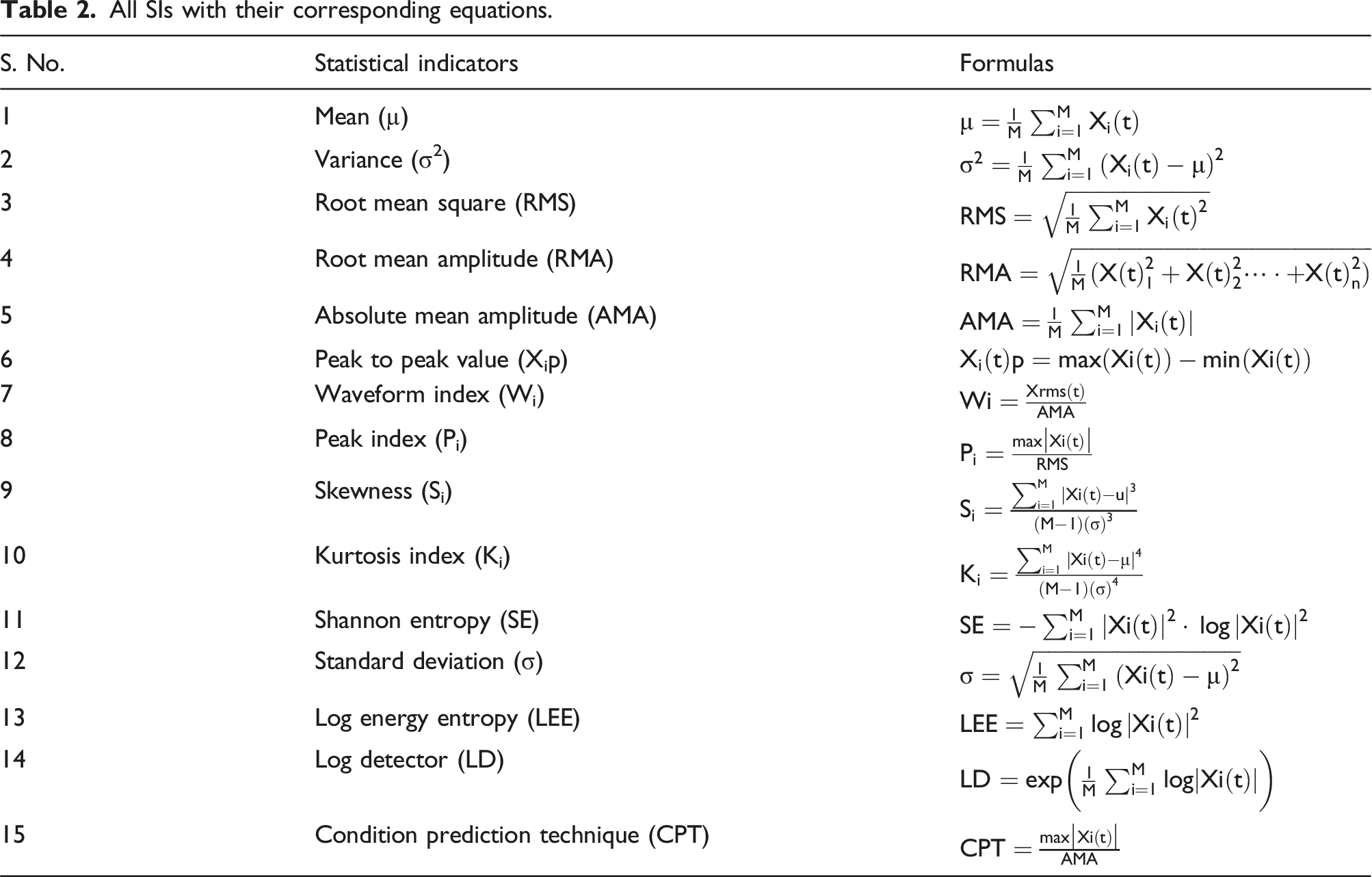
All SIs with their corresponding equations.
SIs of prominent PFs.
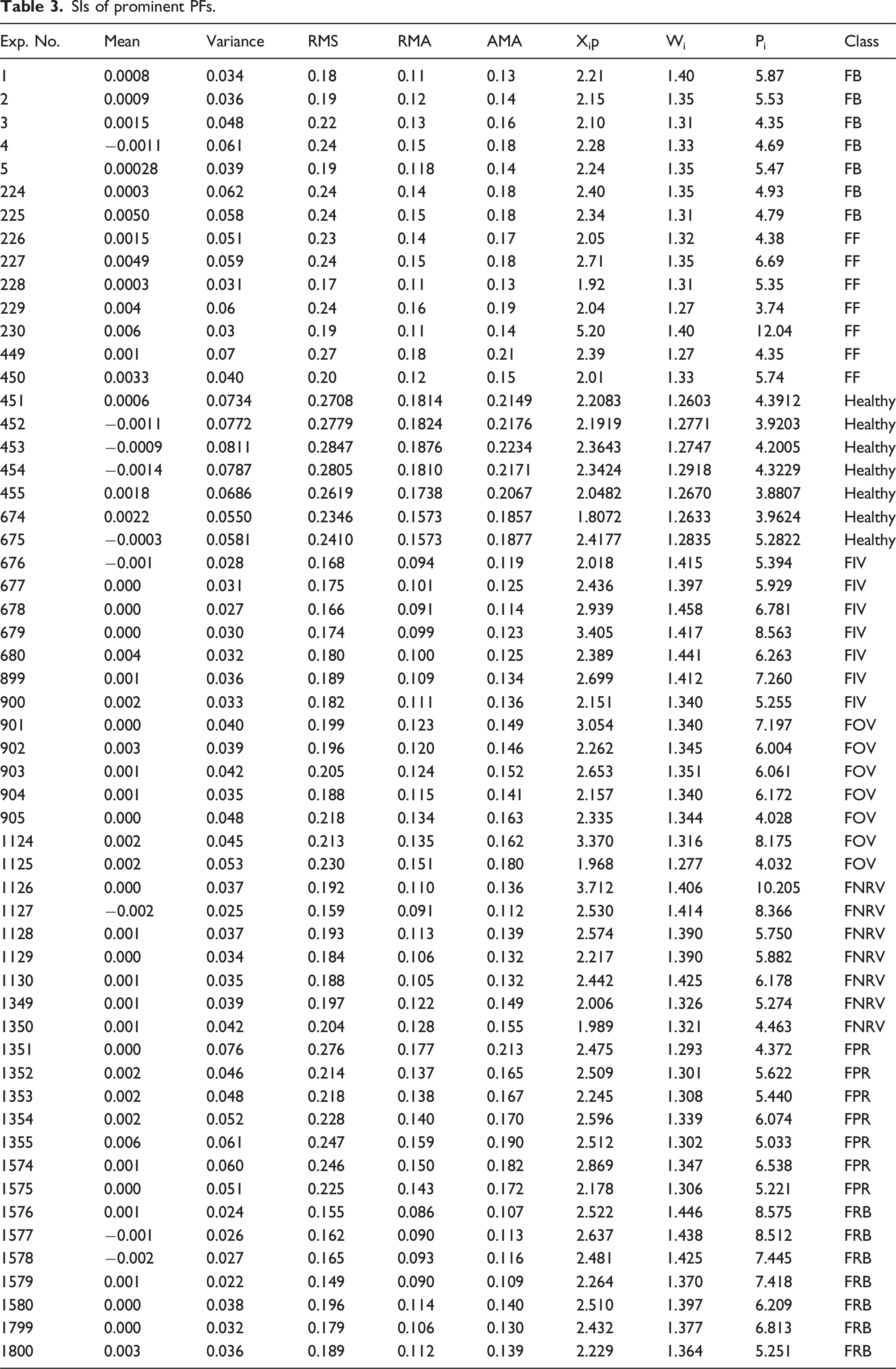
SIs of prominent PFs.

The statistical parameters for all 1800 data points were computed and are presented in Tables 3 and 4. These values were then analysed to identify the most appropriate statistical indicator for fault detection in an RAC setup. The plots of 15th statistical indicators against the sample size are shown in Figures 9 and 10. Upon examination, it is evident that the Kurtosis plot exhibits clearly defined and higher peaks compared to the other 14 SIs. Therefore, it can be concluded that Kurtosis is the most effective indicator for fault identification in an AC system. Statistical indicators versus samples graph. Statistical indicators versus samples graph.

Fault identification through kurtosis index-based B-cloud analysis
The primary objective of this study is to identify the critical state among the seven faulty conditions: Faulty Bearing (FB), Faulty Flywheel (FF), Faulty Inlet Valve (FIV), Faulty Outlet Valve (FOV), Faulty Nonreturn Valve (FNRV), Faulty Piston Ring (FPR), and Faulty Rider Belt (FRB). Kurtosis is a statistical measure that describes the shape of a signal’s distribution, particularly its peak. Signals with leptokurtic distributions have a relatively high and sharp peak, indicating more frequent extreme values. Platykurtic signals have a flatter top, with fewer extreme values and a more even distribution. Mesokurtic signals have a distribution that is neither too peaked nor too flat, resembling a normal distribution.
Figures 11–18 show kurtosis index-based bubble cloud analysis diagrams for the normal (healthy) and seven faulty conditions of the AC system. These figures represent the kurtosis index values using three different sizes of bubble clouds: large, medium, and small. The Kurtosis values for the large, medium, and small bubbles under the FB condition of the AC system are shown in Figure 11. From this figure, it can be observed that the large bubble for the FB condition has the highest Kurtosis index value (56.3) of all the bubble cloud analysis diagrams. This indicates a signal with a relatively high peak, called leptokurtic (>3), suggesting a fault in the bearing condition. Kurtosis index-based BCA diagram of FB. Kurtosis index-based BCA diagram of FF. Kurtosis index-based BCA diagram of FIV. Kurtosis index-based BCA diagram of FOV. Kurtosis index-based BCA diagram of FNRV. Kurtosis index-based BCA diagram of FPR. Kurtosis index-based BCA diagram of FRB. Kurtosis index-based BCA diagram of normal (healthy).


Figure 12, represents the kurtosis index values for FF, which vary from 3.34 to 35.9 (min. to max.). From this figure, it can be observed that the size of the bubble cloud for the FF condition is greater than 3 (called leptokurtic). This indicates a signal with a high peak, which suggests a fault in the flywheel condition.
Figure 13, represents the kurtosis index values for FIV, which vary from 4.2 to 17.5 (min. to max.). From this figure, it can be observed that the size of bubble cloud for the FIV condition is greater than 3 (called leptokurtic). This indicates a signal with a high peak, which suggests a fault in the inlet valve condition.
Figure 14, the kurtosis index values for FOV, which vary from 3.3 to 12.1 (min. to max.). From this figure, it can be observed that the size of bubble cloud for the FOV condition is greater than 3 (called leptokurtic). This indicates a signal with a high peak, which suggests a fault in the outlet valve condition.
Figure 15, represents the kurtosis index values for FNRV, which vary from 3.3 to 27.5 (min. to max.). From this figure, it can be observed that the size of bubble cloud for the FNRV condition is greater than 3 (called leptokurtic). This indicates a signal with a high peak, which suggests a fault in the non-return valve condition.
Figure 16, represents the kurtosis index values for FPR, which vary from 3.1 to 12.1 (min. to max.). From this figure, it can be observed that the size of bubble cloud for the FPR condition is greater than 3 (called leptokurtic). This indicates a signal with a high peak, which suggests a fault in the piston ring condition.
Figure 17, represents the kurtosis index values for FRB, which vary from 3.3 to 16.9 (min. to max.). From this figure, it can be observed that the size of bubble cloud for the FRB condition is greater than 3 (called leptokurtic). This indicates a signal with a high peak, which suggests a fault in the rider belt condition.
Figure 18, represents the kurtosis index values for normal (healthy) condition, which vary from 1.2 to 3.7 (min. to max.). From this figure, it can be observed that the size of bubble cloud for the normal (healthy) condition falls within the moderate (3) range (called mesokurtic). This indicates a signal with a moderate peak, suggesting that there is no fault in this state.
Summy of faults identification.

Classification using linear and quadratic discriminant analysis (LDA & QDA)
Classification using linear discriminant analysis (LDA)
LDA is a supervised machine learning technique used primarily for classifica-tion and dimensionality reduction. The goal of LDA is to find a linear combination of features that best separates two or more classes. This is achieved by maximizing the between-class variance and minimizing the with-in-class variance. The core mathematical foundations of LDA are as follows:
Step 1 - Problem setup
Suppose you have a dataset with n observations, each with p features, and belonging to one of K classes.
The dataset matrix,
The vector of class labels, where each entry corresponds to the class of the corresponding sample.
C k represents the kth class, and n k is the number of samples in class C k . μ k represents the mean of class Ck, and μ is the overall mean of the entire dataset.
Step 2 - Scatter matrices
LDA is based on two key scatter matrices that measure the spread of the data: • Within – class scatter matrices S
w
The within-class scatter matrix quantifies the variance within each class. It measures how much the samples within each class deviate from their respective class means.
The formula for the within-class scatter matrix SW,
Alternatively, can express S
W
as, • Between-class scatter matrix S
B


The between-class scatter matrix quantifies the variance between the different class means. It measures how much the class means deviates from the overall mean of all samples. The formula for the between-class scatter matrix S
B
,
The overall mean μ is computed as the average of all the class means,
Step 3 - The LDA objective
The primary objective of LDA is to find a projection that maximizes the separability between classes. This separability is measured as the ratio of the between-class scatter to the within-class scatter. The criterion function we want to maximize is:
Step 4 - Maximizing the criterion
To maximize J(w), we take the derivative with respect to w, w and set it equal to zero,
This results in the eigenvalue problem:
Step 5 - Finding the optimal projection
To find the best projection: • Solve the eigenvalue problem • The eigenvectors w
1
, w
2
… are ordered by their eigenvalues λ
1
, λ
2
, … • Select the top k −1 eigenvectors corresponding to the largest eigenvalues (where k is the number of classes). These eigenvectors define the new subspace for projection.

Step 6 - Dimensionality reduction
LDA typically reduces the data to K−1 dimensions, because there can be at most K−1 linearly independent directions of maximum class separability. In practice: • If K = 2, you reduce the data to 1D • If K = 3, you reduce the data to 2D • And so on.
Once the eigenvectors are determined, the data is projected onto the subspace spanned by the top K−1 eigen-vectors.
Classification using quadratic discriminant analysis (QDA)
QDA is a supervised machine learning technique used for classification. It is a generalization of LDA that allows for more flexibility by modeling each class with a separate covariance matrix. As a result, QDA can handle situations where the decision boundaries between classes are non-linear. The Mathematical foundation of QDA is as follows:
Given an observation x∈R d , we want to classify it into one of K classes. QDA computes the probability of each class, P (y = k∣x), and assigns the observation to the class with the highest probability.
Step 1 - Class conditional probability
For class k, assuming x is normally distributed with mean vector μ
k
and covariance matrix Σk, the likelihood P (x∣y = k) is given by the multivariate normal distribution: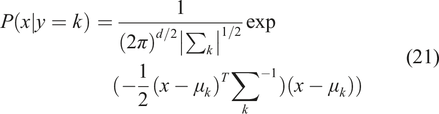
Step 2 - Bayes’ theorem
To classify an observation, we apply Bayes’ theorem to compute the posterior probability of class given the observation x,

Substituting the Gaussian likelihood,
Step 3 - Decision rule
The decision rule is to assign the class k that maximizes P(y = k|x), which simplifies to,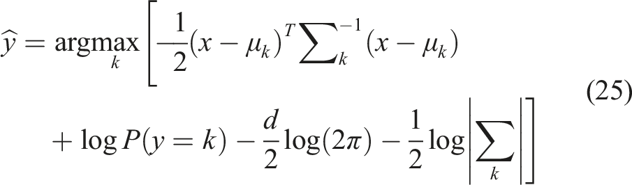
This is a quadratic decision boundary because the quadratic term comes from the term involving 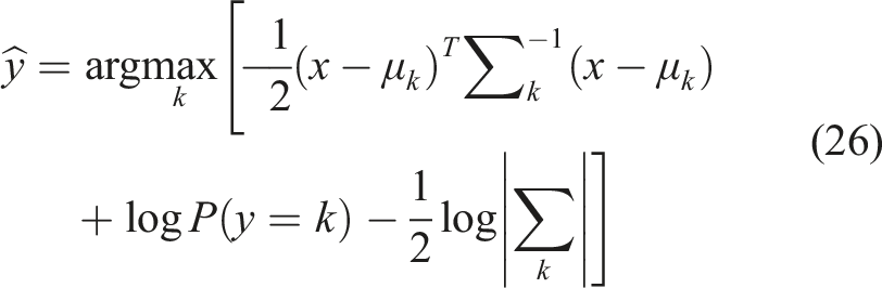
Step 4 - Quadratic discriminant
The term
Diagnosing of faults
In this study, features of the Faulty Bearing (FB) condition in the AC system have been identified through comparison with the normal condition. A total of 450 datasets, consisting of 225 datasets for both the normal and FB conditions, were divided in an 80:20 ratio. Figure 19 provides a detailed overview of the entire dataset. Summary of dataset.
This study utilizes linear and quadratic discriminant analysis for fault diagnosis. The analytical results are presented using three methods: Scatter Plot (SP), Confusion Matrix (C-Matrix), and Receiver Operating Characteristic (ROC) curves.
Fault diagnosis using scatter plot (SP)
The relationship between the two classes in the dataset is vividly illustrated through the scatter plot (SP). As shown in Figure 20, the classification results are represented in the SP, where samples are plotted against their kurtosis values for both normal and faulty bearing conditions. In this plot, blue circles represent the normal (healthy) state, while red circles indicate the faulty state. The red circles show a significantly disrupted distribution, referred to as Leptokurtic, which indicates a signal with a relatively high peak, suggesting a faulty bearing case. Conversely, the blue samples represent a stable state known as Platykurtic, characterized by a flat-topped signal that implies the absence of a fault. SP of FB and normal condition.
Fault diagnosis using confusion matrix (C-matrix)
The C-Matrix is a table that shows how well an algorithm can classify data by predicting a categorical label for each instance of input. As shown in Figure 21, it displays true positive (TP), true negative (TN), false positive (FP), and false negative (FN) values, determined by the test data and model. This matrix is used to evaluate the predictive effectiveness of the classification method in the current study. C-matrix.
In the current study, both LDA and QDA were employed to diagnose faults. The confusion matrix for LDA and QDA considers both normal and faulty bearing (FB) conditions in the AC system, as shown in Figures 22 and 23. This matrix is used for assessment and provides statistics for true positives (TP), true negatives (TN), false positives (FP), and false negatives (FN) in both training and testing scenarios. These parameters contribute to the overall classification accuracy of LDA and QDA, and the performance of the methods is described in detail below. C-matrix of LDA. C-matrix of QDA.

Fault diagnosis using ROC curves
The true positive rate (TPR) and false positive rate (FPR) of the LDA and QDA predictive abilities for fault detection in the AC system are evaluated using ROC curves. In these curves, a red dot signifies the classifier’s performance, representing the values of TPR and FPR.
Fault diagnosis using ROC curves with LDA
For the training cases, the LDA is shown to allocate values sequentially based on false positive rates (FPR) of 0.12 and 0.10 in Figure 24(a) and (b), indicating that 12% and 10% of the values are incorrectly assigned to the positive class, respectively. For the testing cases, the LDA allocates values sequentially based on FPR of 0.21 and 0.12 in Figure 24(c) and (d), showing that 21% and 12% of the values, respectively, are incorrectly categorized as belonging to the positive class. ROC curves of LDA.
The TPR values of 0.90 and 0.88 indicate that the LDA successfully identifies 90% of the normal class and 88% of the faulty bearing (FB) class as positive during the training phase. In the testing phase, TPR values of 0.88 and 0.79 show that the classifier accurately classifies 88% of the normal class and 79% of the FB class as positive.
Fault diagnosis using ROC curves with QDA
For the training cases, the QDA is shown to allocate values sequentially based on false positive rates (FPR) of 0.25 and 0.05 in Figure 25(a) and (b), indicating that 25% and 05% of the values are incorrectly assigned to the positive class, respectively. For the testing cases, the QDA allocates values sequentially based on FPR of 0.21 and 0.02 in Figure 25(c) and (d), showing that 21% and 02% of the values, respectively, are incorrectly categorized as belonging to the positive class. ROC curves of QDA.
The TPR values of 0.95 and 0.75 indicate that the LDA successfully identifies 95% of the normal class and 75% of the faulty bearing class as positive during the training phase. In the testing phase, TPR values of 0.98 and 0.79 show that the classifier accurately classifies 98% of the normal class and 79% of the FB class as positive.
Result and accuracy of LDA and QDA
In this research, the performance of the LDA and QDA are assessed in terms of accuracy. Classifier accuracy is defined as the proportion of correct predictions to the total number of input samples.
Accuracy of LDA
The values for TP, TN, FP, and FN of training case for the LDA are 159, 161, 18, and 22, respectively, as illustrated in Figure 22(a).

Accuracy of QDA
The values for TP, TN, FP, and FN of testing case for the QDA are 168, 09, 45, and 138, respectively, as illustrated in Figure 23(a).

Conclusions
This study presents an effective and comprehensive methodology for identifying and predicting faults in air compressor (AC) systems using advanced signal processing and discriminant-analysis-based machine learning techniques. The experimental analysis demonstrates several important findings. First, the Local Mean Decomposition (LMD) technique proved significantly more effective than Empirical Mode Decomposition (EMD) for processing AC acoustic signals. LMD offered superior separation of frequency components and minimized mode mixing, resulting in clearer fault-related information. Second, among the 15 statistical indicators evaluated, the kurtosis index emerged as the most reliable feature for fault characterization. Its integration with the Bubble Cloud (B-Cloud) analysis technique enabled the accurate identification of fault signatures across different AC components. Faulty flywheel (FF) and faulty bearing (FB) conditions exhibited the highest kurtosis index values (56.3 and 35.9, respectively), indicating that the bearing fault produces more prominent vibration disturbances compared to other faulty states. Third, the classification performance of discriminant-analysis-based machine learning algorithms revealed that Linear Discriminant Analysis (LDA) outperformed Quadratic Discriminant Analysis (QDA). LDA achieved the highest prediction accuracy of 88.88%, establishing it as the most suitable classifier for fault detection in this study.
Overall, the proposed methodology which combines LMD, statistical indicators, kurtosis-based B-Cloud analysis, and LDA offers a robust and accurate approach for identifying and predicting in-situ fault features in real-time air compressor systems. This approach can significantly enhance the reliability, safety, and predictive maintenance capabilities of AC installations in industrial applications.
Footnotes
Declaration of conflicting interests
The authors declared no potential conflicts of interest with respect to the research, authorship, and/or publication of this article.
Funding
The authors received no financial support for the research, authorship, and/or publication of this article.

Data Availability Statement
Data will be made available upon request.