There is no significant trend in global average temperature

Abstract

The HadCRUT4 time series of 166 annual values of global average temperature was analysed both deterministically and stochastically and the results compared. The deterministic model comprised the sum of a linear trend and a multi-decadal oscillation fitted by ordinary least squares regression. The stochastic model was an ARMA(1,2) model with a drift term included. The deterministic model showed a linear trend of 0.5℃ per century while the stochastic model showed no significant drift. In both cases, the residuals were tested for self-correlation using standard statistical tests. The residuals from the deterministic model were significantly self-correlated whereas those from the stochastic model were not. We conclude that the stochastic model was a much better fit to the data and that the apparent linear trend of the deterministic model was spurious and a consequence of performing a regression in which time was the explanatory variable.

Keywords

Global average temperature trend deterministic stochastic false drift spurious regression centrally biased random walk red spectra

Introduction

In recent decades, energy policy, both nationally and internationally, has been primarily concerned with the reduction in carbon emissions from the combustion of fossil fuels. This has arisen from a proliferation of theories of climate, encapsulated in complex numerical models, which purport to relate global surface air temperature to the concentration of carbon dioxide in the atmosphere. All this activity is based on a single empirical observation, viz. that there has been a significant increase in global average temperature over the last century and a half. Here we show that this observation is false and is based on an overly-simplistic interpretation of the data.

Discussion

In physics, there are a number of important dichotomies. These include the dichotomy between relativistic and Newtonian mechanics, between quantum and classical field theories and between linear and non-linear systems. There is a further dichotomy, equally important, the dichotomy between deterministic and stochastic processes. It might be argued that this is mere sophistry with little practical consequence but that is not so. Indeed, the conclusion of this article that ‘the stochastic model was a much better fit to the [global average temperature] data’ indicates that systems which are as fundamentally stochastic as fluid dynamic systems must be treated statistically lest spurious alarms and costly false positives result.

A deterministic process is a process for which, once initial conditions are known, all future states of a system can be predicted. A stochastic process is a process for which, given the initial conditions, futures states are not completely predetermined but are governed by the laws of probability.

Any system describable in terms of analytic functions or differential equations alone is deterministic. The interaction of solid objects with force fields and with one another are well described by deterministic models. Celestial mechanics is an example.

Fluid dynamical systems are commonly dealt with deterministically using the Navier–Stokes equations or variations thereof. In order to do this, it is commonly assumed that the fluid involved is a ‘continuum’, i.e. it is everywhere continuous and differentiable and so is deterministic, as when the Navier–Stokes equations are converted to the discrete form of finite difference equations for the purpose of numerical modelling of fluids. Here Taylor’s theorem is commonly used to make the transition to the discrete case, the continuum assumption being implicit in this use of Taylor’s theorem.

It has been well known for more than a century that no real fluid is a true continuum. This is demonstrated by the Brownian motion. The velocity field in any real fluid varies rapidly and discontinuously in both time and space. It is not differentiable. Hence the use of Taylor’s theorem in defining the finite difference equations of numerical models is not justified. Instead, there is a probabilistic relationship between the state of a fluid and the preceding state. Real fluids are stochastic not deterministic. Observed fluid dynamic phenomena such as turbulence, vortex shedding and wave breaking are testament to the stochastic nature of real fluids. Even at laboratory scales, the Navier–Stokes equations cannot adequately describe the behaviour of fluids in high Reynold’s number regimes. Aspects of these regimes which can be quantified are dependent on other methods such as dimensional arguments, self-similarity and physical intuition. Kolmogorov’s turbulence spectrum is an example.

If a system is deterministic, then its variables are all single-valued functions of time. Experimental observations of dynamical variables are commonly displayed as functions of time and a ‘line of best fit’ or regression line fitted to the observations to display the trend or rate of change with time. This is commonplace, something most researchers learned at school.

However, there can be serious problems with this methodology when the system under investigation is stochastic. Nelson and Kang¹ demonstrated that, for certain stochastic processes such as a ‘random walk’, the use of time as the explanatory variable can lead to the appearance of a trend even though none was present in the original data. They report for a random walk process: Regression of a random walk on time by least squares will produce R² values of around .44 regardless of sample size when the variable has, in fact, no dependence whatever on time (zero drift). It follows that an observed trend obtained by regressing a physical quantity on the time may or may not be real, depending on the deterministic or stochastic nature of the system under investigation. Although not widely known outside the field of Econometrics, the implications of this article cannot be overestimated. It seems to be little known in the physical sciences.

Attempts to model global climate have hitherto depended on coupled ocean-atmosphere general circulation models. Such models are deterministic because the Navier–Stokes equations of fluid dynamics on which they are based are, themselves, deterministic.

Hasselmann² proposed a stochastic model of climate variability wherein slow changes in climate are explained as the integral response to continuous random excitation by short period ‘weather’ disturbances. Thus, intrinsic quantities such as temperature are the outcome of the integration by natural processes of quasi-random, extrinsic quantities such as heat. As a consequence, such measurements can be regarded as the outcome of a stochastic process and can be expected to exhibit a power law spectrum with negative exponent due to such integrating effects. The best known and simplest example of such a process is the ‘random walk’ obtained when white noise is integrated or summed. It has a power law spectrum with an index of −2.

Pelletier³ has shown that variance spectrum of atmospheric temperature exhibits a variety of power law relationships over a wide range of time scales from 2 years to 100,000 years, i.e. over a given frequency scale:

S = {Af}^{ν}

(1)

where S is the variance density at frequency, f, and A and ν are constants. Pelletier found that ν lay in the range −2.0 to −0.5 indicating a concentration of variance density at low frequencies, i.e. random-walk-like behaviour.

In recent times, much has been made of the apparent rising trend in global average temperature commonly attributed to rising greenhouse gas concentrations in the atmosphere. At issue is whether this trend is a real, deterministic trend or whether the observed variations are merely the random outcome of a stochastic process.

The data

Two time series were downloaded for analysis. They were:

The HadCRUT4 series of 1666 annual values from 1850 to 2015 inclusive were downloaded from http://www.metoffice.gov.uk/hadobs/hadcrut4/data/current/time_series/ on 12 April 2016.⁴ There are a number of such global temperature data sets available, e.g. those from GISS, NOAA and BEST. Statistically, they are almost identical. HadCRUT4 was chosen because it was longer.

A data set of proxy temperatures from isotope ratios in Greenland ice cores, the GISP2 Ice Core Temperature and Accumulation Data. These were downloaded from ftp://ftp.ncdc.noaa.gov/pub/data/paleo/icecore/greenland/summit/gisp2/isotopes/gisp2_temp_accum_alley2000.txt on 20 April 2016.^5,6 Like most ice core records, the data values were sampled at unequal intervals of time. In order to convert them to a form suitable for processing, the record was divided into 50-year intervals and the data averaged in each interval to form a time series. Only the most recent 10,000 years of ice core data were used, i.e. the data were all from the Holocene Epoch.

A deterministic model

A deterministic model typically comprises a linear function of one or more functions of the explanatory variable plus a random element. In this case, the explanatory variable is the time. The parameters are estimated by minimizing the sum of squares of the differences between an estimate and the true values of the sample, the residuals. This is the ordinary least squares (OLS) method. It is based on the assumption that a deterministic relationship with the explanatory variable does exist and that the random elements at different times have zero mean and are independent of one another. The random element can be thought of as ‘measurement error’.

The model

The HadCRUT4 time series values were fitted with a straight line by the OLS method of linear regression, i.e. the model

y_{t} = a_{0} + a_{1} t + ξ_{t}

(2)

was fitted to the data and is shown as the straight line in Figure 1(a).

Figure 1.

The deterministic method: (a) The HadCRUT time series. The straight solid line shows the linear trend of temperature vs. time. The dashed line shows the multiple regression fit of a linear trend plus a sinusoid. (b) Residuals from the time series of the linear trend plus sinusoid. (c) The autocorrelation function of the residuals, φ.

There is also the appearance of a ‘multi-decadal oscillation’ present so a regression model of the form

y_{t} = a_{0} + a_{1} t + a_{2} \cos (ω t) + a_{3} \sin (ω t) + ξ_{t}'

(3)

was also fitted. The angular frequency, ω, was chosen by trial and error and corresponded to a period of 70 years. The estimates

{\overset{\land}{a}}_{0}

{\overset{\land}{a}}_{1}

{\overset{\land}{a}}_{2}

and

{\overset{\land}{a}}_{3}

of the model parameters a₀, a₁, a₂ and a₃ are shown in Table 1.

Table 1.

Coefficient estimates for the deterministic model of equation (3).

	Value	Std err	t	p > \|t\|	95.0% Conf. int.
${\overset{\land}{a}}_{0}$	−0.0149	0.010	−1.508	0.134	−0.035, 0.005
${\overset{\land}{a}}_{1}$	0.0050	0.000	24.394	0.000	0.005, 0.005
${\overset{\land}{a}}_{2}$	0.1210	0.014	8.841	0.000	0.094, 0.148
${\overset{\land}{a}}_{3}$	0.0791	0.014	5.569	0.000	0.051, 0.107

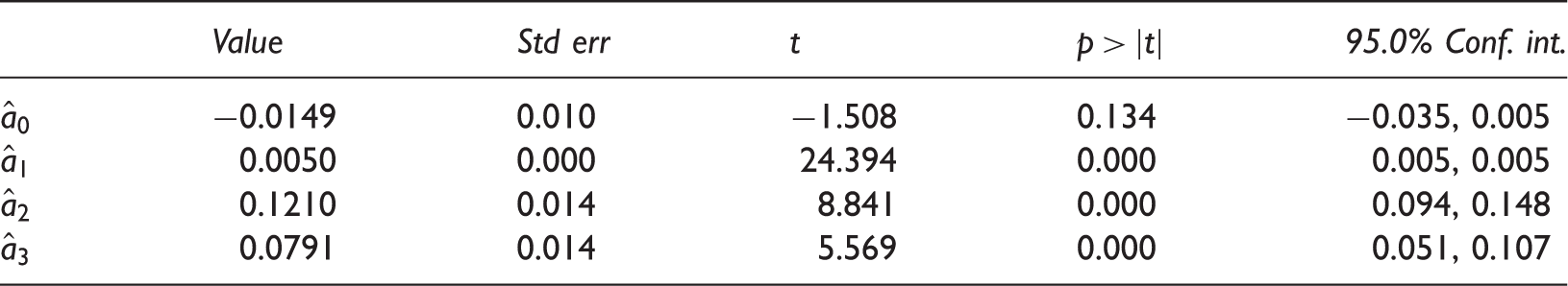
Standard error, t-value, p-value and 95% confidence intervals are shown for each.

The fitted function (dashed curve) described by (2) is shown superimposed on the data in Figure 1(a). The linear trend in temperature, if it is real, is given by coefficient estimate, ${\overset{\land}{a}}_{1}$ , i.e. half a degree Celsius per century.

Testing the fit of the deterministic model

The fitting of a function by OLS regression requires that the sequence of residuals ${ξ_{t}}$ in (2) or ${ξ'_{t}}$ in (3) be unselfcorrelated. Clearly that is not the case for (2) where a sinusoidal function or ‘multi-decadal oscillation’ would remain after removal of the linear trend. For this reason, a sinusoid of arbitrary phase was included in the model of equation (3).

The sequence of residuals,

{ξ'_{t}}

, is shown in Figure 1(b) and its autocorrelation function (ACF) in Figure 1(c). Even to the naked eye, there appears to be a systematic positive trend in the ACF out to Lag 30. There are two statistical tests, which can be used to determine whether the non-zero values of the ACF at non-zero lags are significant or just due to chance. These are the Breusch–Godfrey test^7,8 and the Ljung–Box test.⁹ The results obtained when these tests were applied to the fitting of equation (3) to the HadCRUT4 data are shown in Table 2.

Table 2.

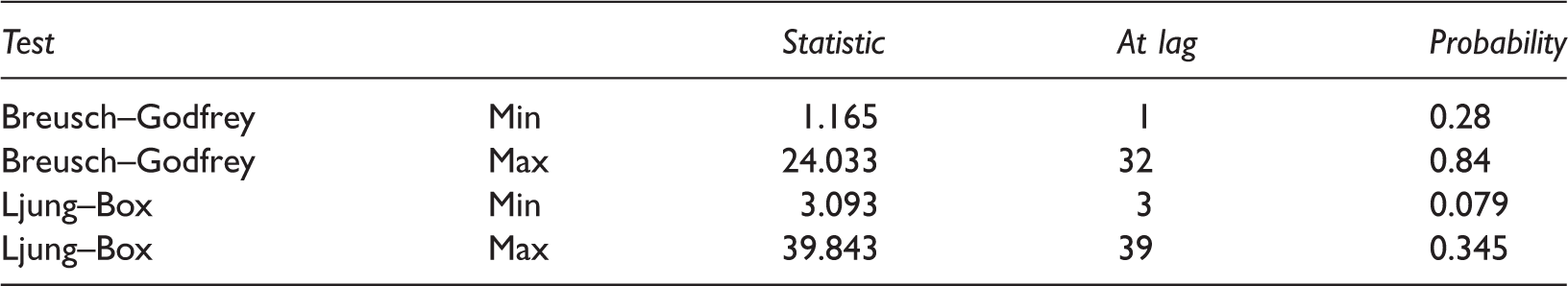
Testing the residuals of regression model of equation (3) for self-correlation.

Test		Statistic	At lag	Probability
Breusch–Godfrey	Min	52.023	1	5.487 × 10⁻¹³
Breusch–Godfrey	Max	73.120	36	2.498 × 10⁻⁴
Ljung–Box	Min	92.665	3	0
Ljung–Box	Max	232.052	39	0

Minimum and maximum values of the Breusch–Godfrey and Ljung–Box test statistics and their corresponding probabilities for a maximum lag of 40.

The probabilities listed in Table 2 are so small that we can reject the null hypothesis that the non-zero ACF values are purely random and that equation (3) is a good fit to the data. It can be rejected at a very high level of significance.

The stochastic model

A stochastic model is based in the assumption that the value at any given time is deterministically related to the value or values at p previous times plus an additional random element. When the random elements are independently distributed the model is known as an ‘autoregressive’ (AR) model of order p.

The random element may itself be a linear function of q independent random variables each with zero mean in which case the model is said to have a ‘moving average’ (MA) component of order q. Combining the two gives an autoregressive moving average model of order (p, q), an ARMA(p, q) model.

The random components are not regarded as measurement errors but as properties inherent in the system itself.

The model

An ARMA(1,2) model was fitted to the HadCRUT4 time series using the Python statistical package: statsmodels.tsa.arima-model.ARMA. The package’s css-mle option was selected whereby the conditional sum of squares likelihood was maximized and its values used as starting values for the computation of the exact likelihood via a Kalman filter.

The fitted model was thus

y_{t} = a_{1} y_{t - 1} + ε_{t} + b_{1} ε_{t - 1} + b_{2} ε_{t - 2} + c

(4)

where a₁, b₁, b₂ and c were parameters to be fitted and the

{ε_{t}}

were independent, identically distributed random variables with zero mean. The orders, p = 1 and q = 2, were found by trial and error, i.e. as the smallest values which resulted in unselfcorrelated residuals.

Note that the parameter c is similar to the coefficient a₁ in (2) and (3). Setting a₁ = 1 and the other coefficients in (4) to zero for the moment, gives

y_{t} = y_{t - n} + nc

(5)

so that y_t becomes a deterministic linear function of the elapsed time,

n Δ t

. For this reason, c is known as the ‘drift term’. It is a deterministic element in an otherwise stochastic model.

The estimates

\overset{\land}{a_{1}}, \overset{\land}{b_{1}}, \overset{\land}{b_{2}}

and

\overset{\land}{c}

of the model parameters

a_{1}, b_{1}, b_{2}

and c are shown in Table 3.

Table 3.

Coefficient estimates for the stochastic model of equation (4).

	Coef.	Std. err.	z	p > \|z\|	95% Conf. int.
${\overset{\land}{a}}_{1}$	0.9955	0.006	176.629	0.000	0.984, 1.007
${\overset{\land}{b}}_{1}$	−0.4068	0.074	−5.490	0.000	−0.552, −0.262
${\overset{\land}{b}}_{2}$	−0.2276	0.067	−3.379	0.001	−0.360, −0.096
$\overset{\land}{c}$	0.0736	0.351	0.210	0.834	−0.615, 0.762

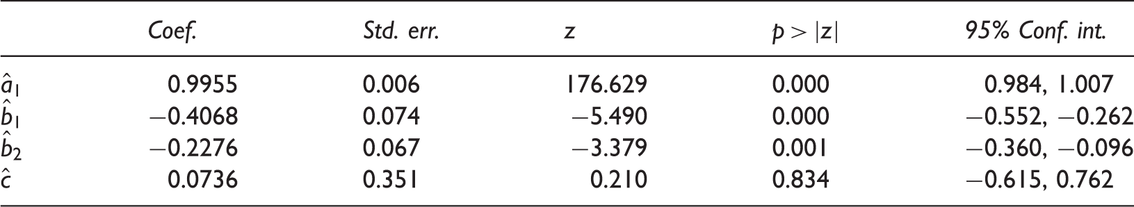
Standard error, z-value, p-value and confidence limits are shown for each.

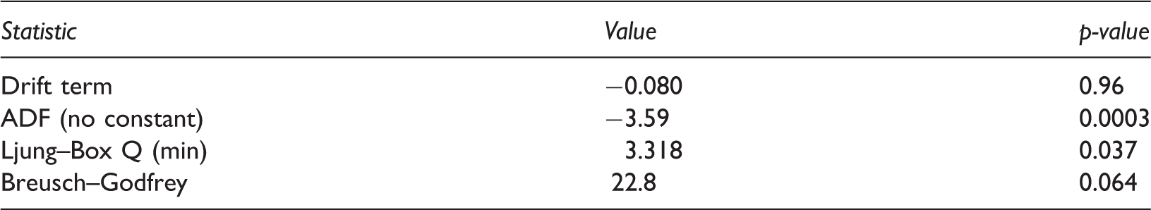
The most important feature of Table 3 is the small value and large confidence interval of the drift term estimate, $\overset{\land}{c}$ . It is not significantly different from zero. Unlike the deterministic model, stochastic modelling indicates that there is no significant drift in the HadCRUT4 time series of global average temperature.

Also of interest is the autoregressive coefficient, ${\overset{\land}{a}}_{1}$ , which is very close to one. This is important because, were the population value, a₁, to be equal to one then the time series would be a true random walk and so non-stationary. This issue is discussed further below.

Testing the fit of the stochastic model

The sequence of residuals is shown in Figure 2(b) and its autocorrelation function in Figure 2(c). The ACF values at non-zero lags appear to be randomly distributed on either side of zero. As before the Breusch–Godfrey test and Ljung–Box tests were used to see if the null hypothesis that the residual are unselfcorrelated can be rejected. The results are shown in Table 4. None of the probabilities listed in Table 4 lie below the critical value of 0.05 and so there is no reason to reject the null hypothesis that the non-zero value of the ACF are due entirely to chance. The ARMA(1,2) model is a very good fit to the HadCRUT4 time series.

Figure 2.

The stochastic method: (a) The HadCRUT time series. (b) Residuals from fitting an ARMA(1,2) model, (c) The autocorrelation function of the residuals, φ.

Table 4.

Testing the residuals of the ARMA(1,2) model for self-correlation.

Test		Statistic	At lag	Probability
Breusch–Godfrey	Min	1.165	1	0.28
Breusch–Godfrey	Max	24.033	32	0.84
Ljung–Box	Min	3.093	3	0.079
Ljung–Box	Max	39.843	39	0.345

Minimum and maximum values of the Breusch–Godfrey and Ljung–Box test statistics and their corresponding probabilities for a maximum lag of 40.

The frequency domain

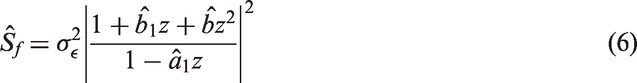
Whereas a deterministic model such as (3) can be displayed in the time domain, as in Figure 1(a), it is usually more useful to display stochastic models in the frequency domain as variance density spectra. The ARMA parameters allow the population variance spectral density, S_f, of the time series to be estimated as a continuous function of the frequency, e.g. for the ARMA(1,2) process discussed here:

{\overset{\land}{S}}_{f} = σ_{ε}^{2} | \frac{1 + {\overset{\land}{b}}_{1} z + \overset{\land}{b} z^{2}}{1 - {\overset{\land}{a}}_{1} z} |^{2}

(6)

where

z = \exp (2 π if Δ t)

(7)

Δ t

is the sampling interval and

σ_{ε}^{2}

is the variance of the residuals.

The HadCRUT4 time series

Figure 3 shows the ARMA(1,2) spectral estimate of the HadCRUT4 time series plotted using logarithmic scales (thick line). Also shown is the periodogram of the sample (thin line).

Figure 3.

The variance density spectral estimate, ${\overset{\land}{S}}_{f}$ , vs. frequency, f of the ARMA(1,2) model fitted to the HadCRUT time series (thick line). The thin line shows the periodogram of the time series. The vertical-dashed line shows $f_{3 dB}$ , the 3 dB cut-off frequency.

As a consequence of the above-discussed whiteness tests confirming the absence of self-correlation of the residuals, this spectral estimate is optimal. There can be no peak, trough or trend in the spectrum other than those depicted in Figure 2, because this would require further poles and/or zeros in the z-plane, which are not included in the ARMA model. Such extra poles or zeros, if unaccounted for, would inevitably lead to self-correlation of the residuals, which would then have failed the Ljung–Box and Breusch–Godfrey tests.

For $a_{1} = 1$ , there is a singularity in S_f in (6) at zero frequency. When $a_{1} \neq 1$ , the spectrum at low frequencies is flattened. In electronic terms, the spectrum resembles that of low-pass filtered white noise with a 3 dB cutoff given by

f_{3 dB} = \frac{1 - {\overset{\land}{a}}_{1}}{2 π Δ t}

(8)

where a₁ is the estimate of the autoregressive coefficient listed in Table 3 and

Δ t

is the sampling frequency. It is depicted as the vertical-dashed line in Figure 3 at

f_{3 dB} = . 00071

corresponding to a period,

T_{3 dB} = 1400

years.

The $a_{1} = 1$ case is extremely important statistically. The singularity means that the variance density at the origin is not defined. In the time domain, we would have a true random walk for which variance is proportional to elapsed time and the time series cannot be assumed to be stationary. There is a statistical test, the Augmented Dickey–Fuller (ADF) test, which tests the null hypothesis of whether a unit root is present in a time series sample. The HadCRUT4 time series in question yielded an ADF statistic of −0.3011 with a p-value of 0.576. Hence, the null hypothesis cannot be rejected. It is possible that there is a unit pole, i.e. that $a_{1} = 1$ .

Of course, this does not imply that a unit pole exists, only that its existence cannot be rejected. In the field of Econometrics, such a result would sound an alarm and the researcher would be tempted to abandon the ARMA model for an ARIMA model appropriate to a non-stationary time series.

However, examination of Figure 3 shows that the 3 dB cutoff frequency is much smaller than the smallest frequency in the periodogram, i.e. the cutoff period of 1400 years is much longer than the sample length of 166 years. By using the ADF test to determine whether the time series is non-stationary, we are attempting to predict behaviour of the spectrum for periods which are an order of magnitude greater than the sample length. Common sense would suggest that this is unreliable.

The GISP2 time series

Casting further light on this issue requires a much longer time series. Although the length of contemporary time series was limited by the short period during which accurate temperature measurements were made, subsidiary data are available in the form of proxy temperature time series derived from stable isotope ratios of atmospheric gases trapped in ice-cores. There is a trade-off between length of such proxy records and their time resolution. At longer time scales, events such as ice-age terminations suggest an underlying quasi-deterministic process which depends on astronomical quantities¹⁰ and which cannot be assumed to be stationary. It is therefore desirable to use data from the relatively recent past, the Holocene epoch of the last 10,000 years following the last Ice Age Termination.

The GISP2 proxy-temperature time series fom Central Greenland ice cores was such a data set with a time resolution of 50 years over the last 10,000 years. A time series of equally spaced values was constructed from the GISP2 data by averaging the value in each 50-year interval. It is displayed in Figure 4(a).

Figure 4.

(a) Time series of the GISP2 Central Greenland ice-core proxy temperature anomaly for the last 10,000 years. (b) The population spectrum of the fitted ARMA(1,3) process (thick line) and periodogram (thin line) of this time series shown in (a). The vertical-dashed line shows $f_{3 dB}$ , the 3 dB cut-off frequency.

An ARMA(1,3) process was fitted to this time series and its spectral estimate and periodogram are shown in Figure 4(b). The various goodness-of-fit statistics are shown in Table 5.

Table 5.

Statistics of the GISP2 time series.

Statistic	Value	p-value
Drift term	−0.080	0.96
ADF (no constant)	−3.59	0.0003
Ljung–Box Q (min)	3.318	0.037
Breusch–Godfrey	22.8	0.064

A striking difference from the HadCRUT spectrum is the existence of a strong trough with a minimum at .0045 year⁻¹ (period = 223 years). While spectral peaks display the presence of deterministic cycles or resonant phenomena, a trough such as this one implies a convoluting or averaging process. A possible explanation lies in the diffusion of atmospheric gases between layers during the firn stage of ice formation, an unavoidable artefact of the ice core proxy-temperature methodology.

A summary of the statistics is shown in Table 5. Once again the drift term is not significant, but this time, the ADF test indicates that we can dismiss the null-hypothesis that the time series has a unit pole with a high degree of confidence. This time the low pass cut-off is at $f_{3 dB} = . 000847$ year⁻¹, i.e. a period of 1180 years, well within the 10,000 year time span of the data and remarkably close to the 1400 year cut-off of the HadCRUT4 data.

This evidence from proxy data suggests that the contemporary HadCRUT4 time-series may well be stationary and not a true random-walk.

Demonstrating false correlation with a synthetic time series

If the HadCRUT4 time series of global average temperature is not a true random walk, it is important to determine whether Nelson and Kang’s conclusions still applies: is a false correlation with time possible when the series is stationary? For that purpose, a number of simulations were run for time series generated artificially using the parameters listed in Table 3 and with the drift term, c, set to zero. Each synthetic time series was 166-long and generated by the process:

y_{t} = {\overset{\land}{a}}_{1} y_{t - 1} + ε_{t} + {\overset{\land}{b}}_{1} ε_{t - 1} + {\overset{\land}{b}}_{2} ε_{t - 2}, t = 3, 4, \dots,, 168

(9)

where y₂ was set to zero and the

{ε_{t}}

where independent normally distributed random numbers.One million time series samples were generated in this way.

For each sample, r, the correlation coefficient of y_t on t was calculated and the number of values in each percentage binned to give the frequency distribution, f. The outcome is plotted in Figure 5. The distribution is bi-modal with peaks near $\pm 0.70$ demonstrating that not only it is possible to obtain a numerically large correlation coefficient of value on time but also it is likely. This is true, not only for random walk data described by Nelson and Kang, it is also true for the stationary ARMA(1,2) time series described here.

Figure 5.

The frequency, f, of r, the sample correlation coefficient holding between value and time for one million 166-long samples generated by equation (9).

The reason for this behaviour is demonstrated graphically in Figure 6. A single 10,000-long time series was also generated using equation (9) and is shown in Figure 6(a). Thus, Figures 4(a) and 6(a) are directly comparable. The former looks smoother because of the spectral trough at .0045 year⁻¹ attributable to firn processes. Figure 6(a) shows the time series we would expect to see if we had 10,000 years of global average temperature data rather than only 166 years.

Figure 6.

(a) A 10,000 long-time series of ‘annual temperatures’ generated artificially using the coefficients of the ARMA(1,2) model of Figure 2 and filtered and decimated in the same manner as the GISP2 data shown in Figure 4(a). (b) A 166-long segment showing the detail between the vertical lines in (a).

The two dashed vertical lines in Figure 6(a) designate an arbitrarily located 166-year long interval. The detail of the interval, expanded in time, is displayed in Figure 6(b). It exhibits an upward ‘trend’ remarkably similar to that of the HadCRUT4 data. There are many other 166-long intervals in Figure 6(a), which would have given a similar result and many others which would have shown an apparent downward trend.

It is clear from Figure 6 that such spurious upward and downward trends occur in a short sample of a time series when there is a large concentration of variance at periods longer than sample length, i.e. when the time series has a ‘red’ spectrum. This is still true even when the spectrum is flattened at low frequencies providing the 3 dB cut-off period is much longer than the sample length, i.e. when

T_{3 dB} >> N Δ t

(10)

where N is the sample length and

Δ t

is the sampling period. It is not necessary that the time series be a true random-walk and be non-stationary as is commonly believed.

Note also that a ‘multi-decadal oscillation’ appears in Figure 6(b). It is as spurious as the rising trend since no oscillatory behaviour is implied by the generating equation (10).

Conclusion

The process which gives rise to a red spectrum flattened below a cut-off frequency is widely found in engineering and in nature. In electronics, it occurs when electronic noise is fed through an RC integrator as with the bass control of an audio amplifier. In the natural world, it occurs when energy is randomly stored. It is a particular sort of Markov process termed a ‘centrally biased random walk’ and known colloquially as ‘red noise’. Using the techniques described above other ‘oscillations’ such as the Pacific Decade Oscillation can also be shown to be centrally biased random walks specified by a small number of ARMA parameters. This is not surprising since the PDO is derived from a large subset of the global average temperature data used here.

The small increase in global average temperature observed over the last 166 years is the random variation of a centrally biased random walk. It is a red noise fluctuation. It is not significant, it is not a trend and it is not likely to continue.

Footnotes

Declaration of conflicting interests

The author(s) declared no potential conflicts of interest with respect to the research, authorship, and/or publication of this article.

Funding

The author(s) received no financial support for the research, authorship, and/or publication of this article.

John Reid was awarded a PhD by the University of Tasmania in 1973 for his discovery of cosmic noise absorption pulsations in the auroral zone ionosphere. This work also accounted for the origin of “Pi1” micropulsations and remains the accepted explanation of this phenomenon. As a physicist with the Australian Antarctic Division, he became interested in statistical methods for extracting optimal information from noisy geophysical data and, later, in its application to speech recognition. With CSIRO's Division of Oceanography, he collected and analyzed ocean wave data from Tasmania's West Coast and developed a theory to account for frequency downshifting in wind-seas. He went on to form a company to develop a patent for video motion detection in surveillance applications. He is a “jobbing physicist”, a generalist, with a strong interest in the application of statistics to real world data. He and his wife, Rosie, live near Cygnet in Southern Tasmania.

References

Nelson

Kang

. Pitfalls in the use of time as an explanatory variable in regression. J Business Econom Stat 1984; 2: 73–82.

Hasselmann

. Stochastic climate models. Part I. Theory. Tellus 1976; XXVIII: 473–485.

Pelletier

. Natural variability of atmospheric temperatures and geomagnetic intensity over a wide range of time scales. Proc Natl Acad Sci USA 2002; 99(supp. 1): 2546–2554.

Morice

Kennedy

Rayner

. Quantifying uncertainties in global and regional temperature change using an ensemble of observational estimates: The HadCRUT4 dataset. J Geophys Res 2012; 117: D08101.

Alley

. The Younger Dryas cold interval as viewed from central Greenland. Quatern Sci Rev 2000; 19: 213–226.

Cuffey

Clow

. Temperature, accumulation, and ice sheet elevation in central Greenland through the last deglacial transition. J Geophys Res 1997; 102: 26383–26396.

Breusch

. Testing for autocorrelation in dynamic linear models. Austr Econom Papers 1978; 17: 334–355.

Godfrey

. Testing against general autoregressive and moving average error models when the regressors include lagged dependent variables. Econometrica 1978; 46: 1293–1301.

Ljung

Box

GEP

. On a measure of a lack of fit in time series models. Biometrika 1978; 65: 297–303.

10.

Huybers

Wunsch

. Obliquity pacing of the late Pleistocene glacial terminations. Nature 2005; 434: 491–494.