Determinants of ecological footprint in MINT countries

Abstract

Environmental Kuznets curve literature mostly uses a single indicator as a measure for environmental degradation. However, each single variable captures only a part of the environmental problem, and a reduction in any single measure does not indicate that the environmental problem is diminishing in general. Our study is the first one which investigates the validity of the environmental Kuznets curve hypothesis for the Mexico, Indonesia, Nigeria, and Turkey (MINT) countries by employing the ecological footprint as the measure of environmental degradation. Autoregressive distributed lag results indicate that the environmental Kuznets curve hypothesis is valid for each of the MINT countries for the period of 1971–2013. The long-run coefficients of our augmented environmental Kuznets curve model show that fossil fuel energy consumption, exports, urbanization, and financial development are the most common causes of anthropogenic pressure on the environment. The effects of exports and imports are negative and positive on environmental degradation, respectively. The long-run coefficients of urbanization, financial development, and renewable energy consumption differ at certain levels for the sampled countries. The results of the analysis point to a number of different policy proposals for each country.

Keywords

Environmental degradation environmental Kuznets curve trade renewable energy

Introduction

The world is faced with the challenge of confronting the two pertinent issues of economic development and environmental preservation. The issue of environmental preservation has, however, become one of the greatest interest given its unique attention as a serious contemporary issue of both developed and developing countries because of the accumulation of greenhouse gases (GHGs) in the atmosphere which leads to an increase in mean global temperatures.

Rapid industrial growth over the recent centuries has heightened demand for energy resources, making it increasingly difficult to trade-off between economic development and environmental impacts because this demand is met mostly from energy production from non-renewable fuels that cause GHG emissions. Despite the genuine concerns about the resultant effects of increased GHG emissions, they are grudgingly seen as a necessary cost of rapid economic development. It is therefore crucial to understand the inter-temporal links in the environment-income nexus if GHG emissions are to be reduced.

The environment-income nexus, commonly referred to as the environmental Kuznets curve (EKC) hypothesis, was proposed by Grossman and Krueger¹ and Selden and Song². It is represented by a quadratic function and has an inverted U-shaped curve.^3–7 The EKC hypothesis is based on the notion that environmental quality deteriorates with the increase in gas emissions during the initial stages of social economic development; however, there exists a certain threshold above which an economy ought to grow and environmental quality increases, forming an inverted U-shaped curve. Many studies have been carried out to test the EKC hypothesis for different countries and country groups. Some scholarly works that verify the existence of the EKC hypothesis include Apergis and Ozturk,⁸ Balaguer and Cantavella,⁹ Bilgili et al.,¹⁰ Charfeddine and Mrabet,¹¹ Heidari et al.,¹² Kasman and Duman,¹³ Li et al.,¹⁴ Mrabet and Alsamara¹⁵, Pablo-Romero et al.,¹⁶ and Wang et al.¹⁷

One profound shortcoming of most studies examining the relationships among economic growth, energy consumption, and the environment is the use of carbon dioxide (CO₂) emissions as an indicator of environmental impacts.¹⁸ However, according to studies, such as that of Al-Mulali, Saboori & Ozturk,¹⁹ CO₂ emissions constitute only a small part of the total environmental damage caused by higher levels of energy consumption. On the other hand, the ecological footprint (EF) indicates anthropogenic pressure on the environment.^20–29

Since 2001, the world’s attention has been drawn to Brazil, Russia, India, and China––known as the BRIC countries––as a potentially powerful growing bloc of the global economy. Moreover, Jim O’Neil of Goldman Sachs identified another emerging economic bloc, which he referred to as the MINT, meaning Mexico, Indonesia, Nigeria, and Turkey (see http://www.bbc.com/news/magazine-25548060, accessed 24 September 2017). These countries have shown tremendous economic progress displaying very similar economic features, such as large and growing populations, which provide them with unique potential prospects, and they have been greatly acknowledged as emerging economic giants that play significant roles in global economics.^30–34

According to Jim O’Neill, MINT countries are now poised to be the world’s largest economies in the next three decades given their unique advantages. Gold Sachs predicts a steady growth trend through 2020 for these countries, while US investments forecast an annual growth of 5% in each of the MINT countries. Based on these prospects, MINT countries will likely individually yield from about 1% to 2% of the world economy over the next decades. Statistics from 2016 show that MINT countries had a population of 654.1 million (Indonesia 261.1 million, Nigeria 186.0 million, Mexico 127.5 million, and Turkey 79.5 million) with a tendency of steady, rapid growth, and a similar positive trend is expected over the future horizons (see https://data.worldbank.org/indicator/SP.POP.TOTL, accessed 24 September 2017). According to scholars such as Ghosh,³⁵ Jumbe,³⁶ Mehrara,³⁷ Nnaji et al.,³⁸ Nnaji et al.,³⁹ and Shiu and Lam,⁴⁰ empirical studies have established strong positive energy-economic growth/activity relationships, echoing the need for vibrant energy in speedy developments of the MINT. It is the economic agenda of the MINT countries to transform themselves into fully industrialized economies as soon as possible, and to achieve this, efficient energy consumption is needed as inefficient energy systems lead to wastage, such as the rapid reduction of energy resources, environmental degradation, and increased cost of energy products and services.⁴¹

This study, therefore, aims to analyze the relationships among the EF, gross domestic product (GDP), fuel, renewable resources, trade, urbanization, and financial development in the EKC framework for the MINT countries by applying autoregressive distributed lag (ARDL) methods. According to authors’ best knowledge, this study investigates the augmented EKC hypothesis with fossil fuel, renewable energy consumption, trade, urbanization, and financial development for the case of MINT countries separately by adopting EF as an indicator of environmental degradation for the first time in energy economics literature. To this aim, we adopt time series analysis for each country to provide robust estimation results and separate policy implications for MINT countries.

This paper consists of five sections with a literature review, an overview of data and methodology, empirical results, conclusion, and policy implications, respectively.

Literature review

Following the pioneering article of Kraft and Kraft,⁴² the economic growth-energy nexus has been extensively studied by many researchers. Many of these studies found a causal relationship between economic growth and energy consumption.⁴³ The required energy for economic growth has been mostly satisfied with fossil fuels which are detrimental to the environment. The trade-off between economic growth and environmental quality presents a bitter choice between the two; thus, the relationship between the sustainable use of natural resources and sustainable economic growth has become a vital subject among researchers.⁴⁴ Growth-environment nexus literature has been developed on several strands, and one of the most important is the EKC hypothesis. The EKC hypothesis reinterpreted the idea of Kuznets⁴⁵ which claims that there is an inverted U-shaped relationship between economic growth and income inequality and applied it to the growth-environmental degradation issue. Grossman and Krueger¹ investigated the relationship between income and environmental degradation and found a similar inverted U-shaped relationship. Basically, this hypothesis asserts that, although there will be environmental degradation during the first phase of economic growth, after a certain threshold is reached, degradation will decrease. This optimistic idea gained great attention from various scholars, and many early studies found support for this hypothesis.^2,46–48 However, later studies provided mixed results which triggered the criticism that EKC hypothesis testing very sensitive to econometric methodologies,⁴⁹ choice of country and region,⁵⁰ time span, and data availability.^6,51,52 Also, the results are quite sensitive to model building, that is, the determination of dependent variables and independent variables.⁵³

EKC studies use an environmental quality indicator as a dependent variable. Most of the previous studies used a single variable as a proxy of environmental degradation.^54–57 The most widely used single indicator for environmental pollution is CO₂ emission.⁵⁸ As an alternative to CO₂ emission, a wide variety of single measure indicators have been used to represent environmental damage, such as nitrogen dioxide (NO₂),^59,60 sulfur dioxide (SO₂),^61–63 industrial waste,⁶⁴ water pollution,⁶⁵ threatened species,⁶⁶ and deforestation.⁶⁷ There are also studies that use several single variables to enhance the context of the research.⁵³ However, there are several problems regarding the use of these variables. First, they only represent a portion of the problem, which is criticized as the major weakness of most of the EKC studies.⁶⁸ Also, as a result of technological progress, some specific pollution indicators might decline. But, this does not mean that overall pollution is declining. There might be a shift from one pollutant type to another.⁶⁹ Another point is that, even though the EKC hypothesis might be valid for a specific emission, the more important consideration is whether or not there is deterioration in resource stocks.⁷⁰ Thus, the use of a composite indicator might reduce the aforementioned problems.

There have been many efforts made to measure the environmental damage created by human actions. In fact, several environmental performance indexes that capsulize various environmental indicators have been proposed.⁷¹ The EF shows the human demand for natural resources, and it is one of the most comprehensive indicators of natural resource consumption currently available,⁷² a comprehensive indicator of anthropogenic pressure on regenerative biological capacity,^73,74 and one of the most widely recognized measures of environmental sustainability.⁷⁵

The EF has been used by many EKC analysts as a dependent variable.^{11,15,76–82} However, studies that use the EF to investigate the EKC hypothesis have provided mixed results. York et al.²⁷ conducted a study of 139 countries by using the EF as a dependent variable and found that the EKC is generally only relevant in developed countries. Bagliani et al.⁷⁸ investigated the EKC hypothesis for 141 countries, and they could not find any support for the hypothesis. Indeed, the results showed that the EF increases when income per capita gets higher. The findings of Caviglia-Harris et al.⁸³ also support those of Bagliani et al.⁷⁸ and confirm that the EKC hypothesis did not hold for their sample. Boutaud et al.⁷⁹ found partial empirical evidence for the validity of the EKC for their sample of 128 countries. Al-Mulali et al.⁸⁴ found strong evidence for the validity of the EKC hypothesis for the upper-middle- and high-income countries, which is compatible with the theoretical expectations. Ozturk et al.⁸⁰ also provided similar findings. Charfeddine and Mrabet¹¹ tested the EKC hypothesis for 15 Middle East and North Africa (MENA) countries for the period of 1975–2007 and found support for oil-exporting countries and for most of the entire sample. However, for the non-oil exporting countries, the EKC was not validated. Acar and Aşıcı⁷⁶ found weak support for the EKC. Their results indicated a relationship only between income per capita and the EF of production. Mrabet and Alsamara¹⁵ used two different environmental indicators, EF and CO₂, for comparison purposes, to investigate the EKC hypothesis for the case of Qatar. Their results validated the EKC hypothesis for the EF indicator. Wang et al.⁸² used the spatial econometrics approach and could not find support for the inverted U-shaped relationship between the EF and economic growth. Saboori et al.⁸¹ found evidence for the EKC hypothesis for 6 organization of petroleum exporting countries (Algeria, Iraq, Venezuela, Nigeria, Qatar, and Kuwait) out of 10 for 1977–2008 by comparing short- and long-run income elasticities.

The core of the EKC model includes an environmental degradation indicator as a dependent variable and GDP and GDP square as independent variables.⁸¹ However, there are also other determinants for this relationship.⁸⁶ The omission of relevant control variables has been criticized by researchers because it causes omitted variable bias. Energy use is one of the most employed variables as a result of its powerful link with GDP growth.^8,86 Because of its vital importance, several forms of energy consumption are explored in the energy-growth-environment literature.^87,88 Theoretically, we expect that different energy types might have different effects on environmental degradation. So, it is preferable to use renewable energy as a separate variable rather than using an aggregate energy figure.⁸⁹ Also, the trade–environment relationship has been extensively elaborated in the literature^90–92 and has become one of the most important control variables in the EKC literature.⁹³ The relationship between trade and the EF is explained by Andersson and Lindroth⁹⁴ in detail. They suggest that trade causes increases in income and consumption in the host country. Therefore, higher consumption leads increases in EFs of the countries. Following the study of Liddle,⁹⁵ we include international trade as a control variable by splitting it as exports and imports to check whether they have opposite-signed coefficients or not in our model. Financial development is also an important determinant of environmental studies, and there is an abundance of findings which claim that financial development might contribute to environmental protection.^96–98 It is suggested that financial development in a country attracts foreign direct investments and increases trading activities. Therefore, it stimulates economic growth and energy consumption. This leads increases in environmental degradation. On the other hand, financial development may decrease environmental degradation with higher investments in environmental friendly projects. In their recent study, Ali, Abdullaha, and Azam⁹³ incorporated financial development and trade openness variables in their EKC model and concluded that EKC holds for the case of Malaysia. Moreover, urbanization has gained importance in environmental studies. Urban lifestyle might have important implications for the EF as well. Urbanization has been investigated in many EKC studies, most of which report significant coefficients for the variable.^{80,84,99–104}

Data and methodology

The variables used in this study are the EF (gha per person) (ECO), GDP per capita (constant $2010) (GDP), renewable energy consumption (percentage of total) (REN), fossil fuel energy consumption (percentage of total) (FUEL), exports of goods and services (percentage of GDP) (EXP), imports of goods and services (percentage of GDP) (IMP), urban population (percentage of total) (URBAN), and domestic credits provided by the financial sector (percentage of GDP) (FD). Time series data were used from the period of 1971–2013. GDP, fossil fuel energy consumption, exports, imports, urban population, and domestic credits were collected from the World Bank Development¹⁰⁵ Indicators; EF data were collected from the Global Footprint Network Database;¹⁰⁶ and renewable energy consumption was collected from the OECD Database.¹⁰⁷

Unit root tests

Augmented Dickey and Fuller (ADF) and Philips–Perron (PP) unit root tests were adopted in order to investigate the integration levels of the conducted variables.^108,109 The ADF test eliminated the possibility of rejecting a true null hypothesis of non-stationarity. The PP test was used as an alternative technique to the ADF test. The PP test computed a residual variance that was robust to autocorrelation by adopting non-parametric statistics for residuals.¹⁰⁹

The bounds test for level relationship

The bounds test through the ARDL approach for level relationship was developed by Pesaran et al.,¹¹⁰ and it can be applied whether the independent variables are integrated of order one, I(1), order zero, I(0), or mutually co-integrated. One of the biggest advantages of the ARDL approach is that it estimates the error correction model (ECM) by choosing the optimal lag lengths for regressors separately, and it eliminates bias estimations in ECMs. The bounds test through the ARDL approach suggested the estimation of the following ECM:

\begin{array}{l} Δ \ln EC O_{t} = a_{0_{Y}} + \sum_{i = 1}^{n} b_{i_{Y}} Δ \ln EC O_{t - i} + \sum_{i = 0}^{n} c_{i_{Y}} Δ \ln GD P_{t - i} + \sum_{i = 0}^{n} d_{i_{Y}} Δ \ln GD P^{2} t - i \\ + \sum_{i = 0}^{n} e_{i_{Y}} Δ \ln FUE L_{t - i} + \sum_{i = 0}^{n} f_{i_{Y}} Δ \ln RE N_{t - i} + \sum_{i = 0}^{n} g_{i_{Y}} Δ \ln EX P_{t - i} \\ + \sum_{i = 0}^{n} h_{i_{Y}} Δ \ln IM P_{t - i} + \sum_{i = 0}^{n} I_{i_{Y}} Δ \ln URBA N_{t - i} + \sum_{i = 0}^{n} j_{i_{Y}} Δ \ln F D_{t - i} \\ + λ_{1_{Y}} \ln EC O_{t - 1} + λ_{2_{Y}} \ln GD P_{t - 1} + λ_{3_{Y}} \ln GD P^{2} t - 1 \\ + λ_{4_{Y}} \ln FUE L_{t - 1} + λ_{5_{Y}} \ln RE N_{t - 1} + λ_{6_{Y}} \ln EX P_{t - 1} \\ + λ_{7_{Y}} \ln IM P_{t - 1} + λ_{8_{Y}} \ln URBA N_{t - 1} + λ_{9_{Y}} \ln F D_{t - 1} + ε_{t} \end{array}

(1)

where

a_{0_{Y}}

indicates the intercept and

ε_{1t}

is the error term. The error correction dynamics of the model is represented in the first part of Equation 1, and a long-run relationship can be estimated with the second part of the equation. The bounds test suggests the null hypothesis of

λ_{1_{Y}} {=λ}_{2_{Y}} {=λ}_{3_{Y}} {=λ}_{4_{Y}} {=λ}_{5_{Y}} {=λ}_{6_{Y}} {=λ}_{7_{Y}} {=λ}_{8_{Y}} {=λ}_{9_{Y}} =0

indicating that there is no long-run equilibrium relationship among the variables. The alternative hypothesis of the bounds test suggests that there is a long-run equilibrium relationship among variables and can be represented as

λ_{1_{Y}} \neq λ_{2_{Y}} \neq λ_{3_{Y}} \neq λ_{4_{Y}} \neq λ_{5_{Y}} \neq λ_{6_{Y}} \neq λ_{7_{Y}} \neq λ_{8_{Y}} \neq λ_{9_{Y}} \neq 0

. The critical values of Pesaran et al.¹¹⁰ were generated for 500 observations. Therefore, the critical values of Narayan¹¹¹ for small samples ranging from 30 to 80 observations were compared with the computed F-statistics.

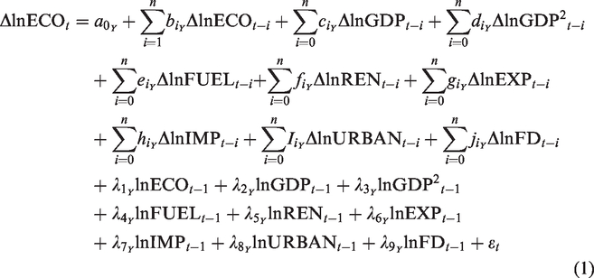
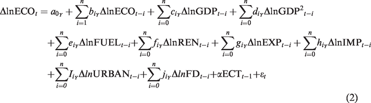
After revealing the long-run equilibrium relationship among variables in Equation 1, short-run and long-run coefficients were estimated by adopting the ECM. The speed of adjustment of the short-run values of the regressors to the long-run equilibrium level of the dependent variable was also estimated by the following ECM model:

\begin{array}{l} Δ \ln EC O_{t} = a_{0_{Y}} + \sum_{i = 1}^{n} b_{i_{Y}} Δ \ln EC O_{t - i} + \sum_{i = 0}^{n} c_{i_{Y}} Δ \ln GD P_{t - i} + \sum_{i = 0}^{n} d_{i_{Y}} Δ \ln GD P^{2} t - i \\ + \sum_{i = 0}^{n} e_{i_{Y}} Δ \ln FUE L_{t - i} + \sum_{i = 0}^{n} f_{i_{Y}} Δ \ln RE N_{t - i} + \sum_{i = 0}^{n} g_{i_{Y}} Δ \ln EX P_{t - i} + \sum_{i = 0}^{n} h_{i_{Y}} Δ \ln IM P_{t - i} \\ + \sum_{i=0}^{n} I_{i_{Y}} {Δln URBAN}_{t - i} + \sum_{i=0}^{n} j_{i_{Y}} {Δln FD}_{t - i} +α {ECT}_{t - 1} {+ε}_{t} \end{array}

(2)

where

{ECT}_{t - 1}

represents the speed of adjustment to the long-run equilibrium level. Goodness of fit of the ARDL model should be investigated by several diagnostic tests. In this study, presence of serial correlation, functional form, normality, and heteroscedasticity were tested by diagnostic tests. Also, the stability of the ARDL model was tested by Brown, Durbin, and Evans¹¹² using cumulative sum (CUSUM) and cumulative sum of squares (CUSUMSQ) in the long run, as well as in the short run, as suggested by Pesaran and Pesaran.¹¹³

Causality test

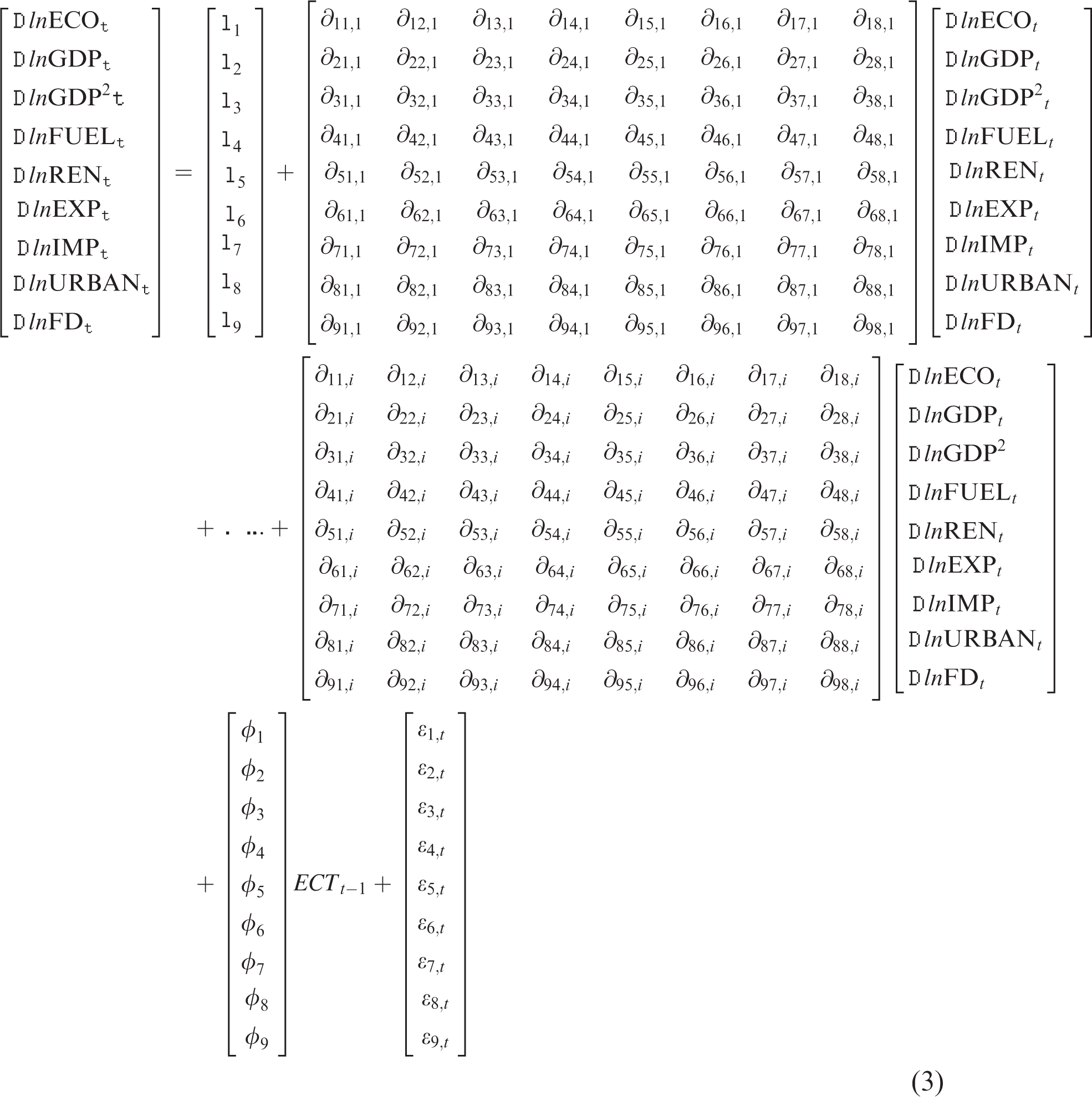
This study employs the Granger causality test through the ECM in order to estimate the directions of possible long-run equilibrium relationships among the variables.

The Granger causality test suggested the estimation of the following ECM:

\begin{array}{l} [\begin{array}{l} {Δln ECO}_{t} \\ {Δln GDP}_{t} \\ {Δln GDP}^{2} t \\ {Δln FUEL}_{t} \\ {Δln REN}_{t} \\ \begin{array}{l} Δln {EXP}_{t} \\ Δln {IMP}_{t} \end{array} \\ {Δln URBAN}_{t} \\ {Δln FD}_{t} \end{array}] = [\begin{array}{l} μ_{1} \\ μ_{2} \\ μ_{3} \\ μ_{4} \\ \begin{array}{l} μ_{5} \\ μ_{6} \end{array} \\ μ_{7} \\ μ_{8} \\ μ_{9} \end{array}] + [\begin{array}{l} \partial_{11, 1} & \partial_{12, 1} & \partial_{13, 1} & \partial_{14, 1} & \partial_{15, 1} & \partial_{16, 1} & \partial_{17, 1} & \partial_{18, 1} \\ \partial_{21, 1} & \partial_{22, 1} & \partial_{23, 1} & \partial_{24, 1} & \partial_{25, 1} & \partial_{26, 1} & \partial_{27, 1} & \partial_{28, 1} \\ \partial_{31, 1} & \partial_{32, 1} & \partial_{33, 1} & \partial_{34, 1} & \partial_{35, 1} & \partial_{36, 1} & \partial_{37, 1} & \partial_{38, 1} \\ \partial_{41, 1} & \partial_{42, 1} & \partial_{43, 1} & \partial_{44, 1} & \partial_{45, 1} & \partial_{46, 1} & \partial_{47, 1} & \partial_{48, 1} \\ \begin{array}{l} \partial_{51, 1} \\ \partial_{61, 1} \end{array} & \begin{array}{l} \partial_{52, 1} \\ \partial_{62, 1} \end{array} & \begin{array}{l} \partial_{53, 1} \\ \partial_{63, 1} \end{array} & \begin{array}{l} \partial_{54, 1} \\ \partial_{64, 1} \end{array} & \begin{array}{l} \partial_{55, 1} \\ \partial_{65, 1} \end{array} & \begin{array}{l} \partial_{56, 1} \\ \partial_{66, 1} \end{array} & \begin{array}{l} \partial_{57, 1} \\ \partial_{67, 1} \end{array} & \begin{array}{l} \partial_{58, 1} \\ \partial_{68, 1} \end{array} \\ \partial_{71, 1} & \partial_{72, 1} & \partial_{73, 1} & \partial_{74, 1} & \partial_{75, 1} & \partial_{76, 1} & \partial_{77, 1} & \partial_{78, 1} \\ \partial_{81, 1} & \partial_{82, 1} & \partial_{83, 1} & \partial_{84, 1} & \partial_{85, 1} & \partial_{86, 1} & \partial_{87, 1} & \partial_{88, 1} \\ \partial_{91, 1} & \partial_{92, 1} & \partial_{93, 1} & \partial_{94, 1} & \partial_{95, 1} & \partial_{96, 1} & \partial_{97, 1} & \partial_{98, 1} \end{array}] [\begin{array}{l} {Δln ECO}_{t} \\ {Δln GDP}_{t} \\ {Δln GDP}^{2} t \\ {Δln FUEL}_{t} \\ \begin{array}{l} Δln {REN}_{t} \\ Δln {EXP}_{t} \end{array} \\ {Δln IMP}_{t} \\ {Δln URBAN}_{t} \\ {Δln FD}_{t} \end{array}] \\ + \dots . . + [\begin{array}{l} \partial_{11, i} & \partial_{12, i} & \partial_{13, i} & \partial_{14, i} & \partial_{15, i} & \partial_{16, i} & \partial_{17, i} & \partial_{18, i} \\ \partial_{21, i} & \partial_{22, i} & \partial_{23, i} & \partial_{24, i} & \partial_{25, i} & \partial_{26, i} & \partial_{27, i} & \partial_{28, i} \\ \partial_{31, i} & \partial_{32, i} & \partial_{33, i} & \partial_{34, i} & \partial_{35, i} & \partial_{36, i} & \partial_{37, i} & \partial_{38, i} \\ \partial_{41, i} & \partial_{42, i} & \partial_{43, i} & \partial_{44, i} & \partial_{45, i} & \partial_{46, i} & \partial_{47, i} & \partial_{48, i} \\ \partial_{51, i} & \partial_{52, i} & \partial_{53, i} & \partial_{54, i} & \partial_{55, i} & \partial_{56, i} & \partial_{57, i} & \partial_{58, i} \\ \begin{array}{l} \partial_{61, i} \\ \partial_{71, i} \end{array} & \begin{array}{l} \partial_{62, i} \\ \partial_{72, i} \end{array} & \begin{array}{l} \partial_{63, i} \\ \partial_{73, i} \end{array} & \begin{array}{l} \partial_{64, i} \\ \partial_{74, i} \end{array} & \begin{array}{l} \partial_{65, i} \\ \partial_{75, i} \end{array} & \begin{array}{l} \partial_{66, i} \\ \partial_{76, i} \end{array} & \begin{array}{l} \partial_{67, i} \\ \partial_{77, i} \end{array} & \begin{array}{l} \partial_{68, i} \\ \partial_{78, i} \end{array} \\ \partial_{81, i} & \partial_{82, i} & \partial_{83, i} & \partial_{84, i} & \partial_{85, i} & \partial_{86, i} & \partial_{87, i} & \partial_{88, i} \\ \partial_{91, i} & \partial_{92, i} & \partial_{93, i} & \partial_{94, i} & \partial_{95, i} & \partial_{96, i} & \partial_{97, i} & \partial_{98, i} \end{array}] [\begin{array}{l} {Δln ECO}_{t} \\ {Δln GDP}_{t} \\ {Δln GDP}^{2} \\ {Δln FUEL}_{t} \\ {Δln REN}_{t} \\ \begin{array}{l} Δln {EXP}_{t} \\ Δln {IMP}_{t} \end{array} \\ {Δln URBAN}_{t} \\ {Δln FD}_{t} \end{array}] \\ + [\begin{array}{l} ϕ_{1} \\ ϕ_{2} \\ ϕ_{3} \\ ϕ_{4} \\ ϕ_{5} \\ ϕ_{6} \\ ϕ_{7} \\ \begin{array}{l} ϕ_{8} \\ ϕ_{9} \end{array} \end{array}] {ECT}_{t - 1} + [\begin{array}{l} ε_{1,t} \\ ε_{2,t} \\ ε_{3,t} \\ ε_{4,t} \\ ε_{5,t} \\ ε_{6,t} \\ ε_{7,t} \\ \begin{array}{l} ε_{8,t} \\ ε_{9,t} \end{array} \end{array}] \end{array}

(3)

where Δ indicates the difference of the variables. The ECT_t−1 is the lagged error correction term, which was estimated from the long-run equilibrium model. Finally, ε_1,t, ε_2,t, ε_3,t, ε_4,t, ε_5,t, ε_6,t, ε_7,t, ε_8,t, and ε_9,t are serially independent random errors with a mean of zero and a finite covariance matrix. According to the Granger causality test through the ECM, statistically significant t-ratios for ECT_t−1 suggest the existence of long-run causal relationships, while statistically significant F-ratios suggest short-run causal relationships among variables.¹¹⁴

Empirical results

ADF and PP tests were applied in order to investigate the integration orders of the variables in the conducted models.^a All variables for Turkey and Mexico were not stationary at their level forms, and they became stationary when their first differences were taken, meaning that they were all integrated of the same order, I(1). On the other hand, fuel energy consumption and trade openness for the case of Indonesia and financial development and fuel energy consumption for Nigeria were stationary at their level forms, meaning that they were integrated of order zero. In summary, ADF and PP unit root test results provided a mixed order of integration of the variables for Indonesia and Nigeria, while variables for Turkey and Mexico had the same order of integration.

The level of relationships among environmental degradation, real income, squared real income, fuel energy consumption, renewable energy consumption, exports, imports, urbanization, and financial development were revealed by the bounds test under the ARDL approach for MINT countries individually. Table 1 indicates the results of the bounds test for the level of relationship. F-statistics for scenarios 3 and 5 of Pesaran et al.¹¹⁰ were compared with the critical values of Narayan¹¹¹ for small samples, and t-statistics were compared with the critical values of Pesaran et al.¹¹⁰ in order to reject the null hypothesis of there being no level relationships among variables.

Table 1.

Bounds test results for level relationship.

	With deterministic trend		Without deterministic trend
Countries	F_V	t_V	F_III	t_III	Conclusion
Mexico
					H₀ rejected
p = 1*	13.051^a	−6.197^a	13.532^a	−6.308^a
2	4.908^a	−3.370^a	4.781^a	−3.692^a
3	3.163^a	−2.028^a	2.841^a	−2.854^a
4	3.276^a	−2.515^a	3.528^a	−3.247^a
Indonesia
					H₀ rejected
p = 3*	4.125^a	−2.682^a	4.160^b	−2.722^c
4	3.313^a	−1.852^a	3.665^b	−2.158^c
5	2.849^a	−1.302^c	3.043^b	−1.553^b
6	3.042^a	−2.139^a	3.051^b	−2.242^b
Nigeria
					H₀ rejected
p = 1*	7.656^c	−4.509^c	2.686^a	−2.476^c
2	5.526^b	−3.733^b	1.752^c	−1.816^c
3	3.801^b	−2.387^b	0.765^b	−0.061^b
4	3.405^b	−2.194^b	0.836^b	0.326^b
Turkey
					H₀ rejected
p = 1*	12.370^c	−5.864^c	8.915^a	−5.121^c
2	6.296^b	−4.302^b	6.104^c	−4.232^c
3	2.002^b	−2.108^b	1.886^b	−2.255^b
4	1.196^b	−0.572^b	1.433^b	−0.662^b

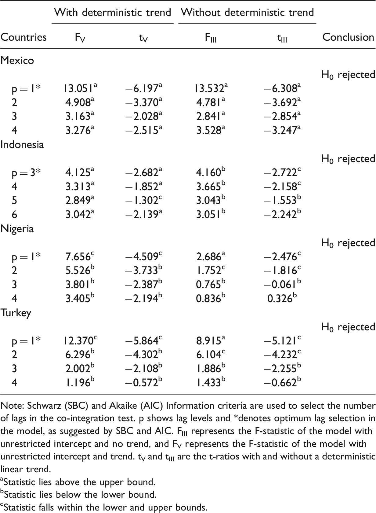
Note: Schwarz (SBC) and Akaike (AIC) Information criteria are used to select the number of lags in the co-integration test. p shows lag levels and *denotes optimum lag selection in the model, as suggested by SBC and AIC. F_III represents the F-statistic of the model with unrestricted intercept and no trend, and F_V represents the F-statistic of the model with unrestricted intercept and trend. t_V and t_III are the t-ratios with and without a deterministic linear trend.

Statistic lies above the upper bound.

Statistic lies below the lower bound.

Statistic falls within the lower and upper bounds.

After revealing the level relationship between variables in the conducted models, the robustness of the ARDL models was investigated. Existence of serial correlation, functional form, normality, and heteroscedasticity were investigated by calculating Lagrange multiplier (LM) and F-statistics for the ARDL models. Diagnostic test results in Table 2 suggest that the ARDL models for the MINT countries have no diagnostic problems as probability values of both LM and F-statistics are insignificant at a 5% level of alpha.

Table 2.

Diagnostic test results.

Test statistics	LM version	F version
Mexico
Serial correlation	0.206 (.650)	0.106 (.748)
Functional form	0.517 (.472)	0.268 (.610)
Normality	4.450 (.108)	–
Heteroscedasticity	0.255 (.613)	0.244 (.624)
Indonesia
Serial correlation	0.257 (.612)	0.155 (.697)
Functional form	0.371 (.542)	0.225 (.639)
Normality	3.368 (.186)	–
Heteroscedasticity	0.149 (.699)	0.142 (.708)
Nigeria
Serial correlation	0.369 (.543)	0.232 (.634)
Functional form	2.763 (.096)	1.855 (.185)
Normality	1.921 (.383)	–
Heteroscedasticity	0.010 (.919)	0.009 (.922)
Turkey
Serial correlation	1.665 (.197)	1.197 (.283)
Functional form	2.582 (.108)	1.899 (.179)
Normality	2.535 (.282)	–
Heteroscedasticity	0.406 (.524)	0.390 (.536)

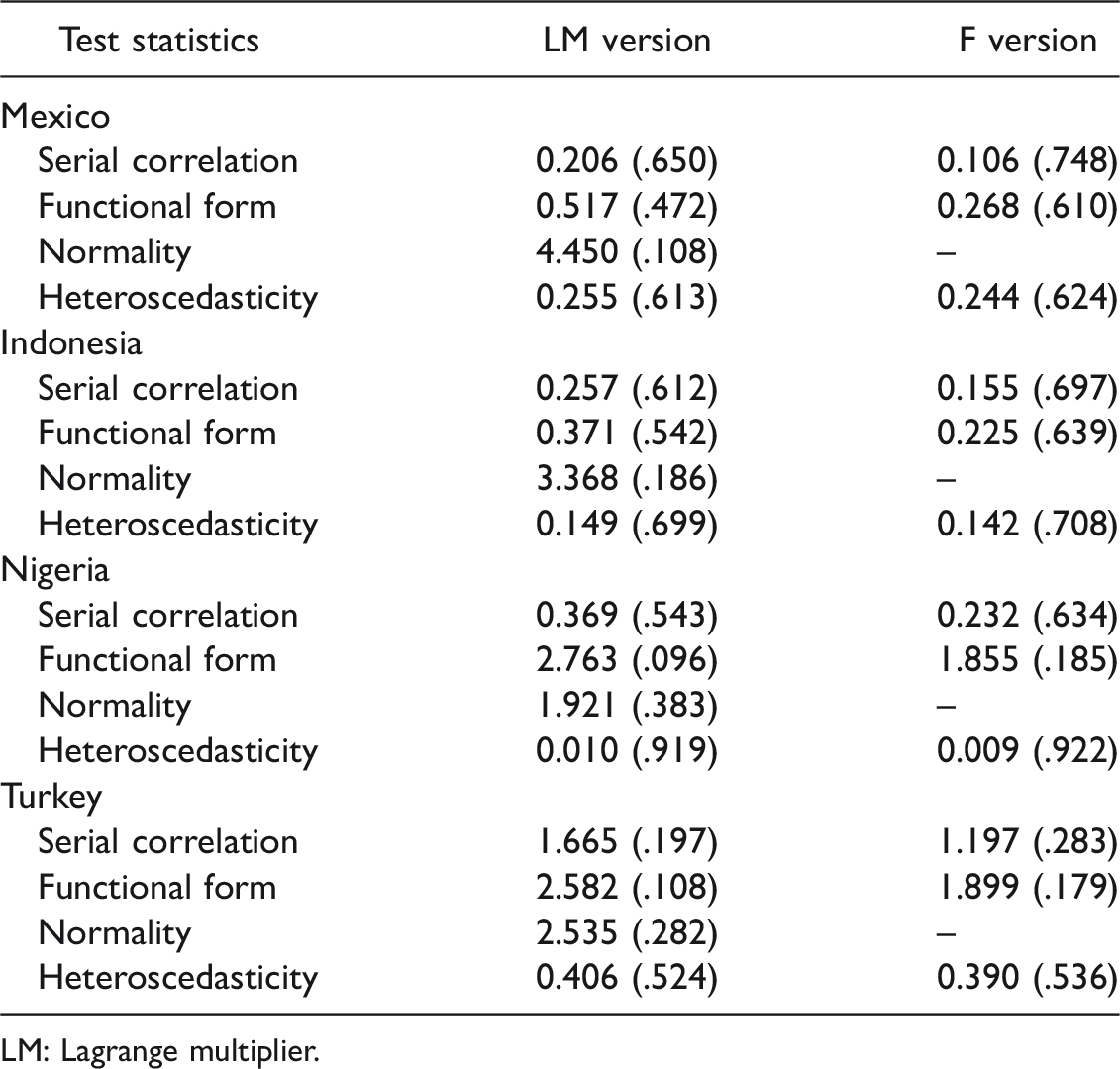
LM: Lagrange multiplier.

The stability of the ARDL models was investigated using the CUSUM and CUSUMSQ methods. Figure 1 indicates the CUSUM and CUSUMSQ graphs for Mexico, Indonesia, Nigeria, and Turkey, respectively. According to these methods, the conducted ARDL models were stable in both the long and the short run.

Figure 1.

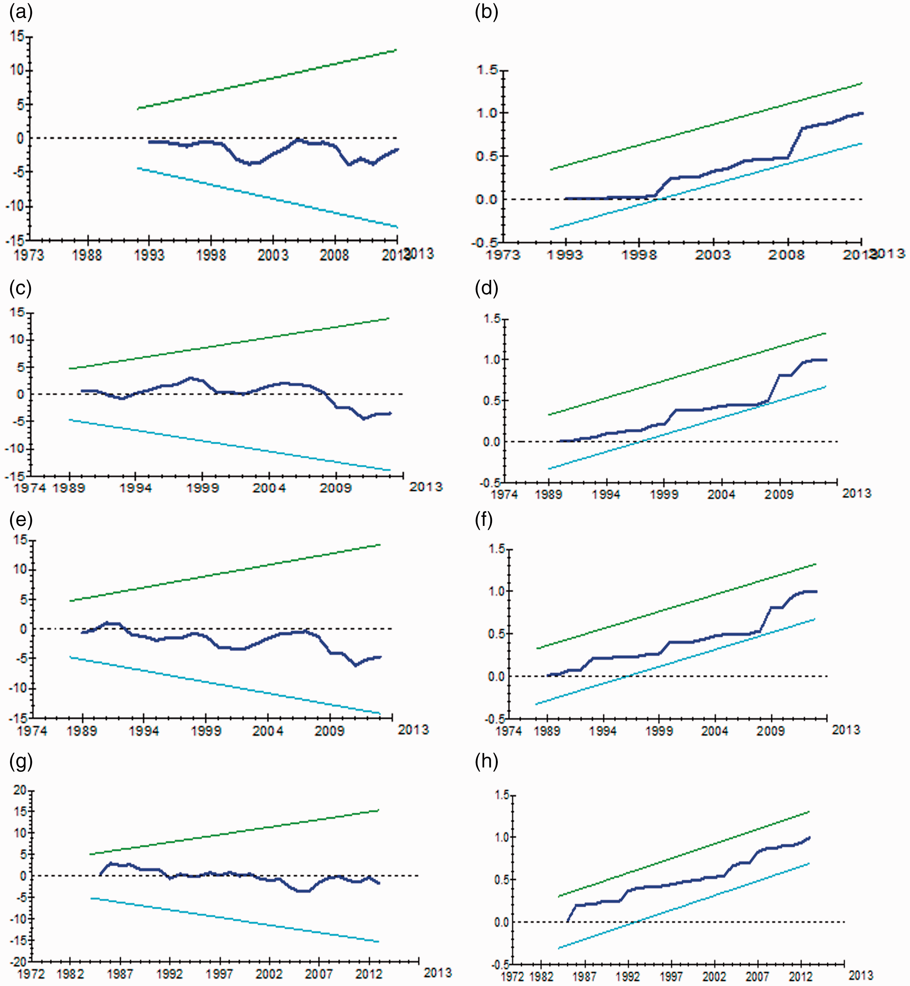
Stability test results. (a) CUSUM for Mexico, (b) CUSUMSQ for Mexico, (c) CUSUM for Indonesia, (d) CUSUMSQ for Indonesia, (e) CUSUM for Nigeria, (f) CUSUMSQ for Nigeria, (g) CUSUM for Turkey, and (h) CUSUMSQ for Turkey. The straight lines represent critical bounds at 5% significance level. CUSUM: cumulative sum; CUSUMSQ: cumulative sum of squares.

The level coefficients were estimated by applying separate long-run ARDL models for each country individually. Table 3 summarizes the results of the long-run ARDL estimations. The existence of the EKC hypothesis can be tested by comparing the long-run coefficients of the GDP and squared GDP. If the coefficient of the GDP is statistically significant and positive while the squared GDP is statistically significant and negative, the EKC hypothesis holds for the host country. When we compared the estimated long-run coefficients of the GDP and the squared GDP for Mexico, Indonesia, Nigeria, and Turkey, respectively, the estimated coefficients of the GDP were statistically significant and positive while the estimated coefficients of the squared GDPs were negative. Our findings suggest the existence of the EKC hypothesis for the cases of MINT countries. Turning points of per capita GDPs for Mexico, Indonesia, Nigeria, and Turkey are calculated as US$14,013, US$4483, US$2079, and US$14,705, respectively. These findings indicate that turning points of Mexico, Indonesia, and Turkey are not within the range of sample per capita GDP, meaning that they have not reached their turning points yet. On the other hand, turning point of Nigeria is within the sample per capita GDP. Our empirical findings show that in term of implied turning point there is no uniformity among the countries under investigation.

Table 3.

Level coefficients in the long-run model through the autoregressive distributed lag approach.

Dependent variable		Regressors
	lnGDP	lnGDP²	lnFUEL	lnREN	lnEXP	lnIMP	lnURBAN	lnFD	Intercept	Trend
Mexico
lnECO	28.185**	−1.476**	3.883**	−0.054	0.362*	−0.129	1.013*	−0.294*	−75.742*	–
	(0.031)	(0.041)	(0.024)	(0.777)	(0.000)	(0.121)	(0.000)	(0.001)	(0.001)	–
Indonesia
lnECO	3.481**	−0.207**	0.314**	0.377**	−0.293*	0.250*	0.591*	−0.094*	0.471	−0.067
	(0.022)	(0.032)	(0.032)	(0.031)	(0.006)	(0.006)	(0.002)	(0.000)	(0.934)	(0.521)
Nigeria
lnECO	3.830***	−0.250***	0.426**	−3.477*	−0.062**	0.175*	−1.313*	−0.050*	5.627	–
	(0.074)	(0.083)	(0.000)	(0.000)	(0.031)	(0.000)	(0.000)	(0.000)	(0.589)	–
Turkey
lnECO	12.763*	−0.665*	4.279*	−0.442**	−0.106*	0.072**	0.825*	−0.009	−25.508*	0.035*
	(0.000)	(0.000)	(0.000)	(0.011)	(0.000)	(0.033)	(0.001)	(0.793)	(0.009)	(0.006)

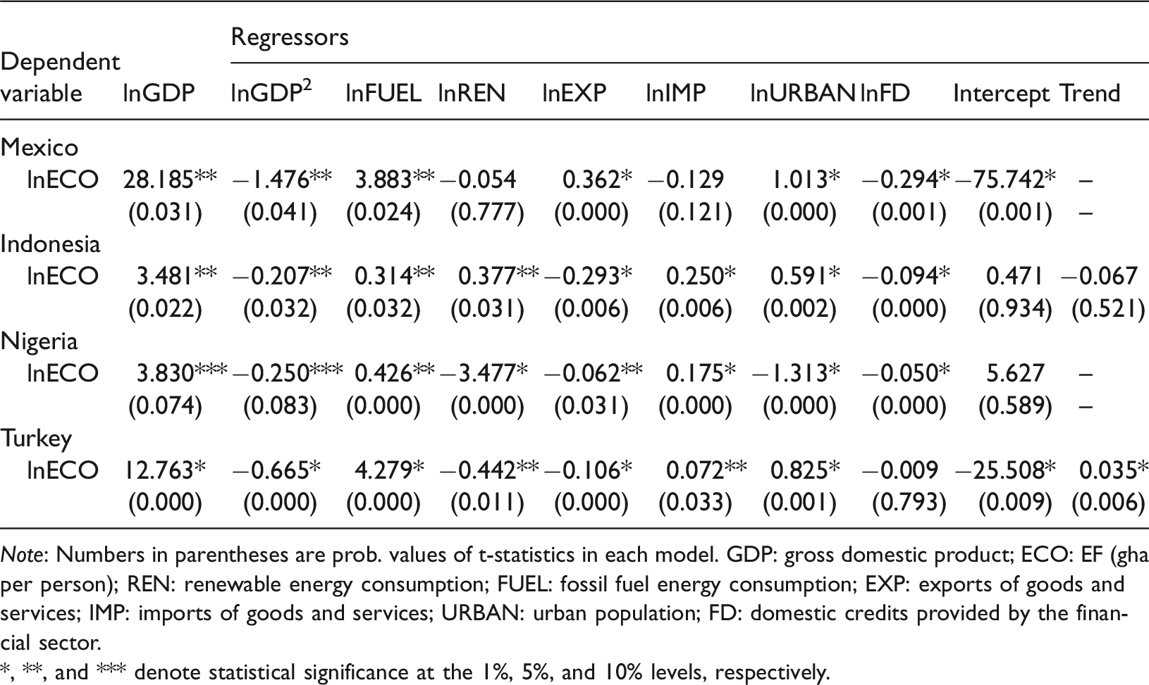
Note: Numbers in parentheses are prob. values of t-statistics in each model. GDP: gross domestic product; ECO: EF (gha per person); REN: renewable energy consumption; FUEL: fossil fuel energy consumption; EXP: exports of goods and services; IMP: imports of goods and services; URBAN: urban population; FD: domestic credits provided by the financial sector.

*, **, and *** denote statistical significance at the 1%, 5%, and 10% levels, respectively.

The findings of the ARDL estimations suggest that, in the long run, fossil fuel energy consumption, exports, urbanization, and financial development are the common significant determinants of the EF, which is used as a proxy for environmental degradation for the cases of the MINT countries. Renewable energy consumption is statistically significant and has an elastic, negative impact on the EF for the cases of Mexico, Nigeria, and Turkey. This finding suggests that increasing the usage of renewable energy reduces the environmental degradation, and this contradicts the findings of Apergis et al.¹¹⁵ and Bölük and Mert.⁸⁷ In the literature, exports and imports are well-known determinants of environmental degradation. Our findings indicate that imports contribute to environmental degradation in Indonesia, Nigeria, and Turkey, while exports reduce the environmental degradation, meaning that imports increase the domestic consumption and contribute to EF of the host countries. Our results are consistent with Liddle⁹⁵ and Hasanov, Liddle, and Mikayilov.¹¹⁶ Moreover, urbanization in Indonesia, Turkey, and Mexico have a statistically significant and positive impact on the EF in the long run. On the other hand, there is a significant long-run negative relationship between urbanization and EF in Nigeria. The estimated negative impact of urbanization in the case of Mexico supports the findings of Ozturk et al.⁸⁰ Finally, financial development has statistically significant and negative impact on EF for the case of Mexico, Indonesia, and Nigeria, meaning that these countries are successful in allocating their financial resources to improve environmental quality in the long run.

The speed of adjustments and short-run coefficients were estimated by adopting the ECM through the ARDL approach. Table 4 indicates the results of the ECMs through the ARDL approach for the cases of MINT countries. The ECM models suggest that the EFs of the MINT countries converge to their long-run equilibrium levels by 162.4%, 93.7%, 68.4%, and 99.9% speed of adjustments every year by the contributions of the short-run values of the GDP, GDP squared, fuel, renewable energy consumption, exports, imports, urbanization, and financial development, respectively. In addition, there are statistically significant short-run impacts of regressors on the EF at different lag levels for the cases of the MINT countries.

Table 4.

Conditional error correction model through the autoregressive distributed lag approach.

Dependent variable	MexicolnECO(1,0,2,2,2,2,0,1,2)*		IndonesialnECO(0,2,2,0,0,1,0,0,0)*		NigerialnECO(2,0,0,2,0,0,1,2,2)*		TurkeylnECO(1,1,2,0,0,0,0,1,0)*
Regressor	Coefficient	p	Coefficient	p	Coefficient	p	Coefficient	p
û_t−1	−1.624	0.000	−0.937	0.000	−0.684	0.000	−0.999	0.000
ΔlnECO(−1)	–	–	–	–	−0.322	0.001	–	–
ΔlnGDP	10.328	0.637	4.157	0.190	−1.772	0.438	9.957	0.012
ΔlnGDP(−1)	–	–	9.299	0.005	–	–	–	–
ΔlnGDP²	−0.567	0.642	−0.244	0.237	0.129	0.406	−0.488	0.026
ΔlnGDP²(−1)	−0.145	0.000	−0.641	0.003	–	–	−0.013	0.029
ΔlnFUEL	5.673	0.005	−0.227	0.043	0.337	0.001	1.763	0.016
ΔlnFUEL(−1)	11.906	0.000	−	−	0.142	0.005	−	−
ΔlnREN	0.944	0.002	0.263	0.006	−2.031	0.003	−0.314	0.057
ΔlnREN(−1)	1.833	0.000	−	−	−	−	−	−
ΔlnIMP	−0.164	0.017	0.181	0.000	0.097	0.000	0.111	0.000
ΔlnEXP	0.381	0.000	−0.129	0.000	−0.055	0.000	−0.109	0.000
ΔlnEXP(−1)	−0.374	0.000	−	−	−	−	−	−
ΔlnURBAN	−47.617	0.000	0.998	0.033	5.339	0.000	0.744	0.143
ΔlnURBAN(−1)	104.038	0.000	−	−	−4.811	0.000	−	−
ΔlnFD	−0.303	0.000	−0.086	0.000	−0.094	0.000	−0.068	0.183
ΔlnFD(−1)	−	−	−	−	0.011	0.183	−	−
Intercept	−0.047	0.183	−0.011	0.345	−0.001	0.920	0.001	0.888
R²		0.902		0.788		0.787		0.923
Standard error of regression		0.037		0.014		0.022		0.024
F-prob.		0.000		0.000		0.000		0.000

Note: GDP: gross domestic product; ECO: EF (gha per person); REN: renewable energy consumption; FUEL: fossil fuel energy consumption; EXP: exports of goods and services; IMP: imports of goods and services; URBAN: urban population; FD: domestic credits provided by the financial sector.

*p-lag structures in the model.

The directions of the long-run relationships among variables were revealed by adopting Granger causality test through the vector error correction model. Results of the Granger causality test are summarized in Appendix 1. Panels (a), (b), (c), and (d) indicate results of the causality test for the cases of Mexico, Indonesia, Nigeria, and Turkey, respectively. There are unidirectional causal relationships running from the GDP, squared GDP, renewable energy consumption, fuel energy consumption, exports, imports, urbanization, and financial development to the EF. Unidirectional causal relationships suggest that, when there is a change in real income, squared real income, renewable energy and fossil fuel energy consumption, exports, imports, urbanization, and financial development, respectively, there is a change in the EF of MINT countries. Moreover, as it can be seen in panel (b), there are unidirectional causal relationships running from the GDP, squared GDP, renewable energy consumption, fuel energy consumption, exports, imports, financial development, and the EF to urbanization for the case of Indonesia. Causal relationships which are running from energy consumption variables to urbanization are in line with Liddle and Lung.¹¹⁷

Conclusion

Our study investigated the validity of the EKC hypothesis for each of the MINT countries. In contrast to the majority of empirical studies that use a single variable as a measure for the environmental pollution to test the EKC hypothesis, we used a more inclusive measure, namely, the EF as a proxy for the pressure on the environment. We used a time series approach to estimate the country-based coefficients which enabled us to identify the most suitable policy implications for each country in our sample. The long-run equilibrium relationships among the EF, fossil fuel energy, renewable energy consumption, exports, imports, financial development, and urbanization were revealed by adopting the bounds testing approach for the cases of the MINT countries. The ARDL model estimations confirmed the validity of the EKC hypothesis for each of the four countries under investigation. Another common finding for each of these countries is the significant effects of exports, urbanization, and fossil fuel consumption on the environmental degradation index. This finding signifies the importance of energy efficiency in emerging countries. In order to increase their energy efficiency, emerging countries should take some actions to achieve the usage of clean energy in their industries. Creating financial incentives, such as tax credits, subsidies, and grants, and setting national regulations can lead to increases in the adoption of clean technology and, in turn, efficient usage of energy by polluting industries. They can also provide an award mechanism to encourage polluting industries to adopt clean energy.

Our results show that the effects of renewable energy, international trade, urbanization, and financial development differ among these countries. Financial development has statistically significant and negative impacts for Mexico, Indonesia, and Nigeria, which means that financial systems of the host countries are successful to direct the financial resources to environmental friendly sectors. Financial resources can be used to increase the level of public awareness and to encourage polluting industries to adopt clean energy and new pollution mitigating technologies by providing subsidies and soft loans. Also, financial resources can be used to encourage polluting industries for investing in environmental friendly projects to reduce environmental degradation. The inverse relationship between urbanization and environmental pressure that was observed in Nigeria shows that the urban planning strategies of these countries can overcome the negative effects of urbanization on the use of environment. The long-run coefficient of renewable energy consumption for the cases of Nigeria and Turkey suggests a negative relationship between renewable energy and environmental pollution. This finding indicates that increasing the level of renewable energy consumption for these countries is a possible solution for environmental pollution. The policy makers of Mexico and Indonesia should invest more in research and development (R&D) activities in order to achieve the efficient usage of renewable energy and promote the adoption of clean technology in the production phase of renewable energy. Another remarkable result, in terms of policy implementation, is the effects of exports and imports on environmental pollution. Exports contribute to the environmental quality in Indonesia, Nigeria, and Turkey, while imports increase the level of environmental degradation. Policy makers of these three countries should be aware of the positive impacts of imports and take precautions against the negative impact of imports on environmental quality.

Footnotes

Declaration of conflicting interests

The authors declared no potential conflicts of interest with respect to the research, authorship, and/or publication of this article.

Funding

The authors received no financial support for the research, authorship, and/or publication of this article.

Note

Eyup Dogan is an Associate Professor of Economics in the School of Management and Leadership at Abdullah Gül University (AGÜ), Turkey. He received his PhD in Economics from Clemson University, USA, in 2014. His teaching and research interests lie on macroeconomics, energy and environmental economics and applied econometrics. He has currently over 30 papers in peer-reviewed journals such as Renewable Energy, RSER, Energy, ESPR, Energy Sources Part B, Sustainable Cities and Society (>800 citations and H-index: 14). He is serving as member of Editorial Board and reviewer of numerous journals.

Nigar Taspinar is an Assistant Professor of Finance in the Department of Banking and Finance at Eastern Mediterranean University (EMU), North Cyprus. She received her PhD in Finance from Eastern Mediterranean University, North Cyprus, in 2016. Her teaching and research interests lie on Financial Management, Energy and Environmental Economics, Energy Finance, Applied Financial Statistics and Applied Econometrics. She has published several research papers in international peer-reviewed journals. Amongst these include Renewable and Sustainable Energy Reviews, Science of the Total Environment, Energy & Environment, The Service Industries Journal, International Trade and Economic Development and Environmental Science and Pollution Research.

Korhan K Gokmenoglu graduated from Middle East Technical University, Brandeis University, Essec University and worked as visiting scholar at University of California San Diego. Currently, he is an Associate Professor at the Department of Banking and Finance in the Eastern Mediterranean University. His research field focuses on applied econometrics, energy economics, environmental degradation, and macroeconomics. His research studies have been published in many international peer-reviewed journals, including Computation and Economic Cybernetics Studies and Research, Croatian Operational Research Review, Economic Systems, Energy, Energy & Environment, Environmental Science and Pollution Research, Science of the Total Environment, Singapore Economic Review, The Journal of International Trade & Economic Development, and International Trade & Economic Development. Also, he has served as a referee for many prestigious academic journals.

Appendix 1

References

Grossman

Krueger

AB.

Environmental impacts of a North American free trade agreement. NBER working paper no. 3914. Cambridge: National Bureau of Economic Research, 1991.

Selden

Song

Environmental quality and development: is there a Kuznets curve for air pollution emissions?

J Environ Econ Manage 1994; 27: 147–162.

Bimonte

Stabile

Land consumption and income in Italy: a case of inverted EKC. Ecol Econ 2017; 131: 36–48.

A literature survey on environmental Kuznets curve. Energy Procedia 2011; 5: 1322–1325.

Dong

Wang

Guo

The global EKCs. Int Rev Econ Financ 2016; 43: 210–221.

Kaika

Zervas

The environmental Kuznets curve (EKC) theory—part A: concept, causes and the CO₂ emissions case. Energy Policy 2013; 62: 1392–1402.

Saboori

Sulaiman

Mohd

Economic growth and CO₂ emissions in Malaysia: a cointegration analysis of the environmental Kuznets curve. Energy Policy 2012; 51: 184–191.

Apergis N and Ozturk I. Testing environmental Kuznets curve hypothesis in Asian countries. Ecological Indicators 2015; 52: 16–22.

Balaguer

Cantavella

Estimating the environmental Kuznets curve for Spain by considering fuel oil price (1874–2011). Ecol Indic 2016; 60: 853–859.

10.

Bilgili F, Koçak E, and Bulut Ü. The dynamic impact of renewable energy consumption on CO2 emissions: a revisited Environmental Kuznets Curve approach. Renewable and Sustainable Energy Reviews 2016; 54: 838–845.

11.

Charfeddine

Mrabet

The impact of economic development and social-political factors on ecological footprint: a panel data analysis for 15 MENA countries. Renew Sustain Energy Rev 2017; 76: 138–154.

12.

Heidari

Katircioğlu

Saeidpour

Economic growth, CO₂ emissions, and energy consumption in the five ASEAN countries. Int J Electr Power Energy Syst 2015; 64: 785–791.

13.

Kasman

Duman

YS.

CO₂ emissions, economic growth, energy consumption, trade and urbanization in new EU member and candidate countries: a panel data analysis. Econ Model 2015; 44: 97–103.

14.

Wang

Zhao

Environmental Kuznets curve in China: new evidence from dynamic panel analysis. Energy Policy 2016; 91: 138–147.

15.

Mrabet

Alsamara

Testing the Kuznets curve hypothesis for Qatar: a comparison between carbon dioxide and ecological footprint. Renew Sustain Energy Rev 2017; 70: 1366–1375.

16.

Pablo-Romero

Cruz

Barata

Testing the transport energy-environmental Kuznets curve hypothesis in the EU27 countries. Energy Econ 2017; 62: 257–269.

17.

Wang Y, Han R and Kubota J. Is there an environmental Kuznets curve for SO2 emissions? A semi-parametric panel data analysis for China. Renewable and Sustainable Energy Reviews 2016; 54: 1182–1188.

18.

Wackernagel

Rees

WE.

(1996). Our ecological footprint: reducing human impact on the earth. Gabriola Island: New Society Publishers.

19.

Al-Mulali

Saboori

Ozturk

Investigating the environmental Kuznets curve hypothesis in Vietnam. Energy Policy 2015; 76: 123–131.

20.

Dietz

Rosa

York

Driving the human ecological footprint. Front Ecol Environ 2007; 5: 13–18.

21.

Jorgenson

AK.

Consumption and environmental degradation: a cross-national analysis of the ecological footprint. Soc Probl 2003; 50: 374–394.

22.

Jorgenson AK. Uneven processes and environmental degradation in the world-economy. Human Ecology Review 2004; 11(2): 103–117.

23.

Jorgenson

Burns

TJ.

The political-economic causes of change in the ecological footprints of nations, 1991–2001. Soc Sci Res 2007; 36: 834–853.

24.

Jorgenson

Rice

Structural dynamics of international trade and material consumption: a cross-national study of the ecological footprints of less developed countries. J World Syst Res 2005; 11: 57–77.

25.

Rothman

DS.

Environmental Kuznets curves—real progress or passing the buck?

Ecol Econ 1998; 25: 177–194.

26.

York

Rosa

Dietz

Footprints on the earth: the environmental consequences of modernity. Am Soc Rev 2003; 68: 279–300.

27.

York

Rosa

Dietz

The ecological footprint intensity of national economies. J Ind Ecol 2004; 8: 139–154.

28.

York

Rosa

Dietz

A tale of contrasting trends: three measures of the ecological footprint in China, India, Japan, and the United States, 1961-2003. J World Syst Res 2009; 15: 134–146.

29.

Vackar

Ecological footprint, environmental performance and biodiversity: a cross-national comparison. Ecol Indic 2012; 16: 40–46.

30.

Adeolu

The MINT countries as emerging economic power bloc: prospects and challenges. Dev Ctry Stud 2013; 4: 99–106.

31.

Boesler

The economist who invented the BRICs just invented a whole new group of countries: the MINTs. Bus Insider 2013; 13. https://www.businessinsider.com.au/jim-oneill-presents-the-mint-economies-2013-11

32.

Fraser

Fidelity is confident its MINTs won’t suck. London: Bloomsbury Information, 2011.

33.

Magalhaes

O‘Neill, man who coined ‘BRICs’, Still likes BRICs, but likes MINTs, too. The Wall Street Journal, 2013. December 9

34.

Wright

After the BRICS are the MINTs, but can you make any money from them? www.forbes.com/sites/chriswright/2014/01/06/after-the-brics-the-mints-catchy-acronym-but-can-you-make-any-money-from-it/#7cd59d0429a6 (2014, accessed 17 February 2019).

35.

Ghosh

Electricity consumption and economic growth in Taiwan. Energy Policy 2002; 30: 125–129.

36.

Jumbe

CBL.

Co-integration and causality between electricity consumption and GDP: empirical evidence from Malawi. Energy Econ 2004; 26: 61–68.

37.

Mehrara

Energy consumption and economic growth: the case of oil exporting countries. Energy Policy 2007; 35: 2939–2945.

38.

Nnaji

Unachukwu

Uzoma

CC.

Electricity generation, economic growth and the need for alternative source of power in Nigeria. Niger J Sol Energy 2011; 22: 177–182.

39.

Nnaji

Chukwu

Uzoma

CC.

(2013). An econometric study of CO2 emissions, energy consumption, foreign trade and economic growth in Nigeria. In: Conference proceedings of the 5th annual NAEE/IAEE international conference organized by Nigerian Association for Energy Economics, Abuja, Nigeria, 23–24 April 2012, pp. 489–508. Nigerian Association for Energy Economics.

40.

Shiu

Lam

PL.

Electricity consumption and economic growth in China. Energy Policy 2004; 32: 47–54.

41.

ECOWAS Renewable Energy. Baseline report for the ECOWAS renewable energy policy (EREP). Final draft, 23 October 2012. ECOWAS Centre for Renewable Energy and Energy Efficiency.

42.

Kraft

On the relationship between energy and GNP. J Energy Dev 1978; 3: 401–403.

43.

Tibaa

Omri

Literature survey on the relationships between energy, environment and economic growth. Renew Sustain Energy Rev 2017; 69: 1129–1146.

44.

Dasgupta

Mody

Roy

, et al. Environmental regulation and development: a cross-country empirical analysis. Oxford Dev Stud 2001; 29: 173–187.

45.

Kuznets

Economic growth and income inequality. Am Econ Rev 1955; 45: 1–28.

46.

Shafik

Economic development and environmental quality: an econometric analysis. Oxford Econ Pap 1994; 46: 757–773.

47.

Shafik

Bandyopadhyay

Economic growth and environmental quality: time series and cross-section evidence. Background paper for the world development report. Washington, DC: The World Bank, 1992.

48.

Özokcu

Özdemir

Ö.

Economic growth, energy, and environmental Kuznets curve. Renew Sustain Energy Rev 2017; 72: 639–647.

49.

Katz

Water use and economic growth: reconsidering the environmental Kuznets curve relationship. J Clean Prod 2015; 88: 205–213.

50.

Lin

Omoju

Nwakeze

, et al. Is the environmental Kuznets curve hypothesis a sound basis for environmental policy in Africa? J Clean Prod 2016; 133: 712–724.

51.

Ahmad

, et al. Modelling the CO₂ emissions and economic growth in Croatia: is there any environmental Kuznets curve? Energy 2017; 123: 164–172.

52.

Jaunky

VC.

The CO₂ emissions-income nexus: evidence from rich countries. Energy Policy 2011; 39: 1228–1240.

53.

Chow

Environmental Kuznets curve: conclusive econometric evidence for CO₂. Pac Econ Rev 2014; 19: 1–7.

54.

Alvarez-Herranz

Balsalobre-Lorente

Shahbaz

, et al. Energy innovation and renewable energy consumption in the correction of air pollution levels. Energy Policy 2017; 105: 386–397.

55.

Anatasia V. The Causal Relationship between GDP,Exports, Energy Consumption, and CO2 in Thailand andMalaysia. International Journal of Economic Perspectives 2015; 9(4): 37–48.

56.

Lorente

Álvarez-Herranz

Economic growth and energy regulation in the environmental Kuznets curve. Environ Sci Pollut Res 2016; 23: 16478–16494.

57.

Shahbaz

Lean

Shabbir

MS.

Environmental Kuznets curve hypothesis in Pakistan: cointegration and Granger causality. Ren Sustain Energy Rev 2012; 16: 2947–2953.

58.

Cetin

Ecevit

The impact of financial development on carbon emissions under the structural breaks: empirical evidence from Turkish economy. Int J Econ Perspect 2017; 11: 64–78.

59.

De Bruyn

Van den Bergh

JCJM

Opschoor

JB.

Economic growth and emissions: reconsidering the empirical basis of environmental Kuznets curves. Ecol Econ 1998; 25: 161–175.

60.

Zambrano-Monserrate

Fernandez

MA.

An environmental Kuznets curve for N₂O emissions in Germany: an ARDL approach. Nat Resour Forum 2017; 41: 119–127.

61.

Harbaugh

Levinson

Wilson

DM.

Reexamining the empirical evidence for an environmental Kuznets curve. Rev Econ Stat 2002; 84: 541–551.

62.

Liddle

Messinis

Revisiting sulfur Kuznets curves with endogenous breaks modeling: substantial evidence of inverted-Us/Vs for individual OECD countries. Econ Model 2015; 49: 278–285.

63.

Llorca

Meunié

SO₂ emissions and the environmental Kuznets curve: the case of Chinese provinces. J Chin Econ Business Stud 2009; 7: 1–16.

64.

Xiaoyu

Jun

Pengfei

Structure and application of a new comprehensive environmental pollution index. Energy Procedia 2011; 5: 1049–1054.

65.

Thompson

Environmental Kuznets curve for water pollution: the case of border countries. Mod Econ 2014; 5: 66–69.

66.

Mills

Waite

TA.

Economic prosperity biodiversity conservation, and the environmental Kuznets curve. Ecol Econ 2009; 68: 2087–2095.

67.

Chowdhury

Moran

Turning the curve: a critical review of Kuznets approaches. Appl Geogr 2012; 32: 3–11.

68.

Almeida

TAN

Cruz

Barata

, et al. Economic growth and environmental impacts: an analysis based on a composite index of environmental damage. Ecol Indic 2017; 76: 119–130.

69.

Stern

DI.

The environmental Kuznets curve: a primer. CCEP working paper no. 1404. 2014. Australian National University, Centre for Climate Economic & Policy.

70.

Ulucak

Lin

Persistence of policy shocks to ecological footprint of the USA. Ecol Indic 2017; 80: 337–343.

71.

García-Sánchez

Almeida

TAN

Camara

RPB.

A proposal for a composite index of environmental performance (CIEP) for countries. Ecol Indic 2015; 48: 171–188.

72.

Teixidó-Figueras

Duro

JA.

The building blocks of international ecological footprint inequality: a regression-based decomposition. Ecol Econ 2015; 118: 30–39.

73.

Uddin

Alam

Gow

Does ecological footprint impede economic growth? An empirical analysis based on the environmental Kuznets curve hypothesis. Aust Econ Pap 2016; 55: 301–316.

74.

Uddin

Salahuddin

Alam

, et al. Ecological footprint and real income: panel data evidence from the 27 highest emitting countries. Ecol Indic 2017; 77: 166–175.

75.

Mostafa

MM.

A Bayesian approach to analyzing the ecological footprint of 140 nations. Ecol Indic 2010; 10: 808–817.

76.

Acar

Aşıcı

AA.

Nature and economic growth in Turkey: what does ecological footprint imply?

Middle East Dev J 2017; 9: 101–115.

77.

Al-Mulali

Weng-Wai

Sheau-Ting

, et al. Investigating the environmental Kuznets curve (EKC) hypothesis by utilizing the ecological footprint as an indicator of environmental degradation. Ecol Indic 2015; 48: 315–323.

78.

Bagliani

Bravo

Dalmazzone

A consumption-based approach to environmental Kuznets curve using the ecological indicator. Ecol Econ 2008; 65: 650–661.

79.

Boutaud

Natacha

Christian

Local environmental quality versus (global) ecological carrying capacity: what might alternative aggregated indicators bring to the debates about environmental Kuznets curves and sustainable development?

Int J Sustain Dev 2006; 9: 297–310.

80.

Ozturk

Al-Mulali

Saboori

Investigating the environmental Kuznets curve hypothesis: the role of tourism and ecological footprint. Environ Sci Pollut Res 2016; 23: 1916–1928.

81.

Saboori

Al-Mulali

Baba

, et al. Oil-induced environmental Kuznets curve in organization of petroleum exporting countries (OPEC). Int J Green Energy 2016; 13: 408–416.

82.

Wang

Kang

, et al. Estimating the environmental Kuznets curve for ecological footprint at the global level: a spatial econometric approach. Ecol Indic 2013; 34: 15–21.

83.

Caviglia-Harris

Chambers

Kahn

JR.

Taking the U out of Kuznets: a comprehensive analysis of the EKC and environmental degradation. Ecol Econ 2009; 68: 1149–1159.

84.

Al-Mulali

Tang

Ozturk

Does financial development reduce environmental degradation? Evidence from a panel study of 129 countries. Environ Sci Pollut Res 2015; 22: 14891–14900.

85.

Asıcı

Acar

Does income growth relocate ecological footprint?

Ecol Indic 2016; 61: 707–714.

86.

Khan

SAR

Zaman

Zhang

The relationship between energy-resource depletion, climate change, health resources and the environmental Kuznets curve: evidence from the panel of selected developed countries. Renew Sustain Energy Rev 2016; 62: 468–477.

87.

Bölük

Mert

Fossil & renewable energy consumption, GHGs (greenhouse gases) and economic growth: evidence from a panel of EU (European Union) countries.

Energy 2014; 74: 439–446.

88.

Omri A. An international literature survey on energy-economic growth nexus: Evidence from country-specific studies. Renewable and Sustainable Energy Reviews 2014; 38, 951–959.

89.

Bölük

Mert

The renewable energy, growth and environmental Kuznets curve in Turkey: an ARDL approach. Renew Sustain Energy Rev 2015; 52: 587–595.

90.

Balsalobre-Lorente

Shahbaz

Energy consumption and trade openness in the correction of GHG levels in Spain. Bull Energy Econ 2016; 4: 310–322.

91.

Lopez

Islam

AM.

Trade and the environment. Princet Encyclop World Econ 2007; 16: 35–51.

92.

Taylor

MS.

Unbundling the pollution haven hypothesis. Adv Econ Anal Policy 2005; 3: 29.

93.

Ali W, Abdullah Aand Azam M. Re-visiting the environmental Kuznets curve hypothesis for Malaysia: fresh evidence from ARDL bounds testing approach. Renewable and sustainable energy reviews 2017; 77: 990–1000.

94.

Andersson

Lindroth

Ecologically unsustainable trade. Ecol Econ 2001; 37: 113–122.

95.

Liddle

Consumption-based accounting and the trade-carbon emissions nexus. Energy Econ 2018; 69: 71–78.

96.

Jalil

Feridun

The impact of growth, energy and financial development on the environment in China: a cointegration analysis. Energy Econ 2011; 33: 284–291.

97.

Katircioglu

Taspinar

Testing the moderating role of financial development in an environmental Kuznets curve: empirical evidence from Turkey. Renew Sustain Energy Rev 2017; 68: 572–586.

98.

Tamazian

Bhaskara Rao

Do economic, financial and institutional developments matter for environmental degradation? Evidence from transitional economies. Energy Econ 2010; 32: 137–145.

99.

Begum

Sohag

Abdullah

SMS

, et al. CO₂ emissions, energy consumption, economic and population growth in Malaysia. Renew Sustain Energy Rev 2015; 41: 594–601.

100.

Dogan

Turkekul

CO₂ emissions, real output, energy consumption, trade, urbanization and financial development: testing the EKC hypothesis for the USA. Environ Sci Pollut Res 2015; 23: 1–11.

101.

Hossain

Panel estimation for CO₂ emissions, energy consumption, economic growth, trade openness and urbanization of newly industrialized countries. Energy Policy 2011; 39: 6991–6999.

102.

Katircioglu

Kilinc

CC.

Investigating the role of urban development in the conventional environmental Kuznets curve: evidence from the globe. Environ Sci Pollut Res Int 2018; 25: 15029–15035.

103.

Ozturk

Al-Mulali

Investigating the validity of the environmental Kuznets curve hypothesis in Cambodia. Ecol Indic 2015; 57: 324–330.

104.

Shahbaz

Sbia

Hamdi

, et al. Economic growth, electricity consumption, urbanization and environmental degradation relationship in United Arab Emirates. Ecol Indic 2014; 45: 622–631.

105.

World Bank Development. World development indicators, http://databank.worldbank.org (2017, accessed 17 February 2019).

106.

Global Footprint Network Database. Global Footprint Network. http://data.footprintnetwork.org/#/ (2017, accessed 17 February 2019).

107.

OECD Database. OECD statistics. https://data.oecd.org/ (2017, accessed 17 February 2019).

108.

Dickey

Fuller

WA.

Likelihood ratio statistics for autoregressive time series with a unit root. Econometrica 1981; 49: 1057–1072.

109.

Phillips

Perron

Testing for a unit root in time series regression. Biometrica 1988; 75: 335–346.

110.

Pesaran

Shin

Smith

RJ.

Bounds testing approaches to the analysis of level relationships. J Appl Econ 2001; 16: 289–326.

111.

Narayan

PK.

The saving and investment nexus for China: evidence from cointegration tests. Appl Econ 2005; 37: 1979–1990.

112.

Brown

Durbin

Evans

JM.

Techniques for testing the constancy of regression relations over time. J R Stat Soc 1975; 37: 149–163.

113.

Pesaran

Working with Microfit 4.0: interactive econometric analysis. Oxford: Oxford University Press, 1997.

114.

Narayan

Smyth

Crime rates, male youth unemployment and real income in Australia: evidence from Granger causality tests. Appl Econ 2004; 36: 2079–2095.

115.

Apergis

Payne

Menyah

, et al. On the causal dynamics between emissions, nuclear energy, renewable energy, and economic growth. Ecol Econ 2010; 69: 2255–2260.

116.

Hasanov

Liddle

Mikayilov

JI.

The impact of international trade on CO₂ emissions in oil exporting countries: territory vs consumption emissions accounting. Energy Econ 2018; 74: 343–350.

117.

Liddle

Lung

Might electricity consumption cause urbanization instead? Evidence from heterogeneous panel long-run causality tests. Glob Environ Change 2014; 24: 42–51.

118.

BBC. The Mint countries: next economic giants? www.bbc.com/news/magazine-25548060 (2014, accessed 24 September 2017).