Measuring technical inefficiency and CO 2 shadow price of Korean fossil-fuel generation companies using deterministic and stochastic approaches

Abstract

This paper measures the technical inefficiency and the shadow price of Korean fossil-fuel generation companies (GENCOs) between 2001 and 2016 at the firm-level. To obtain robust empirical results, this study employs both commonly used deterministic and stochastic estimation methods. The empirical results are as follows: the inefficiency estimates are approximately 0.09 (deterministic) and 0.08 (stochastic); the estimates of CO₂ shadow price, in KRW/tCO₂, are 82,758 (deterministic) and 49,830 (stochastic), which shows high volatility in the annual average shadow price. In addition, we find that the results of the deterministic method without any random errors show a large variation in the trends of technical inefficiency and shadow price, while the stochastic method with random errors yields only moderate volatility. Our empirical results are expected to assist policymakers in determining how much potential mitigation can be achieved through improved efficiency, and the range of the CO₂ shadow price will contribute to more efficient policy tools.

Keywords

Fossil-fuel generation companies shadow price technical inefficiency directional distance function

Introduction

Fossil-fuel power plants generated 57–68% of the total electricity produced in Korea during 2001–2015, of which coal-fired electricity generation accounted for 58–71%.¹ Burning fossil fuels produces byproducts such as $N O_{x}$ , $S O_{x}$ and ${CO}_{2}$ which are harmful to the environment and human beings.² Among these harmful pollutants, ${CO}_{2}$ emissions are considered a primary cause of climate change. Various international cooperative attempts have been made to mitigate ${CO}_{2}$ emissions, such as the Kyoto Protocol and the Paris Agreement.

Korea is one of the most intensive ${CO}_{2}$ emitters in the OECD. The average annual growth rate of ${CO}_{2}$ emissions in Korea during 1991–2000 was 6.15%, which was the second-highest among the OECD member countries. For the period of 2001–2014, ${CO}_{2}$ emissions growth was 2.06%, which was the third-highest among OECD member nations.³ In spite of this dramatic decline in the ${CO}_{2}$ emission growth rate, the comparison with other OECD countries implies that Korea needs to further reduce ${CO}_{2}$ emissions.^a The Korean government set the goal of reducing greenhouse gas (GHG) emissions by 37% below business-as-usual (BAU) levels by 2030 and established the Roadmap to Achieve the National GHG Reduction Target in December 2016.⁴ Under the Framework Act on Low Carbon, Green Growth in 2010, the emissions trading scheme (K-ETS) was launched in 2015, and subsequently, an auction system for GHG emissions allowances was established in 2019 to achieve GHG emission reduction targets.⁵ The operation of the K-ETS is based on the Coase theorem that bargaining leads to the efficient allocation of outcomes regardless of the initial assignment of property rights.⁶

As of 2015, the ${CO}_{2}$ emissions of five fossil-fuel generation companies (GENCOs) accounted for 28.5% of the total ${CO}_{2}$ emissions in Korea. These GENCOs include Namdong Power (59.1 mil. ${CO}_{2}$ ), Dongseo Power (40.0 mil. ${CO}_{2}$ ), Seobu Power (33.8 mil. ${CO}_{2}$ ), Jungbu Power (33.7 mil. ${CO}_{2}$ ), and Nambu Power (32.1 mil. ${CO}_{2}$ ), ranked second to sixth in total ${CO}_{2}$ emissions in Korea, respectively.^b

During 2001–2016, Korea’s annual average growth rate of electric consumption was 4.06%, which was significantly higher than the OECD’s average growth rate of 0.73%.⁷ This rapid growth in Korea’s electric consumption is mainly the result of low electricity rates. Many organizations and households convert their energy sources to electric power to take advantage of low electricity rates, and the share of electricity of total energy consumed in Korea increased from 17.5% in 2007 to 19.3% in 2012. The capital-intensive structure of Korean industry also drives the increase in electricity consumption. This trend demands that the Korean economy manages electricity production efficiently through mitigating ${CO}_{2}$ emissions in electricity production.

The main objective of this study is to measure the technical (in)efficiency and estimate the marginal abatement cost (MAC), or shadow price, of ${CO}_{2}$ for GENCOs in Korea at the firm-level.^c It extends existing empirical research by capturing firm specific bureaucratic and administrative characteristics of GENCOs related to technical (in)efficiency and MAC of ${CO}_{2}$ . It also enables us to compare the relationship of GENCOs’ operational performance and ${CO}_{2}$ emissions and determine appropriate strategies for each firm to deal with ${CO}_{2}$ emissions. We employed both deterministic and stochastic methods to obtain robust empirical results. Firm-level data for inputs and outputs of GENCOs between 2001 and 2016 was used in the empirical investigation.

The estimation of the MAC of ${CO}_{2}$ is one of the primary research topics in energy and environmental studies since it enables the approximation of the ${CO}_{2}$ emission allowance price in emission trading markets.^2,9 Various methods have been employed in estimating the MAC because the true value of the MAC is difficult to obtain. Although the concept of shadow price is one way of estimating the MAC from engineering and economic perspectives,¹⁰ this study focuses on the economic perspective of shadow price.

The literature estimated the technical inefficiency and the MAC of ${CO}_{2}$ , but they showed inconsistent results. Their large variations in technical efficiency and ${CO}_{2}$ MAC are largely due to their different data sets, units of analysis, and time of analysis. Types of empirical methodologies also lead to inconsistent results.¹¹

We utilized deterministic and stochastic approaches commonly employed in estimating the MAC as a determinant of shadow price because the literature concluded that there is no single method superior to others. Thus, there is a need to examine the shadow price of ${CO}_{2}$ emissions with distinctive methods.¹¹ We show that the average technical inefficiency ranges from 0.083 to 0.085 and ${CO}_{2}$ MAC ranges from 29,722–128,444 $KRW / t {CO}_{2}$ using the deterministic approach, and ranges from 34,644–64,135 $KRW / t {CO}_{2}$ using the stochastic approach. The technical inefficiency and shadow prices show different patterns across methodologies to varying extents.

Our study have examined firm-level inefficiency and shadow prices to offer insights on climate change policy. The previous studies focused on the plant-level analysis,^5,10,12 leading to insufficient policy implications for each firm. Our approach has advantage in designing new government policy incentives tailored to each GENCO. Also, from the firm perspective, our results provide GENCOs with their explicit shadow price that enables GENCOs with low CO2 shadow price to seek new business opportunities.

The remainder of this paper is as follows. Literature review section discusses the methodological exposition used in this study. Methodology section describes the data set for the empirical investigation. Data section shows the empirical results, and Empirical results section briefly concludes this study.

Literature review

Scholars have widely examined technical (in)efficiency associated with environmental issues. They measure technical (in)efficiency to evaluate the current progress toward established targets and suggest policy and strategic recommendations.^d For example, Lu and Lu¹⁴ investigated that energy efficiency was 0.7426 for 28 countries, based on fossil fuel ${CO}_{2}$ emissions at the country level in the European Union. Choi et al.¹⁵ estimated the energy efficiency, potential emission reductions, and MAC in different provinces of China. Ji and Zhou¹⁶ found the inefficiency estimate for 105 Chinese cities was 0.03, incurring the MACs of ${CO}_{2}$ , ${SO}_{2}$ and ${NO}_{x}$ emissions. Lee and Zhang¹⁷ measured the technical efficiencies and shadow prices for 30 Chinese manufacturing industries to identify potential reductions of ${CO}_{2}$ emissions.

Previous studies have also focused on technical (in)efficiency in South Korea. Lee¹⁸ investigated the Korean electric power plants with a focus on fuel inputs and found that the plants could save 22% per year in fuel costs based on allocative efficiency analysis. In contrast to studies introduced earlier, Choi and Oh¹⁹ examined new product efficiency at the product level in the vehicle market. These examples showed that environmental studies use efficiency analysis in diverse topics and feature various units of analysis.

Previous studies have also examined the efficiency of the power generation sector. The concept of the directional distance function (DDF) is usually used in estimating technical (in)efficiency and the MAC because the power sector generates electricity and produces byproducts simultaneously. Kwon and Yun²⁰ estimated the MAC of the Korean power generation sector during 1990–1995 using parametric DDF and found that the average technical efficiency was 0.93. Murty et al.,²¹ on the other hand, applied the directional output distance function with a stochastic frontier to estimate the technical and environmental inefficiency of the coal-fired thermal power generation facilities and found it ranged from 0.023 to 0.100 in India. Rezek and Campbell²² demonstrated the use of the maximum entropy approach in a distance function framework and estimated the efficiency of 260 US electric plants in 1998 as 0.78. Lee⁵ estimated the shadow price of ${CO}_{2}$ for 52 power generators in the Korean electric generation industry in 2007 using output distance function and found that the efficiency is 0.98.

Some studies estimated the MAC of ${CO}_{2}$ depending on their research goals. Kwon and Yun²⁰ estimated the average ${CO}_{2}$ MAC as 3,800 KRW/ $tC O_{2}$ between 1990 and 1995 in the Korean power generation sector. Park and Lim¹² found that the shadow price of ${CO}_{2}$ is 14.04 EUR/ $tC O_{2}$ during 2001–2004 for Korean fossil fuel power plants. In India, the average ${CO}_{2}$ MAC was found to be approximately 2402–3381 INR/ $tC O_{2}$ between 1991 and 2000 (Gupta, 2006). Rezek and Campbell²² priced ${CO}_{2}$ MAC for US plants in 1998 at 18.10 USD/ $tC O_{2}$ . In China, the shadow prices of ${CO}_{2}$ were found to be 7.2, 44.1, and 61.1–105.0 USD/ $tC O_{2}$ at the level of province, city, and industry, respectively.^11,15,16 The ${CO}_{2}$ MAC in Japan was found to be 38.9 USD/ $tC O_{2}$ during 2000–2009.⁸

Table 1 summarizes the estimated efficiencies and shadow prices of ${CO}_{2}$ from previous studies and most used a parametric methodology.^e In this summary, we can recognize the large variations in technical efficiency and ${CO}_{2}$ MAC across previous studies. These inconsistent results are due to the different data sets used, units of analysis, time of analysis, and empirical methodologies. Most prior studies chose one empirical methodology only, but we test the technical (in)efficiency and ${CO}_{2}$ MAC with both deterministic and stochastic approaches at the firm-level and then interpret findings with a focus on the Korean context and firm-level analysis.

Table 1.

Comparison between CO₂ shadow prices of present and previous studies.

Study	Data (observations, unit, country, time)	Estimation Method	Efficiency	Shadow Price of CO₂ (USD per ton)
Kwon and Yun²⁰	57, plant, Korea, 1990–1995	Deterministic Trans-log ODF	0.93	$4.9
Gupta²³	76, plant, India, 1991–2000	Deterministic Trans-log ODF	0.97	$77.5, $55.1
Murty et al.²¹	480, plant, India, 1997–2004	Stochastic Quadratic DDF	0.90–0.98
Rezek and Campbell²²	260, plant, United States, 1998	Stochastic Maximum Entropy ODF	0.78	$18.1
Park and Lim¹²	80, plant, Korea, 2001–04	Deterministic Trans-log ODF		$18.1
Lee⁵	52, generator, Korea, 2007	Deterministic Trans-log ODF	0.98	$14.6
Matsushita and Yamane⁸	76, company, Japan, 2000–2009	Deterministic Quadratic DDF	0.97	$38.9
Lee et al.¹⁰	111, plant, Korea, 2004–2008	Non-parametric DEA	0.84–0.86	$21.6–40.5
Zhou et al.¹¹	30, industry, China, 2009–2011	Deterministic ODF, IDF & DDF		$61.1–105.0
Ji and Zhou¹⁶	907, city, China, 2006–2014	Deterministic Quadratic DDF	0.97	$44.1
This Study	80, firm, Korea, 2001–2016	Deterministic (LP) & Stochastic (COLS) DDF	0.92	$70.6 (LP), $42.5 (COLS)

Note: 1. The currency of Kwon and Yun²⁰ is converted using the exchange rate in 1995; Gupta²³ with the one in 99–00; Park and Lim,¹² Zhou et al.,¹¹ and Ji and Zhou¹⁶ are with 2005’s, 2011’s, and 2006’s, respectively; and for this study, we used the rate in 2015.

2. ODF: output distance function, DDF: directional distance function, IDF: input distance function.

3. In some cases, efficiency is calculated with the inefficiency estimate.

Methodology

This section discusses our use of the directional distance function (DDF) to estimate the inefficiency and shadow price of Korean fossil-fuel GENCOs. Underlying assumptions section provides the underlying assumptions, and then Directional distance function, inefficiency and shadow price section and Estimation of shadow price section discuss the parametric approach used to measure inefficiency and shadow price.

Underlying assumptions

Production technology is represented by the production possibility set (PPS), as follows:

Ψ (x) = {(y, b) | x canproduce (y, b)}

(1)

where

x

is an input vector,

x \in R_{+}^{N}

;

y

is a desirable output vector,

y \in R_{+}^{M}

; and

b

is an undesirable output vector,

b \in R_{+}^{J}

. We assume that there are

K

decision-making units (DMUs; in this study, Korean fossil-fuel GENCOs).

We posit the following axioms on the PPS.:

The PPS is compact for each input vector, x \in R_{+}^{N}

(2)

(0, 0) \in Ψ (x) for all x \in R_{+}^{N}

(3)

if x^{'} \geq x then P (x^{'}) \supseteq Ψ (x)

(4)

if (y, b) \in P (x) and b = 0, then y = 0

(5)

if (y, b) \in P (x) and 0 \leq θ \leq 1 then (θ y, θ b) \in P (x)

(6)

if (y, b) \in Ψ (x) and y^{'} \leq y, then (y^{'}, b) \in Ψ (x)

(7)

The axiom in equation (2) means that a finite amount of inputs produces a finite amount of outputs. The axiom in equation (3) represents that inactivity is always possible. The axiom in equation (4) posits the strong disposability of inputs, meaning that the PPS will not shrink if inputs are increased (or not reduced). The null-jointness axiom is posited in equation (5), indicating that it is not possible to produce desirable outputs without the production of undesirable outputs. The weak disposability of desirable and undesirable outputs is imposed in equation (6), indicating that any contraction in the original production of desirable and undesirable outputs are always possible if the original combination of desirable and undesirable outputs is producible. Equation (7) reflects the strong disposability of desirable outputs, meaning that any output vector with less desirable outputs is always possible if the original combination of desirable and undesirable output is producible. An in-depth discussion on the above six axioms can be found in Färe et al.²⁴

Directional distance function, inefficiency and shadow price

The representation of production discussed in Underlying assumptions section is valuable from the theoretical perspective. However, it is not helpful in calculating the shadow price of undesirable outputs and the inefficiencies of DMUs. For this step, the directional distance function (DDF) is commonly used.^f The DDF is defined as follows:

D (x, y, b; g_{y}, - g_{b}) = {β | (y + β g_{y}, b - β g_{b}) \in Ψ (x)}

(8)

where the direction vector,

(g_{y}, - g_{b})

, is predetermined by a researcher before estimating the DDF. The DDF simultaneously seeks the amount of a maximum increase in desirable outputs and a maximum decrease in undesirable outputs, which is interpreted as (in)efficiency. The DDF has the following properties corresponding to those of the PPS.

D (x, y, b; g_{y}, - g_{b}) \geq 0 if and only if (y, b) \in Ψ (x)

(9)

D (x, y^{'}, b; g_{y}, - g_{b}) \geq D (x, y, b; g_{y}, - g_{b}) for (y^{'}, b) \leq (y, b) \in Ψ (x)

(10)

D (x, y, b^{'}; g_{y}, - g_{b}) \geq D (x, y, b; g_{y}, - g_{b}) for (y, b^{'}) \geq (y, b) \in Ψ (x)

(11)

D (x, θ y, θ b; g_{y}, - g_{b}) \geq 0 for (y, b) \in Ψ (x) and 0 \leq θ \leq 1

(12)

D (x, y + α g_{y}, b - α g_{b}; g_{y}, - g_{b}) = D (x, y, b; g_{y}, - g_{b}) - α, α \in R

(13)

D (x, y, b; g_{y}, - g_{b}) is concave in (y, b) \in Ψ (x)

(14)

The above properties can be translated into positivity (9), monotonicity in desirable output (10), monotonicity in undesirable output (11), weak disposability of outputs (12), translation (13), and concavity (14). These properties are well described in Färe et al.²⁴ The translation property shown in equation (13) is important. If desirable outputs are expanded by the amount, $α g_{y}$ and undesirable outputs are contracted by the amount, $α g_{b}$ , the inefficiency is reduced by $α$ . Hence, the DDF with the direction vector of $(g_{y}, - g_{b}) = (1, - 1)$ provides us with the actual amount of increase in desirable outputs and the actual amount of decrease in undesirable outputs until the original inefficiency is removed.²⁴ The sum of DDFs with the same direction vector provides the total increase in desirable outputs and the total decrease in undesirable outputs of DMUs under investigation. The average DDF in any sample is equivalent to the expected increase in desirable outputs, and the expected decrease in undesirable outputs of a typical DMU.

The shadow price is regarded as the unit market value of an unmarketable output corresponding to the decrease in revenue associated with the unit increase in output.^g From the operational research perspective, the shadow price is equivalent to the optimized dual variable of the primal linear programming problem. Therefore, data envelopment analysis (DEA) is widely used in estimating the shadow price of undesirable outputs since DEA employs a linear programming technique in general.¹⁰ However, there are two concerns when using DEA to estimate shadow prices. First, DEA is vulnerable to outliers or extreme observations.²⁵ Since the gradient of an outermost PPS (i.e., frontier) is related to the shadow price, the existence of outliers is likely to yield a distorted estimation of the shadow price. Second, DEA is likely to yield a negative shadow price of undesirable outputs in contrast to the common understanding that undesirable output reduces revenue.¹⁰

Therefore, we use the more general linear programming technique developed by Aigner and Chu.²⁶ The DDF is parameterized with a quadratic function, in which the direction vector $(g_{y}, - g_{b})$ is $(1, - 1)$ . In the empirical analysis, we assume that one desirable output, $y$ , and one undesirable output, $b$ , are produced using two input factors, $x$ . Then, the DDF is formulated as follows:

D (x, y, b; 1, - 1) = α_{0} + \sum_{n = 1}^{2} α_{n} x_{n} + β_{1} y + γ_{1} b + 1 / 2 \sum_{n = 1}^{2} \sum_{n^{'} = 1}^{2} α_{n, n^{'}} x_{n} x_{n^{'}} + 1 / 2 β_{2} y^{2} + 1 / 2 γ_{2} b^{2} + \sum_{n = 1}^{2} ν_{n} x_{n} b + μ y b + \sum_{n = 1}^{2} δ_{n} x_{n} y

(15)

The following constraints are needed for the DDF to satisfy the properties introduced in equations (9)–(14):

D (x, y, b; 1, - 1) \geq 0

(16)

\partial D (x, y, b; 1, - 1) / \partial y = β_{1} + β_{2} y + μ u + \sum_{n = 1}^{2} δ_{n} x_{n} \leq 0

(17)

\partial D (x, y, b; 1, - 1) / \partial u = γ_{1} + γ_{2} u + \sum_{n = 1}^{2} ν_{n} x_{n} + μ y \geq 0

(18)

β_{1} - γ_{1} = - 1, β_{2} = γ_{2} = μ, δ_{n} - ν_{n} = 0, n = 1, 2,

(19)

The positivity is formulated into equation (16), which is true if and only if a DMU is within its PPS.²⁷ Monotonicity of desirable outputs is shown in equation (17), monotonicity in undesirable outputs is shown in equation (18), and the translation is shown in equation (19). The condition of $β_{2} \leq 0$ is the necessary and sufficient condition for concavity. In addition to these constraints, the symmetry condition is needed as follows:

α_{n, n^{'}} = α_{n^{'}, n}, n, n^{'} = 1, 2. 6 f

(20)

In order to obtain parameter estimates, we solve the following linear programming problem, as used in Aigner and Chu.²⁶

In comparison, we also estimate the DDF shown in equation (15) using a stochastic model. We discuss more deeply this stochastic estimation in Empirical results section.

\begin{array}{l} m i n \sum_{k = 1}^{K} (D (x_{k}, y_{k}, {\overset{⌢}{b}}_{k}; 1, - 1) - 0) \\ s . t . D (x_{k}, y_{k}, {\overset{⌢}{b}}_{k}; 1, - 1) \geq 0 for k = 1, \dots, K, \\ \partial D (x_{k}, y_{k}, {\overset{⌢}{b}}_{k}; 1, - 1) / \partial y = {\hat{β}}_{1} + {\hat{β}}_{2} y + \hat{μ} u + \sum_{n = 1}^{2} {\hat{δ}}_{n} x_{n} \leq 0 for k = 1, \dots, K, \\ \partial D (x_{k}, y_{k}, {\overset{⌢}{b}}_{k}; 1, - 1) / \partial b = {\hat{γ}}_{1} + {\hat{γ}}_{2} u + \sum_{n = 1}^{2} {\hat{ν}}_{n} x_{n} + \hat{μ} y \geq 0 for k = 1, \dots, K, \\ {\hat{β}}_{1} - {\hat{γ}}_{1} = - 1, {\hat{β}}_{2} = {\hat{γ}}_{2} = \hat{μ}, {\hat{δ}}_{n} - {\hat{ν}}_{n} = 0, n = 1, 2, \\ {\hat{α}}_{n, n^{′}} = {\hat{α}}_{n^{′}, n} for n, n^{′} = 1, 2 \end{array}

(21)

DMU-specific inefficiency can be calculated from the results of parameter estimates drawn from equation (21) or the stochastic model. We will discuss how to estimate the shadow price in the following subsection.

Estimation of shadow price

When we estimate the shadow price under an economic framework, we need to consider the relationship between PPS and desirable/undesirable outputs. As discussed in Färe et al.,²⁴ many scholars in the 1990s utilized the concept of Shephard’s²⁸ output distance function in which desirable and undesirable outputs are assumed to increase so that a DMU reaches the frontier.^h Previous approaches have limitations in calculating the shadow price of undesirable outputs, and thus, researchers have attempted to develop an advanced methodology, i.e., a directional distance functional approach. The DDF is defined as the minimum distance that makes a DMU reach the frontier of the PPS by following the predetermined direction.ⁱ

We use the asymmetric projection of desirable and undesirable outputs onto the PPS to derive shadow prices of undesirable outputs. As discussed in Directional distance function, inefficiency and shadow price section, we use the direction vector of $(g_{y}, - g_{b}) = (1, - 1)$ . Then, the revenue function of any DMU is as follows:

R (x, y, b) = \max_{y, b} {p y - qb | D (x, y, b; 1, - 1) \geq 0}

(22)

where

p

and

q

are prices of desirable and undesirable outputs, respectively. Note that the positivity property in equation (16) is employed in this revenue function. Based on the Lagrangian method, the shadow price of the

j th

undesirable output is as follows:

q_{j} = - p_{m} [\frac{\partial D (x, y, b; 1, - 1)}{\partial b_{j}} / \frac{\partial D (x, y, b; 1, - 1)}{\partial y_{m}}]

(23)

If the functional form of the directional distance function in equation (15) is used, then the shadow price can be expressed as follows:

q = - p [\frac{γ_{1} + γ_{2} b + μ y + \sum_{n = 1}^{2} ν_{n} x_{n}}{β_{1} + β_{2} y + μ b + \sum_{n = 1}^{2} δ_{n} x_{n}}]

(24)

Note that we have only one desirable output and one undesirable output, for which the subscripts of prices are suppressed in equation (24). The shadow price shown in equation (24) can be interpreted as the value of electricity that must be foregone when all inefficiency is eliminated.²⁴

Data

Our data set consists of five Korean fossil-fuel GENCOs, including Dongseo, Jungbu, Nambu, Namdong, and Seobu, during 2001–2016, which indicates we used a panel data set of 80 observations. The empirical investigation assumes that one desirable output, electric generation (TWh), and one undesirable output, ${CO}_{2}$ emission (mil. ${CO}_{2}$ ), are simultaneously produced. We also assume that two input factors are used in production, i.e., the number of employees (FTE) and capacity (GW). The number of employees is used as a proxy for labor and capacity here is used as a proxy for capital stock. We exclude fuel usage from the empirical analysis because ${CO}_{2}$ emissions and fuel usage are highly correlated.

We collected data for electric generation, the number of employees, and capacity from a power grid company, the Korea Electric Power Corporation (KEPCO), and annual reports of GENCOs. We collected ${CO}_{2}$ emission data from various sources. For the period from 2001–2006, we converted fuel usage into ${CO}_{2}$ emissions as follows: (1) Three types of fuel, i.e., gas, oil, and coal, were converted to a tonne of oil equivalent (TOE). (2) Then, the ${CO}_{2}$ emissions of each fuel type were estimated using carbon conversion factors. (3) Finally, we summed the ${CO}_{2}$ emissions for the three types of fuel. For the period from 2007–2010, we collected ${CO}_{2}$ emissions data from KEPCO. We collected ${CO}_{2}$ emissions from the Greenhouse Gas Inventory and Research Center for the remainder of the study period.

The descriptive statistics of variables are listed in Table 2. The average annual total of ${CO}_{2}$ emissions in Korea is approximately 562 mil. ${CO}_{2}$ during 2001–2016.³¹ Thus, we can infer that the share of ${CO}_{2}$ emissions for each Korean GENCO accounts for around 5.9% of total emissions.^j The average annual electricity generation of each GENCO is 47.60 TWh, and its standard deviation is 10.56. The average annual production capacity and labor are 7.91 GW and 1,817.47 FTE, respectively.

Table 2.

Descriptive statistics (n = 80).

	Mean	Median	Std.dev.	Max	Min
Generation (TWh)	47.60	48.40	10.56	71.51	27.87
CO₂ emissions (mil. CO₂)	33.29	33.30	10.07	59.73	3.38
Capacity (GW)	7.91	8.16	1.29	10.93	4.96
Labor (FTE)	1817.47	1813.50	228.85	2335.00	1342.00

Sources: KEPCO, annual reports of GENCOs and the Greenhouse gas inventory and Research center.

The mean and growth rate of variables for each GENCO are listed in Table 3. The growth rate of electricity generation varies across GENCOs. Namdong showed the highest growth rate in electricity generation (CAGR of 4.9%), and Dongseo showed the lowest growth rate (CAGR of 3.6%). The average ${CO}_{2}$ emissions and the growth rate of ${CO}_{2}$ emissions vary across companies. Namdong showed the highest level of emissions, 40.9 mil. ${CO}_{2}$ , and the highest growth rate of 5.7%. The remaining four GENCOs show a similar ${CO}_{2}$ emissions pattern: 27.7–34.9 mil. ${CO}_{2}$ of mean level and 3.6–4.0% of CAGR.

Table 3.

Descriptive statistics of variables by company (n = 80).

GENCO	Generation (TWh)		CO₂ (mil. CO₂)		Capacity (GW)		Labor (FTE)
GENCO	Mean	CAGR	Mean	CAGR	Mean	CAGR	Mean	CAGR
Dongseo	46.0	3.6	34.9	3.9	8.3	1.7	1927.1	1.4
Jungbu	43.6	4.3	30.9	3.6	7.8	1.5	1987.4	1.2
Nambu	51.1	4.2	32.0	4.0	8.0	3.3	1743.4	1.6
Namdong	51.7	4.9	40.9	5.7	7.6	3.4	1742.9	1.8
Seobu	45.5	3.8	27.7	3.7	7.9	2.0	1686.4	1.3
Average	47.6	4.1	33.3	4.2	7.9	2.3	1817.5	1.5

Note: The CAGR represents the compound annual growth rate, and its unit is %.

Sources: KEPCO, annual reports of GENCOs and the Greenhouse gas inventory and Research center.

The average annual values of input and output variables are listed in Table 4. Electricity generation and ${CO}_{2}$ emissions peaked in 2013. Capacity and labor increased by around 65% and 39%, respectively. The large variation in electricity generation and ${CO}_{2}$ emissions implies that the inefficiency of Korean GENCOs was likely to change to some extent.

Table 4.

Mean of variables over time (n = 80).

Year	Generation (TWh)	CO₂ (mil. CO₂)	Capacity (GW)	Labor (FTE)
2001	31.85	22.60	6.02	1530.00
2002	33.95	23.64	6.17	1512.00
2003	34.72	24.40	6.35	1551.60
2004	38.66	26.61	6.84	1616.20
2005	39.99	27.56	7.05	1695.20
2006	42.12	28.79	7.16	1775.60
2007	46.86	33.15	7.58	1870.20
2008	47.98	34.19	8.23	1882.20
2009	50.92	38.36	8.31	1862.00
2010	56.41	38.69	8.63	1815.00
2011	56.70	41.37	8.54	1806.80
2012	58.52	42.16	8.50	1902.80
2013	60.73	43.06	8.88	2004.60
2014	55.94	40.62	9.16	2042.40
2015	52.54	33.24	9.15	2080.40
2016	53.63	34.15	9.98	2132.60
Average	47.60	33.29	7.91	1817.47

Sources: KEPCO, annual reports of GENCOs and the Greenhouse gas inventory and Research center.

Empirical results

This section provides the estimation results of our model, the technical inefficiency, and the shadow price of ${CO}_{2}$ for Korean GENCOs.

Estimation results

We employed linear programming and stochastic techniques in estimating the parameters of the DDF because there is no superior method in shadow price estimation.¹¹ The DDF shown in equation (6) was estimated using the lpSolve package (ver.5.6.13) and plm package (ver.1.6–6) in R-3.4.3. As discussed in Methodology section, we also used a stochastic model in estimating technical inefficiency and the shadow price of each GENCO over the study period by incorporating random error and inefficiency terms into the models. In doing so, we estimated the quadratic DDF using the stochastic frontier model (SFM) following Kumbhakar and Lovell.³² Our quadratic DDF form is as follows:

0 = D (x, y, b; g_{y}, - g_{b}) + ϵ_{k}

(25)

where

ϵ_{k} = v_{k} - u_{k}

v_{k} \sim N (0, σ_{v}^{2})

and

u_{k} \sim N^{+} (0, σ_{u}^{k}

). The

v_{k}

is an idiosyncratic error term and the

u_{k}

is a technical inefficiency term. In order to estimate equation (25), we need to use the translation property of the DDF with the direction vector of

(g_{y}, - g_{b}) = (1, - 1)

as follows:

D (x_{k}, y_{k} + α_{k} \cdot 1, b - α_{k} \cdot 1; 1, - 1) + α_{k} = D (x_{k}, y_{k}, b_{k}; 1, 1)

(26)

We substitute $D (x_{k}, y_{k}, b_{k}; 1, 1)$ with $D (x_{k}, y_{k} + α_{k} \cdot 1, b - α_{k} \cdot 1; 1, - 1) + α_{k}$ in equation (25). After moving $α_{k}$ to the left-hand side, we obtain:

- α_{k} = D (x_{k}, y_{k} + α_{k} \cdot 1, b_{k} - α_{k} \cdot 1; 1, - 1) + ϵ_{k}

(27)

where

D (x_{k}, y_{k} + α_{k} \cdot 1, b_{k} - α_{k} \cdot 1; 1, - 1)

is the quadratic form shown in equation (15), in which we substitute

y

with

y + α_{k} \cdot 1

and

b

with

b - α_{k} \cdot 1

. An appropriate choice of

α_{k}

is a precondition of the estimating equation (27). We followed the suggestion of Färe et al.,²⁴ where

α_{k}

is chosen as

b_{k}

We employed the maximum likelihood estimation (MLE) for the SFM in equation (27). In this estimation process, we need to investigate the skewness of the OLS residuals, $\hat{ϵ_{k}}$ . The residuals are skewed to the right, meaning that the MLE approach for the SFM is inappropriate. This result also indicates that every GENCO operates on the frontier of the PPS with perfect technical efficiency. Hence, we employed the corrected OLS (COLS) for the SFM estimation. The idea of COLS is simple: after applying OLS, we need to correct the location of the intercept of an estimated model by subtracting the $\min {\hat{ϵ_{k}}}$ from the intercept. Then, the technical inefficiency for the $k th$ GENCO is calculated by $\hat{ϵ_{k}} - \min {\hat{ϵ_{k}}}$ .

While applying the COLS technique to our panel data set, we need to consider the nature of our data set. We conducted a poolability test and found that a pooling regression is inappropriate.^k Subsequently, we employed a Hausman test to choose a proper model between random-effects and fixed-effects models. The Hausman test statistics was 4.5, and its p-value was 0.9, indicating that the random-effects model was more appropriate than the fixed-effects model. Hence, we used a random-effects model.

Table 5 shows the estimation results of the DDF using LP and COLS. The third column presents the results of the LP, and the fourth column presents the results of the COLS. Note that the LP estimation does not report the standard errors of estimates. Three coefficients of the COLS are statistically significant at the 5% level. The main reason for the insignificant estimates in the COLS might be that the number of observations in our study is only 80. If we extend the time span of our data set, we expect that more significant estimates would be obtained.

Table 5.

Estimation results (n = 80).

Coefficient	Variable	Deterministic (LP)	Stochastic (COLS)
$α_{0}$	(Intercept)	−0.646	−0.243 (0.411)
$α_{1}$	$x_{1}$	−1.924	0.405 (0.633)
$α_{2}$	$x_{2}$	1.118	0.011 (0.872)
$β_{1} = γ_{1} - 1$	$y$	0.646	−0.339 (0.259)
$α_{11}$	$x_{1}^{2}$	−0.569	3.446 (1.567)^b
$α_{22}$	$x_{2}^{2}$	−1.951	1.799 (1.561)
$α_{12}$	$x_{1} x_{2}$	3.384	−2.214 (1.608)
$β_{2} = γ_{2} = μ$	$y^{2}, y b, b^{2}$	0.237	0.154 (0.049)^a
$ν_{1} = δ_{1}$	$x_{1} y, x_{1} b$	−0.280	−0.653 (0.187)^a
$ν_{2} = δ_{2}$	$x_{2} y, x_{2} b$	−1.397	0.043 (0.345)

Note: 1. Superscript ^a and ^b represent significance level at the 1% and 5%, respectively.

2. The estimates of standard errors are in the parentheses.

Sources: KEPCO, annual reports of GENCOs and the Greenhouse gas inventory and Research center; Results calculated by the authors.

Technical inefficiency

We calculated the technical inefficiency by substituting parameters in equation (15) with the LP and COLS estimates. Figure 1 depicts the average technical inefficiency across five GENCOs. The average technical inefficiency of the five GENCOs was 0.085 (LP) and 0.083 (COLS), showing a negligible difference. Low technical inefficiency signifies that most observations are located nearby the frontier of PPS, $Ψ (x)$ . This result implies that Korean GENCOs generally employ their physical and human resources efficiently to generate electricity.

Figure 1.

Average technical inefficiency across GENCOs.

However, we find an interesting result when we investigate the technical inefficiency of each GENCO in Figure 1. First, we observe larger variations in the technical inefficiency of the LP results compared to the COLS results. This difference in variance could result from the LP does not consider any statistical errors in the estimation process. Second, even if we ignore minor differences in the average values of technical inefficiency between the two estimation methods, Nambu shows a relatively larger difference in technical inefficiency for the two estimation methods. In the case of this GENCO, the LP result is around zero, while the COLS result found 0.13 for technical inefficiency.

Figure 2 depicts the annual average technical inefficiency measured using the two methods. The technical inefficiency measured by the LP increases during 2001–2009 and then becomes volatile, while the results of COLS show a moderate increase until 2013, and then decrease. This difference between the two results arises mainly from the treatment of random errors: the LP does not consider any random errors while the COLS includes errors as part of technical inefficiency.^l In addition, the ways of treating DDFs in parameter estimation differ across the two methods, leading to different inefficiency results. The LP attempts to minimize the sum of DDF for all DMUs while the COLS finds a linear tendency in the conditional mean of $- b$ given $(b, y + b, 0; 1, - 1)$ .

Figure 2.

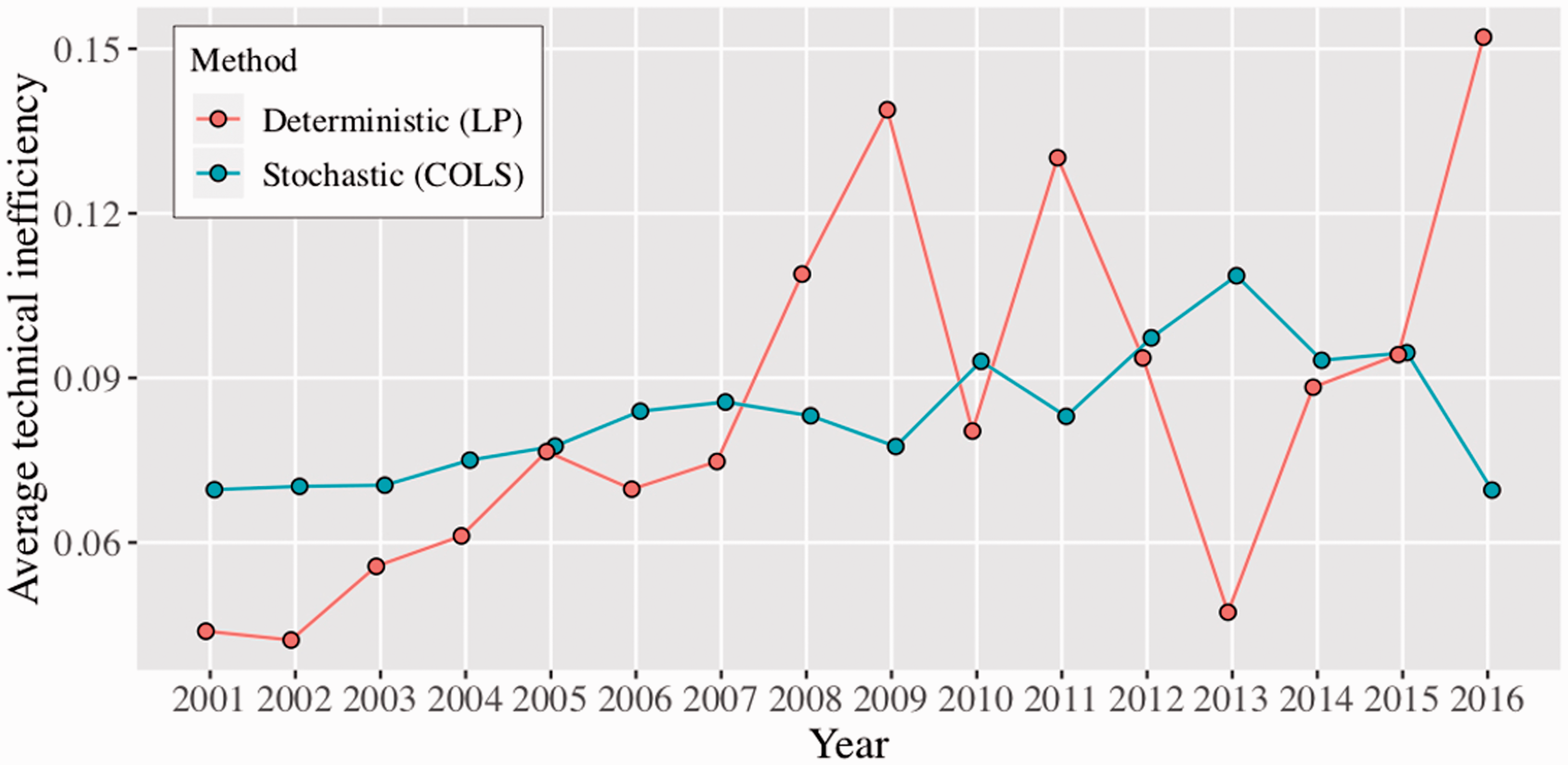
Annual average technical inefficiency over time.

The estimated technical inefficiency enables us to identify the potential slacks for (un)desirable output changes such as extra electricity generation and maximum mitigation of ${CO}_{2}$ . We obtain this by multiplying the technical inefficiency by electricity generation and ${CO}_{2}$ emissions, respectively. Table 6 lists the slack of electricity generation and ${CO}_{2}$ mitigation. Each figure in Table 6 is calculated by summing the slacks and the potential mitigation of each GENCO.

Table 6.

Potential slack of electricity generation and mitigation of CO₂.

Year	Electricity generation (TWh)		CO₂ mitigation (mil. CO₂)
Year	LP	COLS	LP	COLS
2001	6.71	11.31	5.04	7.84
2002	6.93	12.05	5.04	8.22
2003	9.39	12.46	6.73	8.60
2004	11.16	15.54	8.02	10.16
2005	14.82	16.15	10.58	10.77
2006	14.25	18.20	10.23	11.96
2007	17.24	20.67	12.83	13.79
2008	25.75	20.17	18.95	13.91
2009	36.30	19.70	28.38	14.29
2010	22.42	26.68	15.72	18.09
2011	37.70	23.35	29.30	16.18
2012	28.48	28.34	22.57	19.14
2013	14.07	33.51	10.78	22.45
2014	25.69	26.07	19.85	18.37
2015	25.96	24.85	19.88	12.83
2016	41.33	19.96	28.08	12.71
Total	338.21	328.99	251.99	219.30

Sources: KEPCO, annual reports of GENCOs and the Greenhouse gas inventory and Research center; Results calculated by the authors.

The Korean GENCOs, if they operate their facilities with full efficiency, could have generated 328.99–338.21 TWh electricity more during the study period. Also, they could have mitigated ${CO}_{2}$ emissions by 219.30–251.99 mil. ${CO}_{2}$ . This estimated ${CO}_{2}$ mitigation is 8.2–9.5% of the total ${CO}_{2}$ emissions of Korean GENCOs, which can dramatically contribute to the ${CO}_{2}$ mitigation goals of Korea.^m Although these results are theoretical values since the business environment varies across GENCOs and unpredictable events are likely to arise, they can be considered in developing policy tools for sustainable productivity of GENCOs.

Shadow price of CO₂

We estimate the shadow price of ${CO}_{2}$ using equation (24) based on the parameter estimates for the LP and COLS. The annual average electricity price is used as the electricity price, $p$ , which was obtained from KEPCO. Figure 3 depicts the shadow price estimation results across the five GENCOs. The average shadow price using the LP was 82,758 $KRW / t {CO}_{2},$ and that of the COLS was 49,830 $KRW / t {CO}_{2}$ , indicating that the LP’s shadow price was higher than the COLS’s by 32,928 $KRW / t {CO}_{2}$ . This gap in the average shadow price predominately originates from the large variation in the shadow price in LP estimates. For the five GENCOs, all LP results show a larger variation compared to the COLS, especially in the case of Namdong. The COLS results do not seem to yield significant differences across the five GENCOs. For the LP results, the average shadow price is highest for Namdong (135,407 $KRW / t {CO}_{2}$ ) and lowest for Jungbu (35,414 $KRW / t {CO}_{2}$ ). COLS results show the highest shadow price for Namdong (67,724 $KRW / t {CO}_{2}$ ) and the lowest shadow price for Dongseo (42,766 $KRW / t {CO}_{2}$ ).

Figure 3.

Average shadow price of CO₂ across GENCOs.

We confirm that these results are reasonable after observing the actual data. After K-ETS was launched in 2015, GENCOs estimated liabilities for GHG emissions, referring to the expected cost of GHG emissions through purchasing required emission allowances beyond their cap in their 2015 and 2016 annual reports. This helps us acknowledge which GENCOs are more and less efficient in terms of ${CO}_{2}$ emission indirectly. Specifically, if a GENCO has high estimated liabilities for GHG emissions, they produce more ${CO}_{2}$ emissions and operate their firms less efficiently. We found that Namdong has the highest estimated liabilities for GHG emissions, while Dongseo has no estimated liability for GHG emissions, which coincides with our analysis. In contrast, Jungbu shows an intermediate level of estimated liabilities for GHG emissions in their annual reports, though its shadow price is one of the lowest among GENCOs.

Figure 4 presents the annual average shadow price. For most time periods, the LP shows a higher shadow price than the COLS, which corresponds to the results discussed earlier. Also, LP results show a larger variation than COLS results over time. Despite these differences, the decreasing and increasing tendencies are similar for the two methods. The two methods generally show a decreasing trend until 2008, and then show an increase until 2011 (LP) and 2012 (COLS). Both methods show the minimum shadow prices in 2016, i.e., 29,722 $KRW / t {CO}_{2}$ (LP) and 34,644 $KRW / t {CO}_{2}$ (COLS). The trend in the average electricity price does not seem to go along with shadow prices, as shown in Figure 4. This finding indicates that electricity price is unlikely to predict the shadow price of ${CO}_{2}$ and we need to estimate DDFs that incorporate the production process involving both electricity generation and ${CO}_{2}$ emissions.

Figure 4.

Annual average shadow price of CO₂ over time.

We compared our results of the estimated shadow price to those of previous studies, as summarized in Table 1. The shadow prices estimated in some prior studies showed large variations ranging from 5 to 105 USD/ $tC O_{2}$ . This variation mainly comes from the coverage of the data set, different empirical methodologies, or the unit/time of analysis. At the country and provincial levels, the shadow price estimates are relatively smaller than those involving plant- and firm-level analyses. For example, the country-level study of Maradan and Vassiliev³³ and the province-level study of Choi et al.¹⁵ show relatively small values ($0.6–5.2 and $7.2).

Additionally, the shadow price estimates of this study are relatively larger than those of previous studies on Korean electricity generation, such as Kwon and Yun,²⁰ Park and Lim,¹² Lee,⁵ and Lee et al.¹⁰ The main reason for this difference is the unit of analysis. Previous studies mostly use plant-level data while our study adopts firm-level data. The firm-level investigation involves not only the agglomeration of plants but also bureaucratic and administrative characteristics, which plant-level studies cannot capture. Firm-level characteristics are likely to increase inefficiencies within the firm, and subsequently, increase the ${CO}_{2}$ shadow price.

Conclusion and policy implication

We investigated the technical inefficiency and shadow price of ${CO}_{2}$ for Korean fossil-fuel GENCOs during 2001–2016. We used a firm-level data set for the empirical investigation and employed both a deterministic linear programming method (the LP) and a stochastic regression method (the COLS) to obtain robust empirical results.

The empirical results are summarized as follows. First, although there are differences between the two estimation methods, the average technical inefficiency level ranged from approximately 0.083–0.085. This result implies that Korean GENCOs endeavor to use their physical and human resources efficiently to generate electricity. However, the annual trends of technical inefficiency showed discrepancies between the two estimation models. Second, the average shadow price of ${CO}_{2}$ was 118,810 $KRW / t {CO}_{2}$ drawn from the deterministic approach and 71,410 $KRW / t {CO}_{2}$ drawn from the stochastic approach. The shadow price estimations using the LP and the COLS lead to variations across firms. Furthermore, the results of LP show a large variation in the shadow price, while the COLS yields more moderate volatility. The reason for this difference is that the LP does not consider some random errors while the COLS accounted for all errors. The estimated values for the shadow price peak in 2011 (LP) and 2012 (COLS). The average annual electricity price does not correspond to the shadow price. Finally, results show that there is a variation in the shadow price of ${CO}_{2}$ across GENCOs.

The Korean government set the GHG reduction target of 37% below BAU by 2030. The estimate of the required amount of mitigation in emissions to meet this goal is between 219.30–251.99 mil. (or, 8.2–9.5% of total emissions for the five Korean GENCOs). This mitigation will contribute to the sustainability of Korea. Based on our experiments, it can be argued that the level of inefficiency of Korean fossil-fuel generation companies was very low, and their improvement was relatively good. However, policymakers still need to provide strong incentives to reduce inefficiency and potentially benefit from further voluntary emission reductions.

In January 2019, the auction for GHG emission allowances was introduced in Korea based on the K-ETS, and a total of 5.5 mil. ${CO}_{2}$ in allowances were traded. Seven companies participated in the auction with the bidding price ranging from 23,100 KRW to 27,500 KRW. Bidding totaled 10.7 mil. ${CO}_{2}$ . Four companies eventually made successful bids totaling 5.5 mil. ${CO}_{2}$ and the final bid price was 25,500 KRW, which was applied to all transactions for the four companies. The auction has been held monthly since, and its price reached 39,000 KRW as of February 2020. This policy can contribute to improving the liquidity of the emission trading market. We estimated the shadow price of ${CO}_{2}$ emissions as ranging from 29,722 to 34,644 $KRW / t {CO}_{2}$ in 2016. This implies that we found reasonable estimates while the prior literature on Korean fossil-fuel electricity generation estimated a relatively lower shadow price.^5,10,12 In addition, previous studies mostly used plant-level data, but our study was able to achieve more reasonable estimates by adopting firm-level data. This is because firm-level investigation includes not only the agglomeration of plants but also bureaucratic and administrative characteristics that plant-level studies cannot capture.^5,10,12

Our firm-level results can offer more insights on climate change policy. First, there is still the opportunity of reducing ${CO}_{2}$ emissions while maintaining desirable outputs at the national level. Policymakers can provide other incentives to reduce ${CO}_{2}$ emission by adjusting operation levels of GENCOs. Second, firms can discover new business opportunities in the new policy regime. For example, GENCOs with low CO₂ shadow price can employ entrepreneurial strategies by utilizing their sophisticated emission abatement technologies. Finally, policymakers will need to develop carbon reduction technologies by strengthening technological innovation and financial support for energy-related research.³⁴ As such, our analysis suggests the possibility of efficiently allocating carbon savings within Korean fossil-fuel generation companies.

If we obtain more recent data, the two methods are believed to predict more reliable results, and shadow price volatility will allow us to discuss the in depth impacts of market or government regulations. For example, Korea has carried out the first plan of the emissions trading scheme from 2015 to 2017 and is currently carrying out the second plan (2018–2020). In the first plan, the allowance of GHGs was without any charge while the second plan introduced paid allowances. If we could obtain the latest data, the shadow prices for the first and the second planning periods could be compared to provide implications for the subsequent third plan.

We derived an approximation of the allowable CO₂ emissions price in the emission trading market from an economic perspective. Although we attempted to obtain robust empirical results using two parametric approaches, we would like to suggest some words of caution because genuine random errors are not considered in our models. We attempted to apply the stochastic frontier model with random error and inefficiency terms in the estimation process, but the estimation results indicate that the stochastic frontier model is not appropriate. This result is because most DMUs are located on or near the production frontier. To correct this problem, we applied a corrected ordinary least square (COLS) model. In the COLS procedure, however, any residuals are transformed into technical inefficiency, which is a drawback of the COLS. This also requires us to develop an advanced econometric model that utilizes a data set mainly consisting of efficient producers. For example, Song et al.³⁵ addressed the estimation of parametric stochastic models, particularly in the presence of very high- or low-performing observations, which can be outliers due to measurement errors or atypical observations drawn from the tails of an underlying distribution. As our data has several outliers especially due to the data gathering process, it is highly likely that the most advanced methods could yield more robust estimation results. These kinds of advanced econometric models may contribute to solve aforementioned problem. It should be considered in future studies.

Footnotes

Declaration of conflicting interests

The authors declared no potential conflicts of interest with respect to the research, authorship, and/or publication of this article.

Funding

The authors disclosed receipt of the following financial support for the research, authorship and/or publication of this article: Hyundo Choi was supported by the Dongguk University Research Fund of 2019.

ORCID iD

Hyundo Choi

Notes

Dong-Hyun Oh is an Associate Professor in the Department of Industrial Engineering at Inha University. His research interest includes productivity/efficiency change from the perspective of industrial organization. He is also interested in productivity growth of energy and healthcare sectors. His most recent research is published in Journal of Productivity Analysis, Energy Economics, Empirical Economics, and among others.

JongWuk Ahn is an Associate Research Fellow at KRIHS, a think tank of national territorial planning and development in Korea. He worked as a research professor in the Innovation Management Institute at KOREATECH. He is interested in industrial policy and sustainable growth.

Sinwoo Lee is a PhD student at Inha University in Incheon, Korea. He earned a master's degree from Inha University. His research is about productivity and efficiency.

Hyundo Choi is an Associate Professor at Dongguk University – Seoul in Korea. After earning his doctoral degree from Seoul National University, he worked as a postdoctoral fellow at the Belfer Center in Harvard Kennedy School. His research is concerned with technological innovation, organizational learning, and sustainability.

References

KEPCO. Statistics of electric power in Korea. Technical Report, Korea Electric Power Corporation, Korea, 2017.

Lee

Zhou

Directional shadow price estimation of CO2, SO2 and NOx in the United States coal power industry 1990–2010. Energ Econ 2015; 51: 493–502.

World Bank. DataBank microdata data catalog. Report, World Bank, Washington, DC, 2017.

Greenhouse Gas Inventory and Research Center. Second biennial update report of the Republic of Korea: under the United Nations framework convention on climate change. Report, The Government of the Republic of Korea, Korea, 2017.

Lee

Potential cost savings from internal/external CO2 emissions trading in the Korean electric power industry. Energy Policy 2011; 39: 6162–6167.

Coase

RH.

The problem of social cost. J Law Econ 1960; 3: 1–44.

Enerdata. Global Energy Statistical Yearbook 2017. Report, Enerdata, France, 2017.

Matsushita

Yamane

Pollution from the electric power sector in Japan and efficient pollution reduction. Energ Econ 2012; 34: 1124–1130.

Lee

Park

Kim

TY.

Estimation of the shadow prices of pollutants with production/environment inefficiency taken into account: a nonparametric directional distance function approach. J Environ Manage 2002; 64: 365–375.

10.

Lee

JD.

A new approach to measuring shadow price: reconciling engineering and economic perspectives. Energy Econ 2014; 46: 66–77.

11.

Zhou

Fan

Zhou

Marginal CO2 abatement costs: findings from alternative shadow price estimates for Shanghai industrial sectors. Energy Policy 2015; 77: 109–117.

12.

Park

Lim

Valuation of marginal CO2 abatement options for electric power plants in Korea. Energy Policy 2009; 37: 1834–1841.

13.

Huo

Ren

Cai

, et al. The total-factor energy productivity growth of China’s construction industry: evidence from the regional level. Nat Hazards 2018; 92: 1593–1616.

14.

LC.

Evaluating the energy efficiency of European Union countries: the dynamic data envelopment analysis. Energy Env 2019; 30: 27–43.

15.

Choi

Zhang

Zhou

Efficiency and abatement costs of energy-related CO2 emissions in China: a slacks-based efficiency measure. Appl Energy 2012; 98: 198–208.

16.

Zhou

Marginal abatement cost, air pollution and economic growth: evidence from Chinese cities. Energy Econ 2020; 86: 104658.

17.

Lee

Zhang

Technical efficiency, shadow price of carbon dioxide emissions, and substitutability for energy in the Chinese manufacturing industries. Energy Econ 2012; 34: 1492–1497.

18.

Lee

Allocative efficiency, potential cost savings, and power supply price markdown in Korean electric power sector. Energy Env 2019; 30: 617–628.

19.

Choi

Analysis of product efficiency of hybrid vehicles and promotion policies. Energy Policy 2010; 38: 2262–2271.

20.

Kwon

Yun

WC.

Estimation of the marginal abatement costs of airborne pollutants in Korea’s power generation sector. Energ Econ 1999; 21: 545–558.

21.

Murty

Kumar

Dhavala

KK.

Measuring environmental efficiency of industry: a case study of thermal power generation in India. Env Resour Econ 2007; 38: 31–50.

22.

Rezek

Campbell

RC.

Cost estimates for multiple pollutants: a maximum entropy approach. Energy Econ 2007; 29: 503–519.

23.

Gupta

Cost of reducing greenhouse gas emissions: a case study of India’s power generation sector. Report, NOTA DI LAVORO 147, Milano, 2006.

24.

Färe

Grosskopf

Noh

, et al. Characteristics of a polluting technology: theory and practice. J Econom 2005; 126: 469–492.

25.

Simar

Detecting outliers in frontier models: a simple approach. J Prod Anal 2003; 20: 391–424.

26.

Aigner

Chu

SF.

On estimating the industry production function. Am Econ Rev 1968; 58: 826–839.

27.

Chambers

Chung

Färe

Profit, directional distance functions, and Nerlovian efficiency. J Optimiz Theory App 1998; 98: 351–364.

28.

Shephard

RW.

Theory of cost and production functions. Princeton studies in mathematical economics. Princeton: Princeton University Press, 1970.

29.

Coggins

Swinton

JR.

The price of pollution: a dual approach to valuing SO2 allowances. J Environ Econ Manag 1996; 30: 58–72.

30.

Swinton

JR.

At what cost do we reduce pollution? Shadow prices of SO2 emissions. Energy J 1998; 19: 63–83.

31.

Olivier

Janssen-Maenhout

Peters

JA.

Trends in global CO2 emissions. Report, Netherlands Environmental Assessment Agency, The Hague; European Commission, Joint Research Centre (JRC), Institute for Environment and Sustainability (IES), 2016.

32.

Kumbhakar

Lovell

Stochastic frontier analysis. New York: Cambridge University Press, 2000.

33.

Maradan

Vassiliev

Marginal costs of carbon dioxide abatement: empirical evidence from cross-country analysis. Swiss J Econ Stat 2005; 141: 377–410.

34.

Huo

Cai

, et al. Exploring the impact of urbanization on urban building carbon emissions in China: evidence from a provincial panel data model. Sustain Cities Soc 2020; 56: 102068.

35.

Song

Kang

Robust estimation in stochastic frontier models. Comput Stat Data Anal 2017; 105: 243–267.

Measuring technical inefficiency and CO 2 shadow price of Korean fossil-fuel generation companies using deterministic and stochastic approaches

Abstract

Keywords

Introduction

Literature review

Methodology

Underlying assumptions

Directional distance function, inefficiency and shadow price

Estimation of shadow price

Data

Empirical results

Estimation results

Technical inefficiency

Shadow price of CO2

Conclusion and policy implication

Footnotes

Declaration of conflicting interests

Funding

ORCID iD

Notes

References

Shadow price of CO₂