Ineffectiveness of carbon cap-and-trade market

Abstract

Under neoclassical assumptions, this paper develops a model to illustrate the effects of government use of carbon allowances for carbon emission control. We find that control using the instrument of issuing long-term carbon allowances does not produce the same good results in the Decentralised Equilibrium as in the Planning Problem. Thus, while Coase's Theorem ensures that the Pareto optimum is maintained in an economy with multiple agents, it does not align the social development with the economic optimum of the planner. We believe this is due to the that the price of carbon allowances is determined by asset profiles of investors rather than externalities. The steady-state under the special pathway shows that consumption is determined by the rate of technological progress, the total amount of carbon dioxide at steady-state, the level of technology at which steady-state is reached and the total amount of carbon allowances remaining. The comparison with the optimal tax path reveals that the price of carbon allowances has increased too quickly, leading to excessive consumption of fossil fuels in the early stages.

Keywords

climate change optimal policy externality carbon allowance

Introduction

In recent years, as the problem of global warming continues to worsen, the issue of how to reduce greenhouse gas emissions (especially carbon dioxide) has become one of the primary concerns in the world. It's important to discuss the effectiveness of carbon trading markets as a widely used means of reducing emissions and how carbon allowances are allocated.

There is a wealth of research on the effectiveness of carbon allowances at rest¹. Tybout⁴ and Frech III⁵ discuss the effectiveness of the Coase's Theorem in addressing pollution externalities in a non-dynamic context, but neither considers the need for the ’future’ to pay for present decisions in long-run dynamic equilibrium nor does the subject consider only between. Jouvet et al.⁶ showed that there is unique management of permits such that the equilibrium coincides with the optimal path: all permits should be auctioned, i.e. no permits should be given to firms, which is in contradiction with the usual practice of grandfathering. This article demonstrates that the government determines the allowances that should be issued and that firms need to use them in the current period in order for the path of economic development to be optimal. The aforementioned literature has addressed the validity of Coase's Theorem when there is no need to consider emissions at different times or when the government sets the emissions for each period.

In fact, the EU ETS, the Chinese pilot and the Japanese carbon allowance market are managed in such a way as to allow carbon allowances to be fulfilled over an extended period of time, with investors holding carbon allowances being able to choose when to sell them. Therefore, studying how carbon allowances in force over time affect emissions overtime could help governments to adjust their carbon allowance systems.

However, we find that there is less theoretical literature available that discusses the theoretical basis of the Coase's Theorem under cap-and-trade and with allowances that can be used in the long run. This paper analyses, through a dynamic stochastic general equilibrium model, when considering the long-term problem, the market may not allow the economy to move spontaneously towards an optimal path if carbon allowances are marketed as an asset and investors can decide when to sell them. In addition to this, our findings provide a new framework and a simple theoretical basis for the discussion of the validity of Coase's Theorem in carbon markets.

The paper is organised as follows: Section 1 introduces the initial purpose of our exploration of the problem. Section 2 introduces the links between our research and the literature. Section 3 presents some of the foundational settings of the model in this paper, and these assumptions will play a foundational role in the rest of the paper. The form of the production function in the model, the content of the industries covered, and the various model structure settings can have a non-trivial outcome on the final results of the model. There is also a part of our model that deals with the natural science carbon cycle. This part mostly follows the settings of Nordhaus;^7,8 Golosov et al.⁹ However, where we differ from previous literature settings and where we are innovative is in splitting the equation of motion for carbon dioxide into two, making it easier to optimise the use of Bellman's method in the calculations. In Section 4, we present the design and optimal results of the Planning Problem and translate them into a dynamic process. In Section 5, we present general equilibrium results with one representative consumer and two representative firms. In Section 6, we compare the dynamic process of the Planning Problem in Section 4 with the Decentralized Equilibrium results in Section 5 and find that most of the equations of motions are consistent except that in the Decentralized Equilibrium, the movement of the carbon allowance price is determined by the pricing kernel rather than the magnitude of the externality.

In Section 7, we explore an equilibrium under a particular path.² The effect of technological progress on steady-state consumption is positive, but there is an upper limit to this effect. Even if technological progress is very rapid, since we assume that economic growth cannot be completely freed from carbon emissions, the highest steady-state consumption is only that corresponding to the consumption of almost all the carbon allowances in the period when steady-state is reached. The impact of the remaining carbon allowances at the time of reaching steady-state has an incremental positive effect on steady-state consumption. This implies that fighting for more carbon allowances in international negotiations will not only affect the path towards steady-state but will also affect the value of steady-state. The stock of $C O_{2}$ at steady-state has an approximately linear negative effect on steady-state consumption. At the same time, the level of technology at the time of reaching steady-state also has an incremental positive effect on steady-state. In Section 8, we explore the relationship between the movement price of carbon allowances and the optimal carbon tax on the basis of Nordhaus,¹² Stern and Stern¹³ and Nordhaus.⁸ Even at a return level of 5% (the annualised return on carbon allowances in the third phase of the EU ETS is around 20%), the price of carbon allowances still increases much faster than the optimal carbon tax in the long run. This suggests that a long-term carbon allowance market can lead to excessive early consumption of carbon allowances across the economy compared to the optimal path. In Section 9, we summarise the results of the model and describe the mechanisms that give rise to the problem.

Literature review

The ideological basis of this paper can be traced back to the discussion of the externalities generated by environmental pollution. The concept of externality was first developed by economist Arthur Pigou in the 1920s, seeing in Pigou.¹⁴ According to Griffin and Steele,¹⁵ external costs exist when "the private calculation of benefits or costs differs from society's valuation of benefits or costs". Dolbear¹⁶ pointed out that the occurrence of an external diseconomy will lead to a discrepancy between marginal social net benefit and cost Environmental pollution clearly creates externalities, as the damaging consequences of pollution are borne by society as a whole but are not reflected in market transactions³.

In order to solve the problem of externalities, two instruments Tax, Emission Allowance began to be widely discussed and used. The idea of taxing externalities comes from the idea of taxing the excess benefits received by firms, which was one of the solutions given by Pigou in 1920 when he discussed externalities subsidising positive externalities and taxing negative externalities by an amount exactly equal to the difference between marginal net private output and marginal net social output.

There is rich theoretical literature on the issue of carbon taxation⁴.

Many kinds of literature focus on the determination of the optimal carbon tax, and the model settings used in our paper draw in part on the capital, resource and pollution run-up settings used in the optimal carbon tax discussion⁵.

Another way to address the externality is through market trading of emission rights, which has the advantage of not requiring a direct carbon tax rate from the social planner, avoiding the above problem of the difficulty of accurately measuring the optimal carbon tax. The most fundamental economic theory of carbon trading is Coase's Theory of externalities and property rights, Coase²⁷ points out that Pigou's solution is difficult to implement. Dales²⁸ introduced the concept of property rights to the control of pollution emissions for the first time. He defined ’emission rights’ as the right of a right holder to emit pollutants into the environment under legally defined conditions, and if trading of this right is allowed under certain conditions, the market can be used to achieve the most efficient emission reduction outcome. Emissions trading as an instrument has received more widespread attention in recent years. Under the Kyoto Protocol and the subsequent Paris Agreement, carbon trading has become a hot topic of research and focus.

The question of which is the better means of controlling carbon emissions, a carbon tax or tradable carbon allowances is still a controversial one⁶. From the point of view of Coase's theorem, the emergence of carbon credits has served as a means of identifying rights and helping the market to achieve optimality.

It is also difficult to trust complex models to obtain a reasonable carbon price because of the greater error and uncertainty associated with complex systems, so expectations of a reasonable carbon price become more difficult to trade-off when different models derive different results⁷.

The diversity of estimates shows that estimating a reasonable carbon tax is a controversial and difficult task.

Nordhaus⁷ compares the carbon tax and carbon allowance options in a more systematic way. And mentions Weitzman³⁴ in the comparison and explains that price regulation is more effective if the costs are highly non-linear compared to the benefits; conversely, if the benefits are highly non-linear and the costs are close to linear, quantity regulation (carbon allowance system) is more effective. At the same time, a carbon allowance system can be more damaging to the economy due to the highly volatile price of carbon dioxide. And the double dividend from environmental taxation would mitigate the losses from other taxes, seeing Bovenberg and Goulder²⁹ and Goulder et al.³¹. Parry³² explores the advantages and disadvantages between retrospective, auctioned carbon credits and carbon taxes in terms of the mechanism of the impact on labour, and argues that carbon taxes and auction methods are preferable given the distortive nature of the tax system and the fact that auction proceeds and carbon tax revenues can mitigate distortions to some extent. Whereas Zakeri et al.³⁶ argue that in numerical simulations, the trend of carbon emission reduction is unstable and non-linear as the price of carbon steadily increases and that the increase in carbon transaction costs is also non-linear, so a carbon tax may be more favourable from an uncertainty point of view. Mathys and de Melo³³ argue that a carbon tax is a more efficient option than the current way of trading carbon emissions, but that does not mean that a more efficient carbon trading option does not exist And a tradable approach to carbon credits could help the capital flow from rich to poor countries. Parker³⁵ refers to carbon credits and carbon taxes as quantitative and price-based instruments and shows that in an ideal state of complete information, the government could achieve the same optimal outcome with either of these and that the essential trade-off between the two options lies in the trade-off between total emissions and costs. Elkins and Baker³⁰ systematically describes the literature and examples on carbon taxes and carbon permits and sets out the theoretical underpinnings of these conclusions.

Our article offers a new perspective on the trade-offs between carbon taxes and carbon allowances. According to the conclusions of our article, a carbon tax is likely to be more beneficial than carbon trading in the long run, solely from the perspective of achieving optimality for social planners.

Guided by Coase's theorem, the carbon markets in China and the European Union provide companies with freely tradable carbon allowances that they can use at their own discretion. To some extent, governments believe that these carbon allowances will put the economy on a good path. However, our research has demonstrated that time-of-use free carbon allowances can be depleted too quickly. In contrast to this policy, if the government reintroduces a carbon tax each year or does not allow carbon allowances to be used across time, the economy has the opportunity to converge towards the optimal path.

The most relevant recent study to our research is how the carbon market has affected the economy and carbon emissions. Zhang et al.³⁸ estimate the impact on the economy under different carbon quota allocation methods in the Chinese carbon market. Yu et al.³⁹ described how different industries and provinces are affected under carbon allowance policies. Yu et al.³⁹ found that the existence of carbon allowances effectively curbs carbon emissions. Although the economy was affected to some extent, the industry did generate a reasonable trade-off. Forbes and Zampelli⁴⁰ estimate the significant contribution of wind energy and carbon markets to carbon dioxide emissions reductions. These studies, previous studies and our own, clearly show that carbon allowance policies can indeed be effective in reducing carbon dioxide emissions. And again, Forbes and Zampelli⁴⁰ recall that carbon markets are effective under static conditions. However, due to national implementation issues, carbon allowances can often be used at different times. Whether the carbon allowance market is efficient under dynamics remains a question that needs to be examined. The salient contribution of our model is to show that the use of carbon allowances to allocate carbon emissions in dynamic time is ineffective.

A general assumption of the economy and the climate

In this section, we describe the general settings in the model that will come into play in Section 4, Section 5 and Section 6. We apply the framework in Golosov et al.⁹ to the analysis of the validity of carbon allowances. In particular, our proof does not need to rely on a particular form of the utility function and the production function, but only on the assumption of the homogeneous function of the production function.

We consider a neoclassical growth model with two sectors. Time is discrete and infinite.

There is a representative household with the utility function (C is the consumption, and $β \in (0, 1)$ is the discount factor) :

E_{0} \sum_{t = 0}^{\infty} (β^{t} U (C_{t}, 1 - L_{t}),

(1)

where U is a standard concave period utility function.

The production process consists of two components, the producer of energy and the producer of the final product. The output constraint on the final product is (to simplify the model, we have not considered capital depreciation):

C_{t} + K_{t + 1} = Y_{t} + K_{t} .

(2)

The left-hand side of the equation is the consumption of resources and the capital stock for the next period. The first term on the right-hand side,

Y_{t}

, is the final product output and the second term is the capital in the current period.

The output of the final product is portrayed by the production function of the first production sector:

Y_{t} = F_{1} (K_{1, t}, L_{1, t}, E_{t}, S_{t}, z_{t}) and z_{t + 1} = F_{z} (z_{t}, ϵ_{t}) .

(3)

The arguments of

F_{1, t}

include the standard inputs

K_{1, t}

and labour of

L_{1, t}

(this production sector uses capital and labour), and the energy of

E_{t}

z_{t}

denotes the possibility of technological development and changes in production patterns in the course of economic development. This change may come from a number of sources. For example, it may be an increase in the use of energy, a continuous improvement in production technology or an increase in the use of capital, etc.

F_{z}

is the motion function of z, and

ϵ_{t}

is the exogenous stochastic shock.

Finally, we need to highlight the impact of the climate variable $S_{t}$ on the production of the final product. In fact, the effect of $S_{t}$ on the production of final goods may be positive or negative. For example, an increase in the concentration of carbon dioxide may increase food production, while an increase in the concentration of carbon dioxide and consequently warming may also reduce the labour capacity of workers. In colder regions, however, warming may increase the labour productivity of local workers over the year. The climate variable $S_{t}$ can be more than just carbon dioxide concentration; it can be methane concentration, nitrogen oxide concentration, temperature and even precipitation, all of which can be influenced by human activity. In this paper, however, the focus is on carbon dioxide emissions. At the same time, the potential catastrophe of increasing carbon dioxide concentrations has received a great deal of attention from the academic community, so here we are looking at the negative externalities of carbon dioxide emissions.

Our assumption that $S_{t}$ affects production only is made mainly so as to make our analysis closer to, and easier to compare with Golosov et al.,⁹ Nordhaus's RICE and DICE treatments.

Next, we turn to the second production sector: the production of energy.

E_{t} = F_{2} (K_{2, t}, L_{2, t}, R_{t}, z_{t}) \geq 0.

(4)

In our production function setting, the production of energy itself requires no energy input. We adopt this assumption on the basis that we do not distinguish between different energy sources. In fact, it is less relevant to our core concern.

In the general setting, it is usually necessary to consider the impact of the continuous extraction of resources (e.g. fossil energy) on the production of energy, and generally to discuss the following resource consumption equation:

R_{t + 1} = R_{t} - E_{t} \geq 0.

(5)

And in our model, again, the resource reserves

R_{t}

are entered into

F_{2}

In each period, the different factors of production are cleared individually.

K_{1, t} + K_{2, t} = K_{t} and L_{1, t} + L_{2, t} = L_{t} .

(6)

Finally, for the motion of

S_{t}

, we refer to the setting in Golosov et al.⁹ and set the carbon dioxide process as follows:

S_{t} = S_{1, t} + S_{2, t},

(7)

S_{1, t + 1} = (1 - ϕ) S_{1, t} + a E_{t},

(8)

S_{2, t + 1} = S_{2, t} + b E_{t} - H_{t} .

(9)

where

ϕ \in (0, 1)

is a geometric rate of remaining share decaying and

H_{t}

is the exogenous carbon reduction, which can be random.

(7) indicates that the carbon in the atmosphere consists of two parts, the first part remaining in the atmosphere for a long time and the other part being in the carbon cycle and decreasing. (8) shows the contribution of carbon emissions involved in the carbon cycle, while (9) shows the carbon emissions that remain in the atmosphere over time. In fact, this assumption is consistent with the setting of Golosov et al.⁹

The planning problem

Next, we solve the Planning Problem, comparing it with market results after obtaining some key equations.

The social planner solves the agent's utility maximization problem: (10)

\max_{{C_{t}, K_{t}, K_{1, t}, K_{2, t}, L_{t}, L_{1, t}, L_{2, t}, E_{t}, R_{t + 1}, S_{1, t + 1}, S_{2, t + 1}}} E_{0} \sum_{t = 0}^{\infty} β^{t} U (C_{t}, 1 - L_{t}),

(10)

subject to (4), (5), (6), (7), (8), (9) and

C_{t} + K_{t + 1} = F_{1, t} (K_{1, t}, L_{1, t}, E_{t}, S_{t}) + K_{t}

(11)

z_{t + 1} = F_{z} (z_{t}, ϵ_{t})

(12)

as well as nonnegativity constraints.

C_{t} + K_{t + 1} = F_{1} (K_{1, t}, L_{1, t}, E_{t}, S_{t}, z_{t}) + K_{t},

(13)

K_{1, t} + K_{2, t} = K_{t},

(14)

E_{t} = F_{2} (K_{2, t}, L_{2, t}, S_{t}, z_{t}),

(15)

L_{1, t} + L_{2, t} = L_{t},

(16)

S_{1, t + 1} = (1 - ϕ) S_{1, t} + a E_{t},

(17)

S_{2, t + 1} = S_{2, t} + b E_{t} - H_{t},

(18)

R_{t + 1} = R_{t} - E_{t},

(19)

U_{C_{t}} F_{1 L_{1, t}} + U_{L_{t}} = 0,

(20)

\frac{U_{C_{t}} F_{1 K_{1, t}} F_{1 L_{2, t}}}{F_{2 K_{2, t}}} + U_{L_{t}} = 0,

(21)

β E_{t} (U_{C_{t + 1}} + U_{C_{t + 1}} F_{1 K_{1, t + 1}}) = U_{C_{t}},

(22)

β E_{t} (U_{C_{t + 1}} F_{1 K_{1, t + 1}} F_{1 S_{1, t + 1}} + (1 - ϕ) λ_{5, t + 1}) = λ_{5, t},

(23)

β E_{t} (U_{C_{t + 1}} F_{1 K_{1, t + 1}} F_{1 S_{2, t + 1}} + λ_{6, t + 1}) = λ_{6, t},

(24)

β E_{t} (\frac{U_{C_{t} + 1} F_{1 K_{1, t + 1}}}{F_{2 K_{2, t + 1}}} F_{2 R_{2, t + 1}} + λ_{7, t + 1}) = λ_{7, t},

(25)

U_{C_{t}} F_{1 E_{t}} - \frac{U_{C_{t}} F_{1 K_{1, t}}}{F_{2 K_{2, t}}} + λ_{5, t} a + λ_{6, t} b - λ_{7, t} = 0.

(26)

The Planning Problem is composed of (13), (14), (15), (16), (17), (18), (19), (20), (21), (22), (23), (24), (25) and (26) consisting of fourteen dynamic equations.

The decentralized equilibrium

The previous section characterized the solution to the Planning Problem and found the optimal dynamic process. In this section, we will explore the optimal path under the Decentralized Equilibrium.

Consumers

Representative consumers maximize their utility function through decisions ( $A_{t}$ is the carbon allowance surplus, and ${\hat{E}}_{t}$ is the carbon allowance use).

\max_{{C_{t}, K_{t}, L_{t}, A_{t}, {\hat{E}}_{t}}} E_{0} \sum_{t = 0}^{\infty} β^{t} U (C_{t}, 1 - L_{t}),

(27)

subject to (

n_{t}

is the remuneration per unit of labour,

p_{t}

is the price of carbon allowances and

r_{t}

is the capital return)

C_{t} + K_{t + 1} = n_{t} L_{t} + p_{t} {\hat{E}}_{t} + (1 + r_{t}) K_{t}

(28)

A_{t + 1} = A_{t} - {\hat{E}}_{t} .

(29)

with the non-negativity condition.

C_{t} + K_{t + 1} = n_{t} L_{t} + p_{t} {\hat{E}}_{t} + (1 + r_{t}) K_{t},

(30)

A_{t + 1} = A_{t} - {\hat{E}}_{t},

(31)

U_{C_{t}} n_{t} + U_{L_{t}} = 0,

(32)

β E_{t} ((1 + r_{t + 1}) U_{C_{t + 1}}) = U_{C_{t}},

(33)

β E_{t} (p_{t + 1} U_{C_{t + 1}}) = p_{t} U_{C_{t}} .

(34)

Consumer choice consists of five dynamic equations (30), (31), (32), (33) and (34).

Producers 1

The decision problem for producer $1$ is a static problem of solving the profit maximization problem (where ${\bar{E}}_{t}$ is the energy and $q_{t}$ is the price per unit of energy) under the assumption of no cost of adjustment capital as (35).

\max_{{K_{1, t}, L_{1, t}, {\bar{E}}_{t}}} E_{t} F_{1} (K_{1, t}, L_{1, t}, {\bar{E}}_{t}, S_{1, t} + S_{2, t}, z_{t}) - r_{t} K_{1, t} - n_{t} L_{1, t} - q_{t} {\bar{E}}_{t}

(35)

The first-order conditions are:

F_{1 K_{1, t}} = r_{t},

(36)

F_{1 L_{1, t}} = n_{t},

(37)

F_{1 {\bar{E}}_{t}} = q_{t} .

(38)

Producers 2

On the other hand, the production of Producers 2 also considers a static problem:

\max_{{K_{1, t}, L_{1, t}}} (q_{t} - p_{t}) F_{2} (K_{1, t}, L_{1, t}, R_{t}, z_{t}) - r_{t} K_{1, t} - n_{t} L_{1, t} .

(39)

The reason for considering the Producers 2 optimisation problem as the static problem is that the discussion in this paper is all about the representative producer, and the individual energy producers being summed do not need to consider the impact of their own extraction behaviour on the total reserves.

The first-order conditions are:

(q_{t} + p_{t}) F_{2 K_{2, t}} = r_{t},

(40)

(q_{t} + p_{t}) F_{2 L_{2, t}} = n_{t},

(41)

Market clearance

Firstly this section is still consistent with factor market clearing (6), except that it should be noted that energy supply clearing is:

{\hat{E}}_{t} = F_{2} (K_{2, t}, L_{2, t}, R_{t}, z_{t}) = {\bar{E}}_{t} .

(42)

The difference between the planning problem and the decentralized equilibrium

Next, the optimal result in the Planning Problem is denoted by the shape $C_{t}^{*}$ , and the optimal result in the Decentralized Equilibrium is denoted by the shape $C_{t}^{* *}$ .

Though (20) and (21), we have

F_{1 K_{1, t}^{* *}} = \frac{F_{2 K_{2, t}^{* *}}}{F_{2 L_{2, t}^{* *}}} F_{1 L_{2, t}^{* *}} .

(43)

With (36),(37), (40) and (41), we deduce

F_{1 K_{1, t}^{*}} = \frac{F_{2 K_{2, t}^{*}}}{F_{2 L_{2, t}^{*}}} F_{1 L_{2, t}^{*}} .

(44)

(43) and (44) represent the Euler equations for the capital and labour factors. It reflects the marginal substitution relationship between the different factors of production of the two producers.

(13) is

C_{t}^{* *} + K_{t + 1}^{* *} = F_{1} + K_{t}^{* *} .

(45)

From the neoclassical assumption that product profit is

0

, by (30), (35), (39) and (42) we can know that

C_{t}^{*} + K_{t + 1}^{*} = F_{1} + K_{t}^{*} .

(46)

(45) and (46) are the aggregate capital movement equations under the societies of the two regimes, and the Decentralized Equilibrium is the more intuitive result under the premise that the manufacturer's profit is

0

(20) implies

U_{C_{t}^{*}} F_{1 L_{1, t}^{*}} + U_{L_{t}^{*}} = 0.

(47)

(125), (126) and (37) implies

U_{C_{t}^{* *}} F_{1 L_{1, t}^{* *}} + U_{L_{t}^{* *}} = 0.

(48)

(47) and (48) are results induced by the Euler equation for consumer choice, showing that the consumer's substitution relationship between capital and leisure is equivalent under both regimes.

(22) implies

β E_{t} (U_{C_{t + 1}^{*}} + U_{C_{t + 1}^{*}} F_{1 K_{1, t + 1}}^{*}) = U_{C_{t}^{*}} .

(49)

(33) and (36) means

β E_{t} (U_{C_{t + 1}^{* *}} + U_{C_{t + 1}^{* *}} F_{1 K_{1, t + 1}}^{* *}) = U_{C_{t}^{* *}} .

(50)

(49) and (50) are pricing equations for the rate of return on capital, which represent that there is the same form of the pricing kernel under both paths.

The process of capital movement and the conditions for liquidation are next to be considered.

The Decentralized Equilibrium

K_{1, t}^{*} + K_{2, t}^{*} = K_{t}^{*},

(51)

E_{t}^{*} = F_{2} (K_{2, t}^{*}, L_{2, t}^{*}, S_{1, t}^{*} + S_{2, t}^{*}, z_{t}),

(52)

L_{1, t}^{*} + L_{2, t}^{*} = L_{t}^{*},

(53)

S_{1, t + 1}^{*} = (1 - ϕ) S_{1, t}^{*} + a E_{t}^{*},

(54)

S_{2, t + 1}^{*} = S_{2, t}^{*} + b E_{t}^{*} - H_{t},

(55)

R_{t + 1}^{*} = R_{t}^{*} - E_{t}^{*} .

(56)

The Decentralized Equilibrium:

K_{1, t}^{* *} + K_{2, t}^{* *} = K_{t}^{* *},

(57)

E_{t}^{* *} = F_{2} (K_{2, t}^{* *}, L_{2, t}^{* *}, S_{1, t}^{* *} + S_{2, t}^{* *}, z_{t}),

(58)

L_{1, t}^{* *} + L_{2, t}^{* *} = L_{t}^{* *},

(59)

S_{1, t + 1}^{* *} = (1 - ϕ) S_{1, t}^{* *} + a E_{t}^{* *},

(60)

S_{2, t + 1}^{* *} = S_{2, t}^{* *} + b E_{t}^{* *} - H_{t},

(61)

R_{t + 1}^{* *} = R_{t}^{* *} - E_{t}^{* *} .

(62)

(34), (36) and (40) implies

β E_{t} ([\frac{F_{1 K_{1, t + 1}^{* *}}}{F_{2 K_{2, t + 1}^{* *}}} - F_{1 E_{t + 1}^{* *}}] U_{C_{t + 1}^{* *}}) = (\frac{F_{1 K_{1, t}^{* *}}}{F_{2 K_{2, t}^{* *}}} - F_{1 E_{t}^{* *}}) U_{C_{t}^{* *}} .

(63)

This equation is essentially the pricing equation for carbon allowances, $(\frac{F_{1 K_{1, t}^{* *}}}{F_{2 K_{2, t}^{* *}}} - F_{1 E_{t}^{* *}})$ represents the price of carbon allowances. Unfortunately, in the Planning Problem, we do not get this equation, which shows that the Coase theorem still does not hold unconditionally even in a neoclassical framework. In the Planning Problem, we obtain by (24), (25) and (26)

\begin{aligned} β E_{t} & ([\frac{F_{1 K_{1, t + 1}^{*}}}{F_{2 K_{2, t + 1}^{*}}} - F_{1 E_{t + 1}^{*}}] U_{C_{t + 1}^{*}} + a ϕ λ_{5, t + 1}^{*} \\ + [F_{1 K_{1, t + 1}^{*}} (a F_{1 S_{1, t + 1}^{*}} + b F_{1 S_{2, t + 1}^{*}} - \frac{F_{2 R_{t + 1}^{*}}}{F_{2 K_{2, t + 1}^{*}}})] U_{C_{t + 1}^{*}}) \\ = (\frac{F_{1 K_{1, t}^{*}}}{F_{2 K_{2, t}^{*}}} - F_{1 E_{t}^{*}}) U_{C_{t}^{*}} . \end{aligned}

(64)

The two equilibria have

11

and

12

equations of motion to be solved (in fact the planner economy also requires

λ_{5, t}

for the process of motion)

{C_{t}, K_{t}, K_{1, t}, K_{2, t}, L_{t}, L_{1, t}, L_{2, t}, E_{t}, R_{t + 1}, S_{1, t + 1}, S_{2, t + 1}} .

(65)

11

and

12

processes.

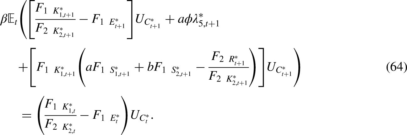
Classical steady-state

In this section, we look at the steady-state analysis of the decentralized equilibrium to explore the economic operation of the carbon allowance system.

In this section, let the utility function take the form:

U (C_{t}, 1 - L_{t}) = \frac{C_{t}^{1 - α_{C}}}{1 - α_{C}} + \frac{{(1 - L_{t})}^{1 - α_{L}}}{1 - α_{L}} .

(66)

According to Golosov et al.,⁹ we assume a production function of Producers 1: (67).

F_{1} (K_{1, t}, L_{1, t}, {\bar{E}}_{t}, S_{1, t} + S_{2, t}, z_{t}) = z_{t} e^{- γ_{t} (S_{1, t} + S_{2, t})} K_{1, t}^{α_{1, K}} L_{1, t}^{α_{1, L}} {\bar{E}}_{t}^{1 - α_{1, K} - α_{1, L}},

(67)

and Producers 2 has no cost to the product, which implies

q_{t} = p_{t}

We assume that at steady-state the air has a steady amount of carbon, the technical setting $H_{t}$ in (9) is to provide the possibility of a steady-state. Let $R a_{q_{t}} = \frac{q_{t + 1}}{q_{t}}$ and the growth rates of the other variables are expressed in the same way. (45) and (67) implies

C = z_{t} e^{- γ S} K^{α_{1, K}} L^{α_{1, L}} E_{t}^{1 - α_{1, K} - α_{1, L}} = F_{1}

(68)

which implies

R a_{z_{t}} = R a_{E_{t}}^{α_{1, K} + α_{1, L} - 1} .

(69)

Then we can deduce that

z_{t} E_{t}^{1 - α_{1, K} - α_{1, L}}

is a constant that does not vary with time. We assume that

z_{t} E_{t}^{1 - α_{1, K} - α_{1, L}} = c_{t e c h}

With (47), we have

C^{- α_{C}} α_{1, L} \frac{C}{L} - (1 - L)^{- α_{L}} = 0.

(70)

(49) is equal to

β (1 + α_{1, K} \frac{C}{K}) = 1.

(71)

(68), (70) and (71) forms a steady-state system. Combine (68), (70), (71) and assumption of

α_{L} = 0

, we have the following solution:

C = {(c_{t e c h} e^{- γ S} {(α_{1, L})}^{α_{1, L}} {[\frac{β α_{1, K}}{1 - β}]}^{α_{1, K}})}^{\frac{1}{1 - α_{1, K} - α_{1, L} (1 - α_{1, L})}},

(72)

L = α_{1, L} C^{1 - α_{C}},

(73)

K = \frac{β α_{1, K}}{1 - β} .

(74)

Then, we have the following classical result.

Proposition 7.1

Consumption in the steady-state depends on the rate of technological progress.

Proof.

We assume that the economy enters a steady-state after period $t_{0}$ , when the level of technology is $z_{t_{0}}$ . The total carbon allowance remaining at this point is $A_{t_{0}}$ . Then we have $\sum_{t = t_{0}}^{\infty} E_{t_{0}} R a_{E}^{t - t_{0}} = A_{t_{0}}$ which implies:

E_{t_{0}} = A_{t_{0}} (1 - R a_{E}) .

(75)

Combine (69), (72), (75) and defination of $c_{t e c h}$ , we have

C = {((z_{t_{0}} A_{t_{0}} (1 - R a_{z}^{\frac{1}{α_{1, K} + α_{1, L} - 1}})) e^{- γ S} {(α_{1, L})}^{α_{1, L}} {[\frac{β α_{1, K}}{1 - β}]}^{α_{1, K}})}^{\frac{1}{1 - α_{1, K} - α_{1, L} (1 - α_{1, L})}} .

(76)

It is easy to see the steady-state value of consumption is determined by the rate of technological growth

R a_{z}

After unitisation, we show the form $C = {(1 - R a_{z}^{\frac{1}{α_{1, K} + α_{1, L} - 1}})}^{\frac{1}{1 - α_{1, K} - α_{1, L} (1 - α_{1, L})}}$ . According to Golosov et al.,⁹ let $α_{1, K} = 0.3$ , $α_{1, L} = 0.66$ and $α_{1, K} + α_{1, L} - 1 = - 0.04$

With Figure 1, it has a greater impact on steady-state consumption when the rate of technological growth is low. And when the rate of technological growth is high, it hardly affects consumption when it increases or decreases. This result is based on the assumption that the economy cannot develop without carbon emissions. Even if technological progress is rapid, the limiting case is that the vast majority of carbon allowances are consumed in the first period after the steady-state is reached. At the current level of technology, the total output does have an upper limit.

Figure 1.

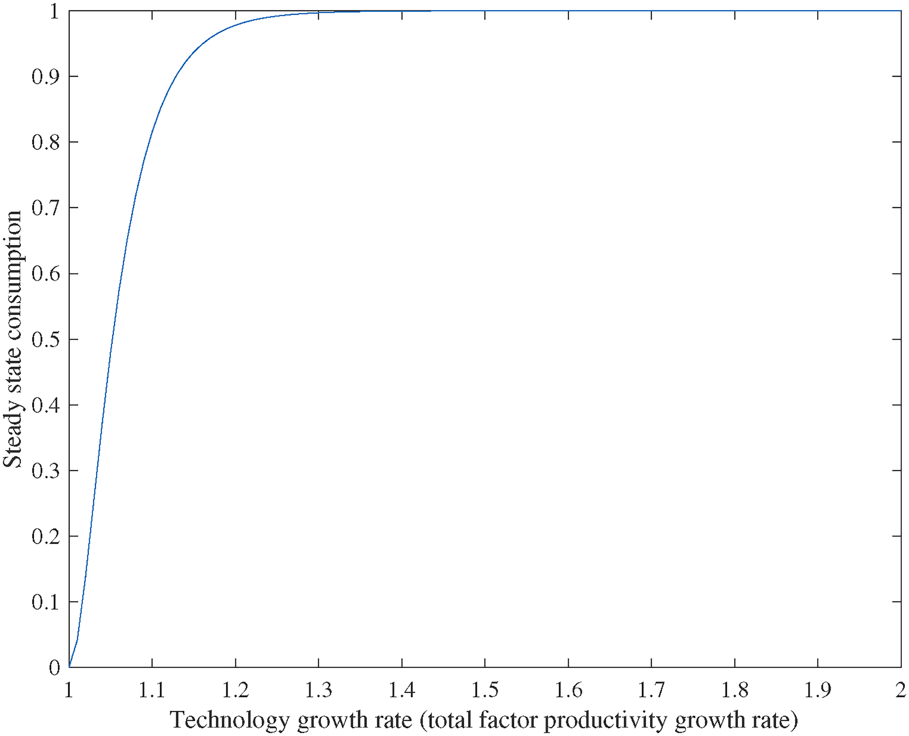
The relationship between steady-state consumption and technological progress.

Through similar discussions of Proposition 7.1, we can see:

Proposition 7.2

Keeping the level of technology and the rate of technological progress constant, the more carbon allowances remaining when the steady-state is reached the higher the steady-state value of consumption.

After unitisation, we show the form $C = (A_{t_{0}})^{\frac{1}{1 - α_{1, K} - α_{1, L} (1 - α_{1, L})}}$ . According to Golosov et al.,⁹ let $α_{1, K} = 0.3$ and $α_{1, L} = 0.66$ .

In Figure 2, the effect of the allowance remaining when steady-state is reached is a downward convex function for steady-state consumption. Proposition 7.2 implies that in the case of multiple countries, each with a closed economy, the allocation of carbon allowances will directly affect the steady-state economy of each country. Further, the international game surrounding the allocation of carbon allowances becomes more important.

Figure 2.

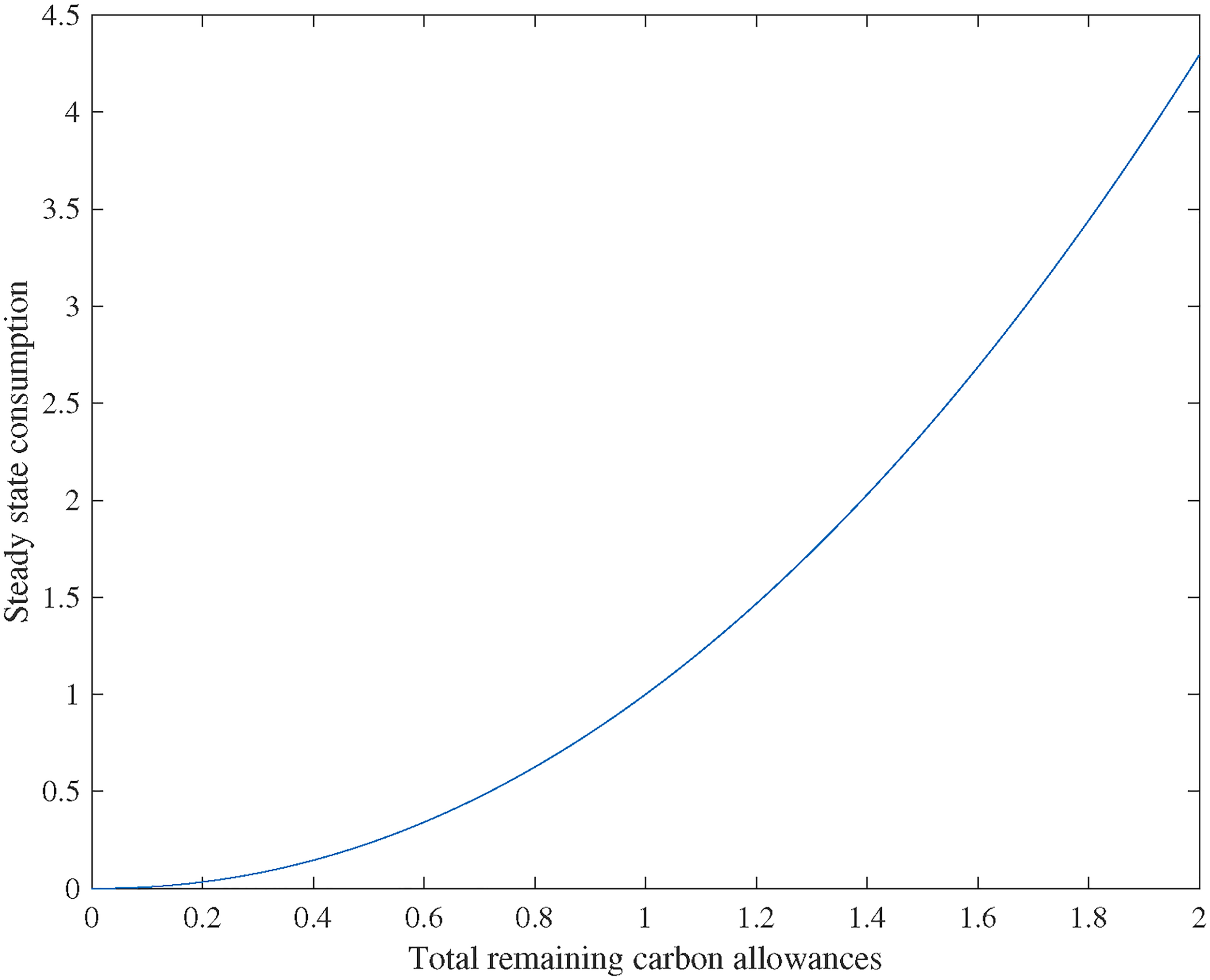
The relationship between steady-state consumption and remaining carbon allowances.

Proposition 7.3

The more stable carbon dioxide in the atmosphere at steady-state, the lower the steady-state consumption value.

After unitisation, we show the form $C = (e^{- γ S})^{\frac{1}{1 - α_{1, K} - α_{1, L} (1 - α_{1, L})}}$ . According to Golosov et al.,⁹ let $γ = 5.3 \times 10^{- 5}$ , $α_{1, K} = 0.3$ and $α_{1, L} = 0.66$ . S is around 800.

According to Figure 3, the amount of atmospheric carbon dioxide in the steady-state damages steady-state consumption in an approximately linear fashion. It is therefore important to set a suitable upper limit for atmospheric carbon dioxide.

Figure 3.

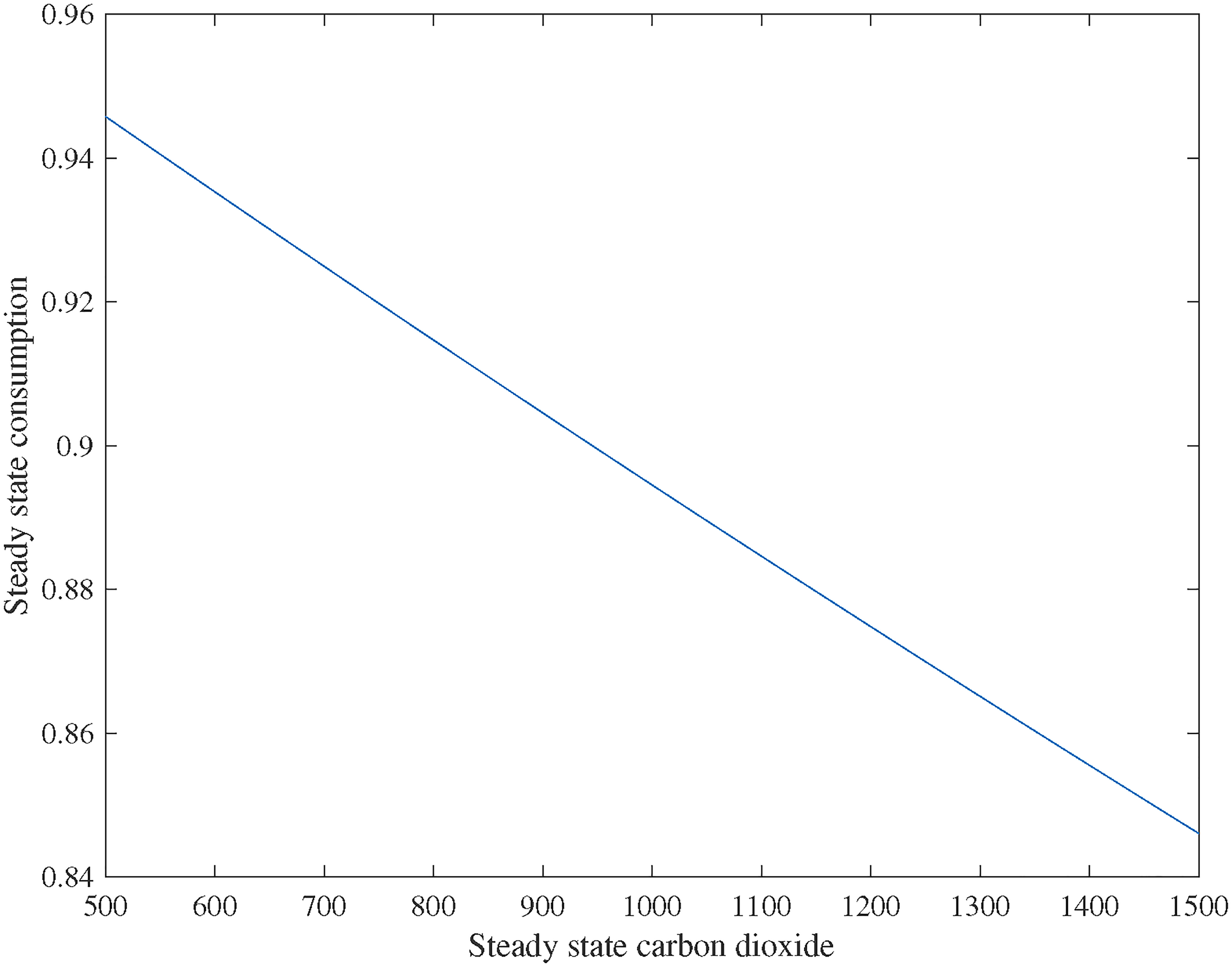
The relationship between steady-state consumption and steady-state carbon dioxide.

Finally, we have:

Proposition 7.4

The higher technology at the beginning of steady-state, the higher the steady-state consumption value.

After unitisation, we show the form $C = (z_{t_{0}})^{\frac{1}{1 - α_{1, K} - α_{1, L} (1 - α_{1, L})}}$ . According to Golosov et al.,⁹ let $α_{1, K} = 0.3$ , $α_{1, L} = 0.66$ and $α_{1, K} + α_{1, L} - 1 = - 0.04$

With Figure 4, consumption at steady-state is incrementally positively related to the level of technology at the start of steady-state.

Figure 4.

The relationship between steady-state consumption and technology at the beginning of steady-state.

By pricing the equation we can also obtain, in steady-state,

\frac{q_{t + 1}}{q_{t}} = \frac{1}{β} = 1 + r_{t}

(77)

which will play an important role in the price measurement of carbon allowances.

Measurement of carbon price

In the Decentralized Equilibrium, with (33), (34) and assumption of $U (C_{t}, 1 - L_{t}) = \frac{C_{t}^{1 - α_{C}}}{1 - α_{C}} + \frac{{(1 - L_{t})}^{1 - α_{L}}}{1 - α_{L}} .$ , we have the following pricing equation:

E_{t} (1 + r_{t + 1}) = \frac{1}{β} - \frac{C O V_{t} (1 + r_{t + 1}, R a_{C_{t}}^{- α_{C}})}{E_{t} (R a_{C_{t}}^{- α_{C}})},

(78)

E_{t} (R a_{q_{t}}) = \frac{1}{β} - \frac{C O V_{t} (R a_{q_{t}}, R a_{C_{t}}^{- α_{C}})}{E_{t} (R a_{C_{t}}^{- α_{C}})} .

(79)

t is difficult to compare which is more correlated with the growth rate of consumption, the rate of increase in the price of carbon allowances or the rate of return on capital. However, during the introduction of the carbon allowance market, the price of carbon allowances has shown fluctuations that far exceed the rate of return on stocks. This fact implies that carbon allowance returns are more likely to have higher rates of return (although in the steady-state (77) the two rates of return exhibit the same properties).

In fact, the price of carbon allowances did show a high rate of increase. In the third phase of the EU ETS (1 January 2013 - 31 December 2020) the price of carbon allowance futures rose from 6.37 to 32.57, an annualised return of 22.6%.

Based on the above analysis, we will examine the movement of carbon prices for different returns and compare them with the results of current carbon price measurements.

According to Table 1 and Figure 5, we base our discussion on the assumption that the price of carbon allowances in 2005 is the same as the optimal carbon tax (in fact, the government can control the price of carbon allowances by regulating the total amount of carbon allowances). It can be seen that the corresponding 2015 carbon allowance prices in the 0.05 to 0.2 range are all higher than the theoretical optimal 2015 carbon price. Even if we ignore the realistic observed level of return of 20%. At a return of around 0.7 alone, the price of carbon allowances is still rising too fast compared to the carbon tax. This is because investors treat carbon allowances as an asset rather than a means of removing externalities. The path of the price movement of carbon allowances is dependent on the investment decisions of investors. Within realistic parameters, the price of carbon allowances is showing a much faster rate of increase than the optimal carbon tax. This will lead to an entire economy consuming too much fossil energy upfront to emit $C O_{2}$ .

Figure 5.

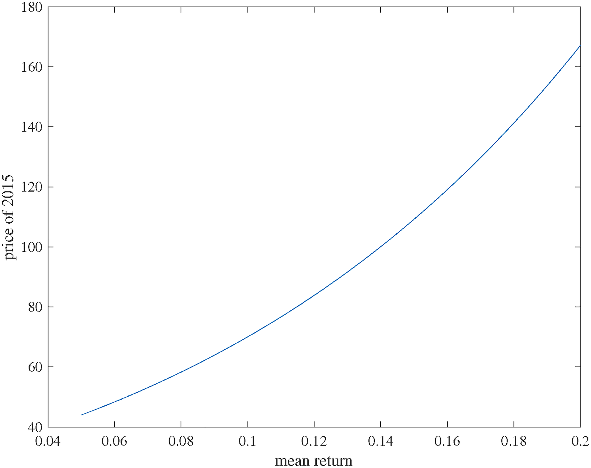
Prices for 2015 at different returns, using the carbon price for 2005 calculated by nordhaus¹² as the initial value.

Table 1.

The price movement process of carbon allowances as an asset versus the optimal carbon price.

	2005($)	2015
Nordhaus¹²	27	42
0.05	27	43.98
0.1	27	70.03
0.15	27	109.23
0.2	27	167.18

[1] The first row of the table shows the optimal carbon price for different periods in Nordhaus,¹² while the following rows show the price of carbon allowances as a tradable asset for different periods at different rates of return.

[2] Source: Golosov et al..⁹

Next, we will compare the results of the optimal carbon tax calculated by the well-known Stern and Stern¹³ method and carbon allowance price movements.

According to Table 2 and Figure 6, at a return of 0.05, the price of carbon allowances in 2020 and 2025 looks comparable to the optimal tax. However, when we put the timeline a little longer. Near 2050, the price of continuously storable traded carbon allowances will rise to near $1,000, which would be significantly more than a reasonable carbon tax. Not to mention higher yields. If we consider the realistically observed yield of around 0.2, the price of carbon allowances will rise to the unattainable figure of $100,000, ignoring of course, the possible complete substitution of clean energy for fossil fuels.

Figure 6.

Prices for 2025 at different returns, using the carbon price for 2015 calculated by nordhaus⁸ of stern and stern¹³ as the initial value.

Table 2.

The price movement process of carbon allowances as an asset versus the optimal carbon price.

	2015($)	2020	2025	2030	2050
Stern and Stern¹³	197.4	266.5	324.6	376.2	629.2
0.05	197.4	251.94	321.54	410.38	1088.86
0.1	197.4	317.91	512.00	824.59	5547.42
0.15	197.4	397.04	798.59	1606.26	26288.85
0.2	197.4	491.19	1222.25	3041.35	116597.91

[1] The first row of the table shows the optimal carbon price for different periods in Stern and Stern¹³ and computed in Nordhaus,⁸ while the following rows show the price of carbon allowances as a tradable asset for different periods at different rates of return.

[2] Source: Nordhaus.⁸

Compared to Stern and Stern,¹³ Nordhaus⁸ offers a more moderate level of carbon taxation. This also implies that the price movement of carbon allowances is more different from the optimal carbon tax calculated by Nordhaus.⁸ According to Table 3 and Figure 7, even at a return level of 0.05, the price of carbon allowances in 2050 exceeds the optimal carbon tax by about 70%. And at a return level of 0.2, the price of carbon allowances in 2050 would be 18 times higher than the optimal carbon tax.

Figure 7.

Prices for 2025 at different returns, using the carbon price for 2015 calculated by nordhaus⁸ as the initial value.

Table 3.

The price movement process of carbon allowances as an asset versus the optimal carbon price.

	2015($)	2020	2025	2030	2050
Nordhaus⁸	31.2	37.3	44	51.6	102.5
0.05	31.2	39.82	50.82	64.86	172.10
0.1	31.2	50.25	80.92	130.33	876.80
0.15	31.2	62.75	126.22	253.88	4155.08
0.2	31.2	77.64	193.18	480.70	18428.85

[1] The first row of the table shows the optimal carbon price for different periods in Nordhaus,⁸ while the following rows show the price of carbon allowances as a tradable asset for different periods at different rates of return.

[2] Source: Nordhaus.⁸

Results and discussion

One of the central issues in environmental economics has been how to solve environmental-related problems with externalities. Quantitative and price approaches are currently the main candidates for solving this problem.

The theoretical origin of the use of the price approach, i.e. the taxation of emissions, comes from the idea of Pigou's taxation of excess net benefits.¹⁴ If policymakers can accurately measure the externalities generated by emissions, then a direct tax on the environment would reconcile the Decentralized Equilibrium with the results of the Planning Problem. However, the difficulty with this solution is that it is difficult to measure the externalities from emissions precisely and, therefore, to measure the most tax accurately.

In contrast, the quantitative approach quantifies emissions as a right, with the government issuing a set number of allowances that symbolise the right to emit and requiring companies to pay the number of allowances that correspond to their emissions. The quantitative approach has its theoretical roots in Coase's rethinking of the Pigouvian taxation scheme, seeing.²⁷ At the governmental level, the quantitative approach avoids the problem of estimating the tax and instead only requires the consideration of emission limits. At the same time, if the government uses paid distribution methods such as auctions, the government also receives the corresponding revenue, so the quantitative approach can also have the double dividend of a taxation scheme.

However, Coase's theorem does not guarantee that the economy will develop dynamically in the optimal path shown in the Planning Problem, and it is from this perspective that this paper explores whether the economy will spontaneously run on an optimal path if the quantitative approach is used.

In our results, we find that the quantity approach does impose an additional cost on the emitting firm in the Decentralized Equilibrium, but this cost is not necessarily equal to the externality. Indeed, as the supply of allowances is determined by the investors who hold them, the movement of the price of allowances is determined by the pricing kernel rather than the externality it generates. Therefore, the movement of the price of carbon allowances does not match the movement of the carbon externality corresponding to the path of the social planner.

This result has strong policy implications. Both China and the EU allow manufacturers to save carbon allowances for the next period or even to pre-borrow them from the next period, a policy that is in essence consistent with the setting in the Decentralised Equilibrium. In both the Chinese and EU carbon markets, investors in carbon allowances have become an important factor in the price movement of carbon allowances. The price movement process of carbon allowances relies on pricing kernels rather than externalities. However, in the case of the Planning Problem, the corresponding carbon price should come from the magnitude of the externality. The difference between the carbon price in the Chinese and EU markets and the path of the carbon price in the Planning Problem could lead to the economy not growing in an optimal path.

Our results do not imply a complete failure of carbon allowance policies. In fact, in our literature review, we have described previous studies in which carbon allowance policies used only in the current period can keep the economy on an optimal path. On the other hand, a reasonable carbon tax can also keep the economy on an optimal path. However, as pointed out by Coase,²⁷ quantifying the price of carbon in each period is a very difficult task, so a carbon tax becomes difficult to implement. On the other hand, it has always been relatively easy for policymakers to measure the total carbon emissions cap over an infinite number of periods, but our study demonstrates that policymakers also need to plan for carbon emissions in each period. Unfortunately, our study brings bad news for policymaking, as policymakers need to put in more effort to plan for more detailed carbon emissions. In terms of the carbon tax measurement process, the difficulty of planning each year's carbon emissions is comparable to the difficulty of developing a dynamic carbon tax. Policymakers can therefore return to the starting point of the two policy divergences, i.e. the choice to suffer from emissions uncertainty or carbon price uncertainty.

In the particular steady-state, we find that consumption in the steady-state is found to be determined by the rate of technological progress, the total amount of carbon dioxide at steady-state, the level of technology at which steady-state is reached and the total amount of carbon allowances remaining. It is worth mentioning that there is a limit to the growth of steady-state consumption with respect to the rate of technological progress. This is because our model assumes that economic development is constrained by fossil energy. Even if the rate of technological progress is very fast, the consumption in the first period after reaching the steady-state is the output obtained by consuming almost all fossil energy at the current level of technology. On the other hand, the effect of total carbon dioxide at steady-state on steady-state consumption is almost linear.

As an application of the theory, we compare the movement of the price of carbon allowances with the difference between Nordhaus,¹² Stern and Stern¹³ and Nordhaus.⁸ We find that in the short run, the price movement of carbon allowances is close to the optimal carbon tax if the average return on carbon allowances is around 5% (the average return in EU Phase III is around 20%). In the long run, on the other hand, any average return of 5% and above causes the price of carbon allowances to increase much faster than the optimal carbon tax. This means that trading carbon allowances across time will allow economies to consume too much fossil fuel in the early years.

Conclusions

Our model demonstrates that if carbon allowances in the carbon market are free to be used in each period, the path of economic growth and the optimal path are different. This implies that the carbon allowance policies used in the EU and China are ineffective in terms of the path of economic development. If policymakers wish to continue to use carbon allowances as an environmental policy to control carbon emissions, they should set the carbon emissions for each period. At the same time, research in the steady-state leads us to find that increasing the rate of technological progress is a proven option for increasing total social welfare.

Details of the planning problem

We use the bellman function method to solve this problem:

V (K_{t}, S_{1, t}, S_{2, t}, R_{t}, z_{t}) = \max_{{C_{t}, K_{t + 1}, K_{1, t}, K_{2, t}, L_{t}, L_{1, t}, L_{2, t}, E_{t}, R_{t + 1}, S_{1, t + 1}, S_{2, t + 1}}}

U (C_{t}, 1 - L_{t}) + β E_{t} V (K_{t + 1}, S_{1, t + 1}, S_{2, t + 1}, R_{t + 1}, z_{t + 1})

(80)

s . t . C_{t} + K_{t + 1} = F_{1} (K_{1, t}, L_{1, t}, E_{t}, R_{t}, z_{t}) + K_{t},

(81)

K_{1, t} + K_{2, t} = K_{t},

(82)

E_{t} = F_{2} (K_{2, t}, L_{2, t}, S_{1, t} + S_{2, t}, z_{t}),

(83)

L_{1, t} + L_{2, t} = L_{t},

(84)

S_{1, t + 1} = (1 - ϕ) S_{1, t} + a E_{t},

(85)

S_{2, t + 1} = S_{2, t} + b E_{t} - H_{t},

(86)

R_{t + 1} = R_{t} - E_{t},

(87)

z_{t + 1} = F_{z} (z_{t}, ϵ_{t}) .

(88)

This can be further written as:

V (K_{t}, S_{1, t}, S_{2, t}, R_{t}, z_{t}) = \max_{{C_{t}, K_{t + 1}, K_{1, t}, K_{2, t}, L_{t}, L_{1, t}, L_{2, t}, E_{t}, λ_{1, t}, λ_{2, t}, λ_{3, t}, λ_{4, t}, λ_{5, t}, λ_{6, t}, λ_{7, t}, λ_{8, t}, R_{t + 1}, S_{1, t + 1}, S_{2, t + 1}}}

U (C_{t}, 1 - L_{t}) + β E_{t} V (K_{t + 1}, S_{1, t + 1}, S_{2, t + 1}, R_{t + 1}, z_{t + 1})

+ λ_{1, t} (F_{1} (K_{1, t}, L_{1, t}, E_{t}, S_{1, t} + S_{2, t}, z_{t}) + K_{t} - C_{t} - K_{t + 1})

+ λ_{2, t} (K_{t} - K_{1, t} - K_{2, t})

+ λ_{3, t} (F_{2} (K_{2, t}, L_{2, t}, R_{t}, z_{t}) - E_{t})

+ λ_{4, t} (L_{t} - L_{1, t} - L_{2, t})

+ λ_{5, t} ((1 - ϕ) S_{1, t} + a E_{t} - S_{1, t + 1})

+ λ_{6, t} (S_{2, t} + b E_{t} - H_{t} - S_{2, t + 1})

+ λ_{7, t} (R_{t} - E_{t} - R_{t + 1})

+ λ_{8, t} (F_{z} (z_{t}, ϵ_{t}) - z_{t + 1}) .

(89)

The first-order condition are (

z_{t}

is not to be considered for exogenous processes):

U_{C_{t}} = λ_{1, t},

(90)

U_{L_{t}} = - λ_{4, t},

(91)

λ_{1, t} F_{1 K_{1, t}} - λ_{2, t} = 0,

(92)

λ_{3, t} F_{2 K_{2, t}} - λ_{2, t} = 0,

(93)

λ_{1, t} F_{1 L_{1, t}} - λ_{4, t} = 0,

(94)

λ_{3, t} F_{2 L_{2, t}} - λ_{4, t} = 0,

(95)

λ_{1, t} F_{1 E_{t}} - λ_{3, t} + λ_{5, t} a + λ_{6, t} b - λ_{7, t} = 0,

(96)

β E_{t} V_{K_{t + 1}} = λ_{1, t},

(97)

β E_{t} V_{S_{1, t + 1}} = λ_{5, t},

(98)

β E_{t} V_{S_{2, t + 1}} = λ_{6, t},

(99)

β E_{t} V_{R_{t + 1}} = λ_{7, t},

(100)

C_{t} + K_{t + 1} = F_{1} (K_{1, t}, L_{1, t}, E_{t}, S_{t}, z_{t}) + K_{t},

(101)

K_{1, t} + K_{2, t} = K_{t},

(102)

E_{t} = F_{2} (K_{2, t}, L_{2, t}, S_{t}, z_{t}),

(103)

L_{1, t} + L_{2, t} = L_{t},

(104)

S_{1, t + 1} = (1 - ϕ) S_{1, t} + a E_{t},

(105)

S_{2, t + 1} = S_{2, t} + b E_{t} - H_{t},

(106)

R_{t + 1} = R_{t} - E_{t} .

(107)

The envelope theorem yields

V_{K_{t}} = λ_{1, t} + λ_{2, t},

(108)

V_{S_{1, t}} = λ_{2, t} F_{1 S_{1, t}} + (1 - ϕ) λ_{5, t},

(109)

V_{S_{2, t}} = λ_{2, t} F_{1 S_{2, t}} + λ_{6, t},

(110)

V_{R_{t}} = λ_{3, t} F_{2 R_{t}} + λ_{7, t} .

(111)

Combined (90), (91) and (94), we have :

U_{C_{t}} F_{1 L_{1, t}} + U_{L_{t}} = 0.

(112)

This equation represents the first-order conditions for consumer decisions. Combined (90), (91), (92), (93) and (95), we have :

\frac{U_{C_{t}} F_{1 K_{1, t}} F_{1 L_{2, t}}}{F_{2 K_{2, t}}} + U_{L_{t}} = 0.

(113)

Combined (90), (92), (97) and (108), we have :

β E_{t} (U_{C_{t + 1}} + U_{C_{t + 1}} F_{1 K_{1, t + 1}}) = U_{C_{t}} .

(114)

Though (90), (92), (93), (98) and (109), it can be deduced that :

β E_{t} (U_{C_{t + 1}} F_{1 K_{1, t + 1}} F_{1 S_{1, t + 1}} + (1 - ϕ) λ_{5, t + 1}) = λ_{5, t} .

(115)

Combined (90), (92), (93), (99) and (110), we have :

β E_{t} (U_{C_{t + 1}} F_{1 K_{1, t + 1}} F_{1 S_{2, t + 1}} + λ_{6, t + 1}) = λ_{6, t} .

(116)

With (100) and (111), we deduce that:

β E_{t} (\frac{U_{C_{t} + 1} F_{1 K_{1, t + 1}}}{F_{2 K_{2, t + 1}}} F_{2 R_{2, t + 1}} + λ_{7, t + 1}) = λ_{7, t} .

(117)

Combined (90), (92), (93) and (96), we have :

U_{C_{t}} F_{1 E_{t}} - \frac{U_{C_{t}} F_{1 K_{1, t}}}{F_{2 K_{2, t}}} + λ_{5, t} a + λ_{6, t} b - λ_{7, t} = 0.

(118)

The Planning Problem is composed of (101), (102), (103), (104), (105), (106), (107), (112), (113), (114), (115), (116), (117) and (118) consisting of fourteen dynamic equations.

Details of the decentralized equilibrium

We use the Bellman equation for the solution ( $η$ is a Lagrange multiplier):

\hat{V} (K_{t}, A_{t}) = \max_{{C_{t}, K_{t + 1}, L_{t}, {\hat{E}}_{t}, A_{t + 1}}} U (C_{t}, 1 - L_{t}) + β E_{t} \hat{V} (K_{t + 1}, A_{t + 1})

(119)

s . t . C_{t} + K_{t + 1} = n_{t} L_{t} + p_{t} {\hat{E}}_{t} + (1 + r_{t}) K_{t},

(120)

A_{t + 1} = A_{t} - {\hat{E}}_{t} .

(121)

The transformation of the maximisation problem using the Lagrangian method yields:

\hat{V} (K_{t}, A_{t}) = \max_{{C_{t}, K_{t + 1}, L_{t}, {\hat{E}}_{t}, A_{t + 1}, η_{1, t}, η_{2, t}}} U (C_{t}, 1 - L_{t}) + β E_{t} \hat{V} (K_{t + 1}, A_{t + 1})

(122)

+ η_{1, t} (n_{t} L_{t} + p_{t} {\hat{E}}_{t} + (1 + r_{t}) K_{t} - C_{t} - K_{t + 1}),

(123)

+ η_{2, t} (A_{t} - {\hat{E}}_{t} - A_{t + 1}) .

(124)

The first-order conditions are

U_{C_{t}} = η_{1, t},

(125)

U_{L_{t}} = - n_{t} η_{1, t},

(126)

p_{t} η_{1, t} = η_{2, t},

(127)

β E_{t} {\hat{V}}_{K_{t + 1}} = η_{1, t},

(128)

β E_{t} {\hat{V}}_{A_{t + 1}} = η_{2, t},

(129)

C_{t} + K_{t + 1} = n_{t} L_{t} + p_{t} {\hat{E}}_{t} + (1 + r_{t}) K_{t},

(130)

A_{t + 1} = A_{t} - {\hat{E}}_{t} .

(131)

Using the envelope theorem it follows that:

{\hat{V}}_{K_{t}} = (1 + r_{t}) η_{1, t},

(132)

{\hat{V}}_{A_{t}} = η_{2, t} .

(133)

Combined (125) and (126), we have :

U_{C_{t}} n_{t} + U_{L_{t}} = 0.

(134)

With (125), (128) and (132), it can be seen that

β E_{t} ((1 + r_{t + 1}) U_{C_{t + 1}}) = U_{C_{t}} .

(135)

Combining (125), (127), (129) and (133), we get

β E_{t} (p_{t + 1} U_{C_{t + 1}}) = p_{t} U_{C_{t}} .

(136)

Consumer choice consists of five dynamic equations (130), (131), (134), (135) and (136).

Footnotes

Declaration of conflicting interests

The author(s) declared no potential conflicts of interest with respect to the research, authorship, and/or publication of this article.

Funding

The author(s) received no financial support for the research, authorship, and/or publication of this article.

ORCID iD

Yu Yan

Notes

Yu Yan PhD candidate in Finance.

Yiming Lei MS in Managerial Economics.

YuYang Tang PhD Candidate in Population, Resources and Environmental Economics.

Xufeng Zhao PhD candidate in Finance.

References

Gardner

Herr

Ostrom

, et al. The power and limitations of proportional cutbacks in common-pool resources. J Dev Econ 2000; 62: 515–533.

Böhringer

Lange

. On the design of optimal grandfathering schemes for emission allowances. Eur Econ Rev 2005; 49: 2041–2055.

Taschini

. Flexibility premium of emissions permits. Journal of Economic Dynamics and Control 2021; 126: 104013.

Tybout

. Pricing pollution and other negative externalities. The Bell Journal of Economics and Management Science 1972; 3: 252–266.

Frech

III . Pricing of pollution: the coase theorem in the long run. The Bell Journal of Economics and Management Science 1973; 4: 316–319.

Jouvet

Michel

Rotillon

. Optimal growth with pollution: how to use pollution permits? Journal of Economic Dynamics and Control 2005; 29: 1597–1609.

Nordhaus

. A review of the stern review on the economics of climate change. J Econ Lit 2007a; 45: 686–702.

Nordhaus

. Revisiting the social cost of carbon. Proc Natl Acad Sci U S A 2017; 114: 1518–1523.

Golosov

Hassler

Krusell

, et al. Optimal taxes on fossil fuel in general equilibrium. Econometrica 2014; 82: 41–88.

10.

Bredin

Parsons

. Why is spot carbon so cheap and future carbon so dear? The term structure of carbon prices. The Energy Journal 2016; 37: 3.

11.

Grübler

Fujii

. Inter-generational and spatial equity issues of carbon accounts. Energy 1991; 16: 1397–1416.

12.

Nordhaus

. To tax or not to tax: alternative approaches to slowing global warming. Review of Environmental Economics and Policy 2007b; 1: 26–44.

13.

Stern

. The economics of climate change: the Stern review. New York: Cambridge University press, 2007.

14.

Pigou

. The economics of welfare. Cambridge: Palgrave Macmillan, 2013.

15.

Griffin

Steele

. Energy economics and policy. London: Elsevier, 2013.

16.

Dolbear

. On the theory of optimum externality. Am Econ Rev 1967; 57: 90–103.

17.

Uzawa

. Economic theory and global warming. New York: Cambridge University Press, 2003.

18.

Goulder

Mathai

. Optimal CO2 abatement in the presence of induced technological change. New York: Routledge, 2010.

19.

Hoel

. Climate change and carbon tax expectations. 2010.

20.

Brännlund

Nordström

. Carbon tax simulations using a household demand model. Eur Econ Rev 2004; 48: 211–233.

21.

Benchekroun

Chaudhuri

. Environmental policy and stable collusion: the case of a dynamic polluting oligopoly. Journal of Economic Dynamics and Control 2011; 35: 479–490.

22.

King

Tarbush

Teytelboym

. Targeted carbon tax reforms. Eur Econ Rev 2019; 119: 526–547.

23.

Ulph

. The optimal time path of a carbon tax. Oxf Econ Pap 1994; 46: 857–868.

24.

Dasgupta

Heal

. Economic theory and exhaustible resources. New York: Cambridge University Press, 1979.

25.

Goulder

. Effects of carbon taxes in an economy with prior tax distortions: an intertemporal general equilibrium analysis. J Environ Econ Manage 1995; 29: 271–297.

26.

Barrage

. Optimal dynamic carbon taxes in a climate– economy model with distortionary fiscal policy. Rev Econ Stud 2020; 87: 1–39.

27.

Coase

. The problem of social cost In: Classic papers in natural resource economics. London: Springer, 1960, pp. 87–137.

28.

Dales

. Pollution, property & prices: an essay in policy- making and economics. Cheltenham: Edward Elgar Publishing, 2002.

29.

Bovenberg

Goulder

. Optimal environ- mental taxation in the presence of other taxes: general- equilibrium analyses. Am Econ Rev 1996; 86: 985–1000.

30.

Elkins

Baker

. Carbon taxes and carbon emissions trading. J Econ Surv 2001; 15: 325–376.

31.

Goulder

Parry

Burtraw

. Revenue- raising vs. Other approaches to environmental protection: the critical significance of pre-existing tax distortions. Technical Report, National Bureau of Economic Research 1996.

32.

Parry

. Fiscal interactions and the case for carbon taxes over grandfathered carbon permits. Oxford Review of Economic Policy 2003; 19: 385–399.

33.

Mathys

de Melo

. Political Economy Aspects of Climate Change Mitigation Efforts. World Economy 2011; 34(11): 1938–1954.

34.

Weitzman

. Prices vs. Quantities. Rev Econ Stud 1974; 41: 477–491.

35.

Parker

. Carbon tax and greenhouse gas control: options and considerations for congress. Library of Congress. Congressional Research Service. 2009.

36.

Zakeri

Dehghanian

Fahimnia

, et al. Carbon pricing versus emissions trading: a supply chain planning perspective. Int J Prod Econ 2015; 164: 197–205.

37.

Hope

. Discount rates, equity weights and the social cost of carbon. Energy Economics 2008; 30: 1011–1019.

38.

Zhang

Wang

Tan

. The impact of China’s carbon allowance allocation rules on the product prices and emission reduction behaviors of ets-covered enterprises. Energy Policy 2015; 86: 176–185.

39.

Geng

Dai

, et al. A general equilibrium analysis on the impacts of regional and sectoral emission allowance allocation at carbon trading market. J Cleaner Prod 2018; 192: 421–432.

40.

Forbes

Zampelli

. Wind energy, the price of carbon allowances, and CO₂ emissions: evidence from Ireland. Energy Policy 2019; 133: 110871.