Quantitative palaeoclimate reconstruction as an inverse problem: A Bayesian inference of late-Holocene climate on the eastern Tibetan Plateau from a peat cellulose δ 18 O record

Abstract

There has been a sustained need to quantify past climate changes from proxy records to better understand the driving mechanisms and thus to improve the prediction of the future. Transfer function is an intuitive and frequently used method in this regard. However, this method is unable to provide interpretive and predictive results from proxy records, because physical processes are not included. The inverse proxy modelling method opened up a new avenue for quantitative palaeoclimate reconstructions through the integration of proxy records with deterministic models. It is fundamentally different from the statistical approach, representing a conceptual advance in quantitative palaeoclimatology. Here we demonstrate the potential of this method by placing a mechanistic model and a 6000 year long peat cellulose δ¹⁸O record obtained from the high-cold and monsoonal eastern Tibetan Plateau (c. 3500 m a.s.l.) in a Bayesian paradigm. In this worked example, the marginal posterior probability distributions of palaeoclimate variables such as the δ¹⁸O of soil water, temperature, and relative humidity were inferred jointly through the solution to an ill-posed inverse problem using the Markov chain-Monte Carlo method. Our results indicate that the observed variation of the peat cellulose δ¹⁸O record in this monsoonal area essentially reflects the changes in the oxygen isotopic composition of soil water, which is closely linked to that of rainfall. Compared with hydrology, temperature and humidity have little influence on the oxygen isotope fractionation of leaf water.

Keywords

Bayesian inference inverse proxy modeling Markov chain Monte Carlo quantitative palaeoclimate reconstruction transfer function

Introduction

Quantitative palaeoclimate information obtained from various proxies may not only deepen our insight into the mechanisms of past climate changes, but also constitute a primary knowledge base for predicting the future. A commonly followed approach to quantifying past climate changes from proxy records is the transfer function method (Birks, 1995; Bryson and Kutzbach, 1974; Huntley and Prentice, 1988; Imbrie and Kipp, 1971). The essence of this method is first to establish an empirical relationship between proxy data and climate variables based on modern observations, and then use this to translate fossil proxy records to quantitative palaeoclimate data. However, as criticized by Guiot et al. (2000), this method has several inherent drawbacks. First, the empirical relationship established under modern boundary conditions may not hold for the past. The best example in this regard is the pollen–climate transfer function. All these kinds of regression equations do not take into account the time-varying atmospheric CO₂ level, which is a crucial limiting factor for vegetation growth (Cowling and Sykes, 1999). Second, the reference modern proxy data used to constrain the transfer function may have been disturbed by human activity, leading to a biased statistical relationship that is inapplicable to render the proxy records in climatic terms. The final caveat is that the statistical relationship based on spatially distributed modern data may be incomplete because of lack of adequate analogs for the past (Jackson and Williams, 2004).

Many attempts have been made to overcome the aforementioned limitations (Bhattacharya, 2006; Guiot, 1990; Haslett et al., 2006; Korhola et al., 2002; Kühl et al., 2002; Mosbrugger and Utescher, 1997; Robertson et al., 1999; Toivonen et al., 2001; Vasko et al., 2000; Wolfe, 1995). However, none of these methods considers the underlying physical processes that control the formation of the proxies, and thus still unable to yield interpretive results of the proxies. Assimilations of proxy data in process-based deterministic models have shown great potential in palaeoclimatological studies (Gebbie and Huybers, 2006; Gebka et al., 1999; Hargreaves and Annan, 2002; Heinze and Hasselmann, 1993; Hopcroft et al., 2009; Huybers et al., 2007; LeGrand and Wunsch, 1995; McKeague et al., 2005; Rajver et al., 1998; Widmann et al., 2010; Wunsch, 2003). This concept was first introduced to the area of quantitative palaeoclimatology by Guiot et al. (2000), who also gave it the name ‘Inverse Proxy Modeling’ (Guiot et al., 2009). Although this method has been extensively used to quantify past climate changes from pollen records in conjunction with mechanistic vegetation models within the framework of Bayesian statistical inference over the past decade (Garreta et al., 2010; Guiot et al., 2000; Hatté and Guiot, 2005; Hatté et al., 2009; Rousseau et al., 2006; Wu et al., 2007a, b), its utility for inversion of past climate from other abiotic proxy records has never been tested. Here we conduct a Bayesian inversion of climate changes on the eastern Tibetan Plateau during the last 6000 years through integrating a peat cellulose δ¹⁸O record with a simplistic yet mechanistic model of oxygen isotope fractionation in plant cellulose. Our results show that this proxy data-model fusion technique is a promising way to quantify the climate information of the past mechanistically.

Basic concepts and theoretical framework of the inverse proxy modeling method

In this section, we explain the philosophy of the inverse proxy modeling method. Instead of presenting a comprehensive discussion, here we only introduce the main elements and outline the general theoretical framework. For a full account of this method, readers are referred to Guiot et al. (2009). The conceptual difference between the transfer function and the inverse proxy modeling methods is illustrated in Figure 1. The transfer function method intuitively expresses climate variables as a function of proxy data using empirical constraints through regression analyses (Figure 1A):

climate = f (proxy data)

(1)

Figure 1.

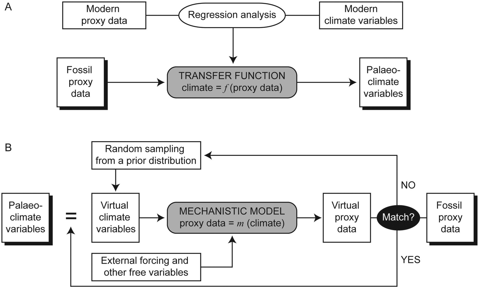
Diagrams illustrating the difference in concept between the traditional transfer function method (A) and the inverse proxy modeling method (B)

Conversely, the inverse proxy modeling method treats climate variable as the parameters of mechanistic models that describe the formation of proxy data (Figure 1B):

proxy data = m (climate)

(2)

Specifically, if the physics behind the climate proxies is known, then we can put forward a deterministic model, say m(θ), with parameters θ being some major climate variables. Unlike the forward modeling, which is aimed at providing mechanistic interpretations of the proxy data, the inverse modeling is to find an optimal estimate of model parameters from proxy data. Through solving this problem, quantitative palaeoclimate information may be obtained.

The inverse proxy modeling method yields quantitative palaeoclimate information not as straightforward as the transfer function method does. It first randomly generates a candidate set of the climate variables, which is then input to the mechanistic models along with other forcing factors and complementary environmental variables to generate a simulated proxy record that is to be compared with the fossil proxy record (Figure 1B). If both data sets match to some degree, keep this candidate; otherwise, reject and repeat the above procedure until acceptable values are obtained. Perturb these values iteratively in their parameter space and repeat the whole procedure for a thousand times or even more to build frequency histograms, which mimic the probability distributions of the palaeoclimate variables.

In practice, the key issue is how to define and evaluate the matching. Techniques diverge at this step. The least-squares inversion method minimizes the sum of squares of the model residuals to solve for parameters θ:

\overset{⌢}{θ} = \arg \min_{θ} {‖ y - m (θ) ‖}^{2}

(3)

where y is the proxy record, θ the climate variables, m(θ) the modeled proxy record, and $\hat{θ}$ the optimal estimate for θ. This method may be less robust or may even fail to work, if a small number of outliers exit in the observational data (Tarantola, 2005). Alternatively, if the model residual is regarded as a continuous random variable with probability density function p(y|m(θ)), the matching could be defined as a likelihood function:

ℓ (y | m (θ)) = \prod_{i}^{N} p (y_{i} | m_{i} (θ))

(4)

where N is the length of the observational data set. An optimal estimate for parameters θ may be obtained by maximizing this likelihood function. Because the inverse problem usually is ill-posed, particularly when the model is nonlinear, the solution may not exist in the strict sense or may not be unique (Blaauw et al., 2010).

Bayesian inference appears to be a powerful and increasingly popular method for solving complex inverse problems in a conceptually simple and theoretically unified way (Gilks et al., 1996). It is a probabilistic approach in which all sorts of uncertainty are expressed in terms of probability density functions. The implementation generally consists of three steps. First, we need to formulate a statistical model (i.e. the likelihood function) that could adequately describe the relationship between our beliefs about m(θ) and the proxy record y. Then we propose an initial belief (i.e. the prior probability) about parameters θ. Finally, we apply Bayes’ rule to obtain an updated belief (i.e. the posterior probability) of these parameters:

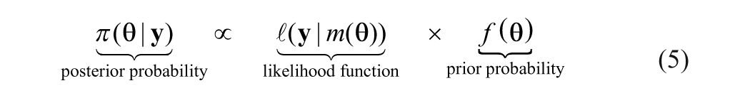
\underset{posterior probability}{\underset{︸}{π (θ | y)}} \propto \underset{likelihood function}{\underset{︸}{ℓ (y | m (θ))}} \times \underset{prior probability}{\underset{︸}{f (θ)}}

(5)

The posterior probability distribution usually cannot be given analytically because of its mathematical complexity, but it can be simulated using the Markov chain-Monte Carlo (MCMC) method. From such a probabilistic expression, we can easily calculate some statistical moments such as the mean, median, and variance of parameters θ so as to address the uncertainty of the solution.

Model, data, and algorithm

It has long been known that the enrichment of the heavy oxygen isotope in plant vascular tissue reflects the average growing conditions of the plant as a function of temperature, humidity, and water availability (Burk and Stuiver, 1981; Epstein and Yapp, 1977; Gray and Thompson, 1976). Therefore, measuring the oxygen isotopic composition of plant remains such as tree-ring (Raffalli-Delerce et al., 2004) and peat cellulose (Helliker and Ehleringer, 2002) may reveal past climate conditions. However, most of these attempts were made in a qualitative way (Brenninkmeijer et al., 1982; Hong B.et al., 2009; Hong Y.T. et al., 2000; Ménot-Combes et al., 2002; Xu et al., 2006). In this section, we provide an example to illustrate how quantitative palaeoclimate information can be retrieved by assimilating a peat cellulose δ¹⁸O record in a simplistic yet mechanistic model of oxygen isotope fractionation in plant cellulose using Bayesian inference.

Model of oxygen isotope fractionation in plant cellulose

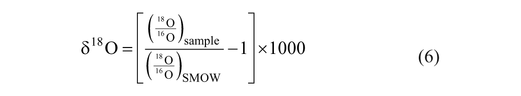
The model of oxygen isotope fractionation in plant cellulose was established by Roden et al. (2000). It is composed of two major components: one describes the biophysical processes that lead to the enrichment of the heavy oxygen isotope in leaf water, and the other accounts for the biochemical processes governing the oxygen isotope exchange between different organic components during cellulose synthesis. In this model, the oxygen isotope ratio is normalized to the standard mean ocean water (SMOW) in parts per thousand using the delta notation:

δ {}^{18}O = [\frac{{(\frac{{}^{18}O}{{}^{18}O})}_{sample}}{{(\frac{{}^{18}O}{{}^{18}O})}_{SMOW}} - 1] \times 1000

The essential biophysical process linking the oxygen isotopic composition of leaf water with climate is evapotranspiration, which leads to a progressive enrichment of the heavy oxygen isotope in leaf water with respective to that in soil water. This process was first modeled by Dongmann et al. (1974) based on the equation for oxygen isotope fractionation in an open water body during the phase change from liquid to vapor and during molecular diffusion (Craig and Gordon, 1965). The oxygen isotopic composition of leaf water can be expressed as:

δ^{18} O_{1} = δ^{18} O_{s} + ε_{eq} + ε_{k} + (δ^{18} O_{a} - δ^{18} O_{s} - ε_{k}) \times h

(7)

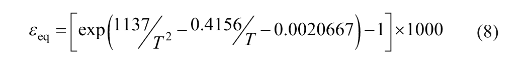
where subscripts l, s and a refer to leaf water, soil water, and the atmospheric water vapor, respectively, h is the relative humidity, ε_k the kinetic separation parameter, which is set to 16‰ according to the relative rate of molecular diffusion of ¹⁶O and ¹⁸O in the turbulent boundary layer (Dongmann et al., 1974), and ε_eq the equilibrium separation parameter, which can be expressed as a function of absolute temperature (T) in degrees Kelvin (Majoube, 1971):

ε_{eq} = [\exp (\frac{1137}{T^{2}} - \frac{0.4156}{T} - 0.0020667) - 1] \times 1000

(8)

Assuming that the meteoric water is predominantly from the well-mixed regional air mass that is in equilibrium with soil water, the δ¹⁸O shift of atmospheric water vapor relative to soil water, denoted by δ¹⁸O_a−δ¹⁸Os, is governed by the equilibrium fractionation, i.e. δ¹⁸O_a−δ¹⁸Os = −ε_eq. Therefore, Eq. (7) can be further simplified as:

δ^{18} O_{1} = δ^{18} O_{s} + (ε_{eq} + ε_{k}) \times (1 - h)

(9)

The photosynthesis generally can increase the δ¹⁸O value by about 27‰ in leaf cellulose during the interaction between carbonyl and soil water (Yakir and DeNiro, 1990). In addition, a secondary fractionation may occur, if there is a partial equilibrium exchange between the synthesized carbohydrate and soil water. Taken together, the isotopic composition of plant cellulose can be expressed as:

δ^{18} O_{c} = f_{o} \times (δ^{18} O_{s} + ε_{o}) + (1 - f_{o}) \times (δ^{18} O_{1} + ε_{o})

(10)

where ϵ_o = 27‰ is a biochemical fractionation factor (Yakir and DeNiro, 1990), and f _o = 0.42 is the proportion of the carbon-bound oxygen undergoing exchange with soil water (Roden et al., 2000).

The δ¹⁸O value of plant cellulose now is reduced to a function of parameter vector θ = [δ¹⁸O_s,T,h], which will be inferred herewith.

Description of the peat cellulose δ¹⁸O record

The δ¹⁸O record of bulk peat α-cellulose is derived from the Hongyuan Peatland (32°46′N, 102°30′E). Situated on the northeastern edge of the Tibetan Plateau (Figure 2A), it is the world’s highest (c. 3500 m a.s.l.) wetland ecosystem dominated by Carex mulieensis. The climate condition in Hongyuan ranges from cool to cold with a sharp seasonal shift, reflecting the influence of the Indian Monsoon (Xu et al., 2006). Mean annual relative humidity is about 0.7, and mean annual precipitation is 650 mm. Modulated by the South Asian monsoon, most of the precipitation occurs in summer months. The interannual variation of both relative humidity and mean annual precipitation is mild, while mean annual temperature shows a remarkable fluctuation, varying between 0.5 and 4.0°C. Given this climate setting, the 6000 year long δ¹⁸O record (Figure 1B), supported by seven AMS radiocarbon ages (Xu et al., 2006), primarily reveals orbital-scale changes in the Indian summer monsoon driven by summer insolation (Berger and Loutre, 1991). Superimposed on this long-term trend are small-scale fluctuations, which have been interpreted as changes in temperatures presumably modulated by variable solar activity (Xu et al., 2006).

Figure 2.

(A) Shaded relief map showing the topographical feature of the Tibetan Plateau. Solid dot indicates the location of the Hongyuan Peatland from where the peat cellulose δ¹⁸O record was derived (Xu et al., 2006). AAM, Arctic air mass; WJS, westerly jet stream; EAM, East Asian monsoon; SAM, South Asian monsoon. (B) Changes in the peat cellulose δ¹⁸O values during the last 6000 years (reversed scale) and comparison with summer insolation at 30°N

The Hasting-within-Gibbs algorithm

The relationship between data and model can be expressed as:

y = δ^{18} O_{c} (θ) + ε

(11)

Here we consider addictive white noise sequence, ε, as independent and identically distributed Gaussian with mean vector µ = 0_L and unknown positive definite covariance matrix Σ = σ²I_L×L, where 0L is a vector made of L zeros, I_L×L an identity matrix with dimension of L×L, and L the length of the data set. Accordingly, the likelihood function is defined as:

ℓ (y | θ, σ^{2}) = {(\frac{1}{2 π σ^{2}})}^{\frac{L}{2}} \exp [- \frac{{‖ y - δ^{18} O_{c} (θ) ‖}^{2}}{2 σ^{2}}]

(12)

With the definition of their prior probability distributions (Appendix 1), a straightforward use of the Bayesian theorem yields the posterior probability distributions of the parameters:

π (θ, σ^{2} | y) \propto ℓ (y | θ, σ^{2}) \times f (θ) \times f (σ^{2}) = {(\frac{1}{2 π σ^{2}})}^{\frac{L}{2} + 1} \exp [- \frac{{‖ y - δ^{18} O_{c} (θ) ‖}^{2}}{2 σ^{2}}] \times f (δ^{18} O_{s}) \times f (T) \times f (h)

(13)

We estimate parameter θ and σ² using the Hasting-within-Gibbs method, which is outlined in Algorithm 1. The MCMC method is used to simulate the marginal posterior probability distribution of parameters T and h. In addition to the Hasting-type move, a scheme of reversible jump is followed to accelerate the mixing of the Markov chains (Appendix 2). If the move of the chains for these two parameters is acceptable, then δ¹⁸O_s and σ² were updated sequentially using a Gibbs sampler (Appendix 3).

Results

The marginal posterior probability distributions of parameter θ and σ² were simulated using Markov chains of 50000 iterations (Figures 3 and 4). Samples were drawn from the chains once they reached a stationary state after the burin-in period (about the first 5000 iterations). To reduce the storage requirement and to remove the autocorrelation of the samples, we thin out the chains by keeping only every tenth values during the run, which are used to calculate the statistical moments such as the mean and standard deviation of parameter θ and to generate frequency histogram of σ² that mimic its posterior probability distribution.

Figure 3.

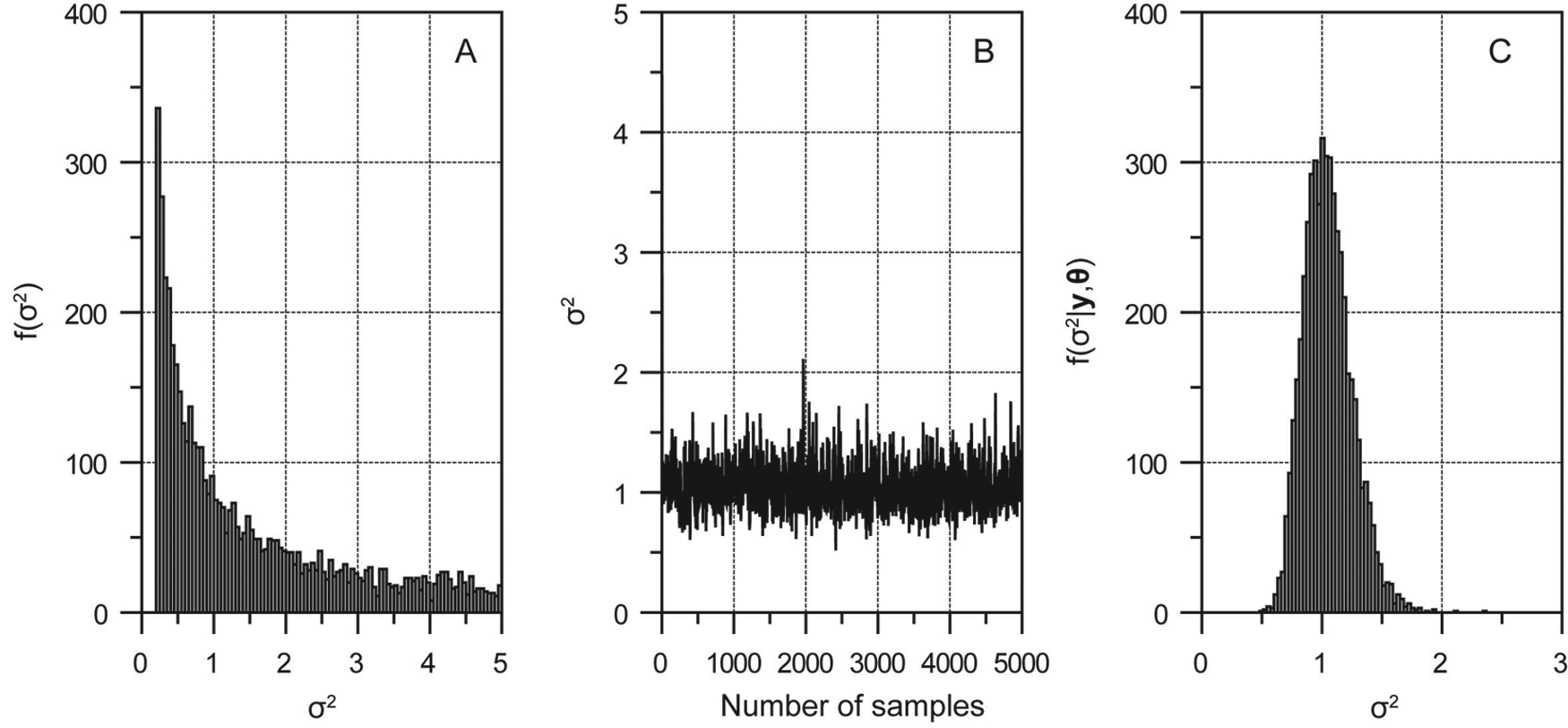
(A) Prior probability distribution of covariance σ², which is assumed to follow a weakly informative Jeffreys’ distribution. (B) Markov chain of σ² thinned out by keeping only every tenth values after the burn-in period. (C) Histogram showing the simulated marginal posterior probability distribution of σ² using the Markov chain

Figure 4.

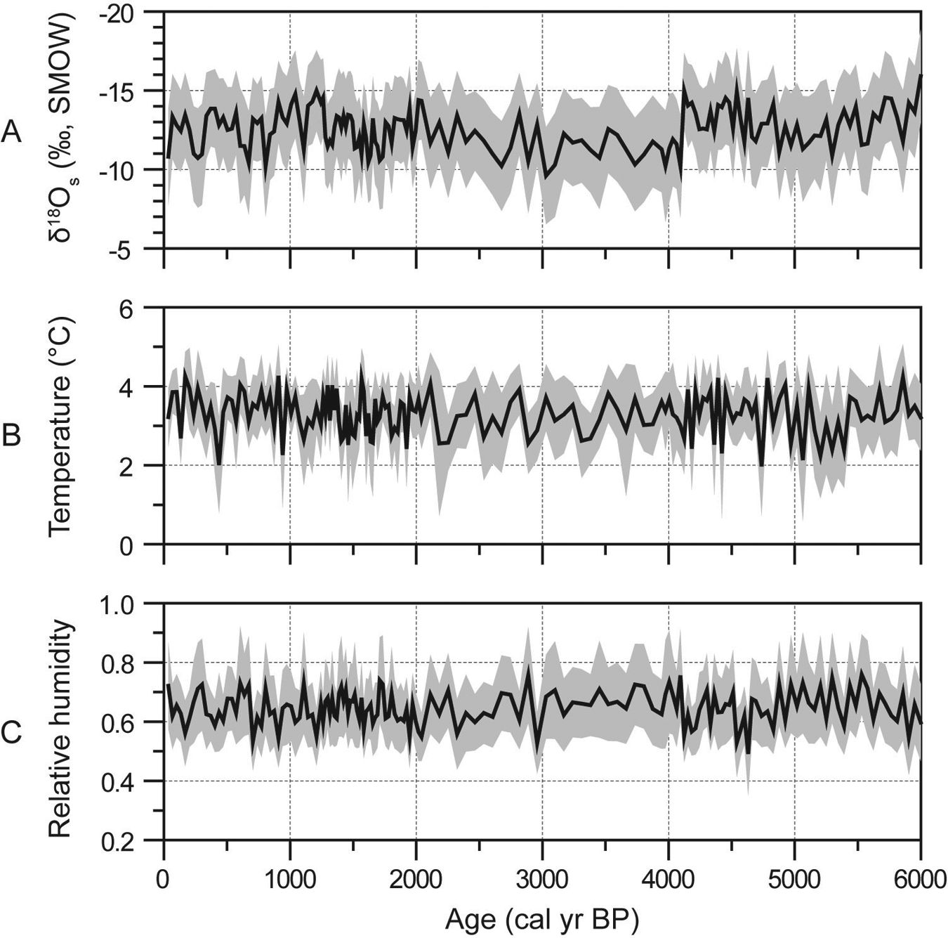
Quantitative palaeoclimate information inferred from the Hongyuan peat cellulose δ¹⁸O record. (A) δ¹⁸O values of soil water. Note vertical axis in reverse order. (B) Annual mean air temperature. (C) Relative humidity. The posterior probability distributions of these variables are summarized using the mean and the standard deviation as denoted by the solid lines and the lightly shaded envelopes, respectively

Figure 3 demonstrates how the prior belief of σ² can be updated using the proxy record and a given likelihood function. A weakly informative Jeffreys’ prior was used to address the non-negativity of σ² (Figure 3A). By taking advantage of the hybrid Metropolis-Hasting-Gibbs algorithm, the Markov chain for σ² converges rapidly (Figure 3B). The frequency histogram of samples drawn from this chain is presented in Figure 3C. As proved in Appendix 3, the marginal posterior probability of σ² follows an inverse Gamma distribution with a mode close to 1 (Figure 3C).

Instead of using a histogram as for σ², the marginal posterior probability distributions of the palaeoclimate variables are visualized using the mean and the standard deviation, which are presented in Figure 4. The δ¹⁸O of soil water exhibits large variability between −15 and −10‰ (Figure 4A), dominating the variance of the peat cellulose δ¹⁸O record. Also, the average value of our reconstructed δ¹⁸O of soil water is very close to that of present-day precipitation, i.e. −12‰ (Zhang et al., 2001), suggesting that the δ¹⁸O of soil water strongly depends on that of precipitation. In contrast, the annual mean temperature shows subtle fluctuations between 2 and 4°C (Figure 4B). The reconstructed relative humidity was stabilized at about 0.6 (Figure 4C), revealing the dominance of monsoonal climate in this area throughout the last 6000 years.

Discussion

The oxygen isotope-based palaeoclimate reconstructions heavily rely on a statistical relationship that links the oxygen isotopic composition of precipitation to temperature (Dansgaard, 1964). This is true at a global scale. However, in the monsoonal areas, the δ¹⁸O of precipitation does not show any correlation with temperature; rather, it is negatively correlated to precipitation known as the ‘amount effect’ (Araguás-Araguás et al., 1998). The climatic conditions in our study area are dominated by the Indian Monsoon. Our reconstructed relative humidity implies that the monsoonal climate might have prevailed during the last 6000 years. Therefore, the large variations in our reconstructed δ¹⁸O of soil water cannot be solely explained by changes in temperature. Instead, they essentially reveal the changes in precipitation amount. Also, our reconstructed δ¹⁸O of soil water shows a long-term trend of shift toward the present-day value, which in turn reveals a weakening summer monsoon following the decreases in summer insolation during the second half of the Holocene (Berger and Loutre, 1991). This is in accordance with that revealed by the Dongge Cave speleothem δ¹⁸O record in monsoonal areas elsewhere (Wang et al., 2005). Superimposed on this long-term trend, our reconstructed δ¹⁸O of soil water also exhibits millennial-scale fluctuations, revealing the instability of the Indian Monsoon at this timescale (Gupta et al., 2003).

In contrast to the large variability in the oxygen isotopic composition of soil water, our reconstructed annual mean temperature shows centennial-scale changes throughout the second half of the Holocene, presumably induced by solar activity (Xu et al., 2006). However, these subtle changes may have resulted from the internal oxygen isotope fractionation processes in leaf prior to cellulose synthesis. For example, experimental studies (Helliker and Ehleringer, 2002) revealed that the heavy oxygen isotope of water tends to be enriched progressively from the base toward the tip of a leaf referred to as the Péclet effect. Therefore, for peat cellulose δ¹⁸O records, the small-scale variations may reveal the intra-plant variability of the oxygen isotopic composition of leaf water rather than the changes in climate and environment variables, because different parts of sedge leaves might inevitably have been sampled and measured. The Péclet effect can be properly modeled (Farquhar and Gan, 2003), and this process can be easily incorporated in the mechanistic model to tackle the intra-plant variability of the oxygen isotopic composition of leaf water. But in practice, it is unable to identify which part of the sedge leaves the samples come from.

We choose uniform prior probability distributions to address the complete lack of information about these climate variables for the past. Using other different types of prior would not affect the results so much, because the posterior is mainly determined by the likelihood and the observational data. This is the major advantage of Bayesian inference, which allows us to use the observational data to update the existing information that is often incomplete and inconclusive. Nevertheless, we still assign a relatively large yet reasonable range for these parameters to vary, so that optimal estimates may be obtained using the MCMC method. The ranges are determined based on modern observations or by their definition. For example, following a latitudinal gradient, the δ¹⁸O of precipitation varies between −20 and −5‰ (Zhang et al., 2002), and the mean annual temperature changes from 0 to 6°C across the Tibetan Plateau. By definition, the relative humanity can take only values that lie in between 0 and 1. Therefore, compared with the δ¹⁸O of soil water, the small-scale changes in our reconstructed temperature and humidity appear not to be suppressed by the narrow parameter spaces assigned in their prior probability distribution; rather, they imply that these variables only play a minor role in oxygen isotopic fractionation in leaf water and the observed fluctuations in the δ¹⁸O of plant cellulose mainly reflect the variations in that of soil water.

The modeled peat cellulose δ¹⁸O data using the posterior mean of these parameters are plotted against the observational data in Figure 5. These data points align themselves well along the 1:1 line. Recalling that the modal value of σ² is very close to 1 (Figure 3C), the model residuals tend to be a white noise process as assumed at the beginning, which implies that our solution is optimal mathematically. However, this does not necessarily guarantee that the solution is physically meaningful and geologically sound. This is an important caveat common to the ill-posed inverse problems. If the degrees of freedom of parameters in the model can be reduced, or multiple proxy records are used in the inversion (Guiot et al., 2009), a much more robust constraint of the climate variables may be obtained. Also, the performance of the classical Metropolis-Hasting algorithm depends on the choice of an appropriate step size for the move of the Markov chains. Choosing a small step size can yield a relatively high acceptance probability and thus an efficient mixing of the chains, but expensive computation time is required to allow the parameter space being fully browsed.

Figure 5.

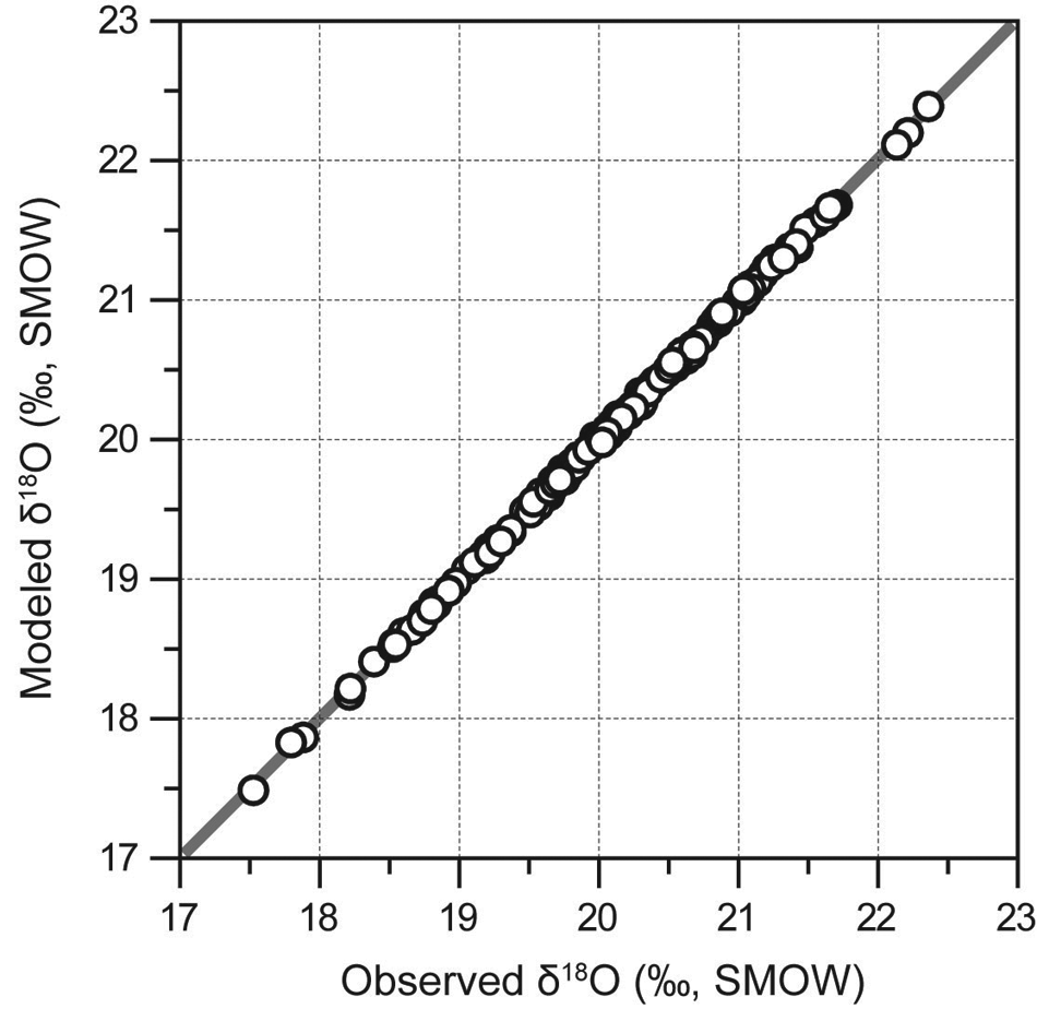
Scatter plot of the observed versus predicted peat cellulose δ¹⁸O data. Solid line shows the 1:1 relationship

The reliable reconstructions of climate for the past rely on an appropriate understanding of the relationship between climate and the proxies. This relationship should be formulated using a complex deterministic model instead of a simplistic statistical equation. The advantage of involving process-based models in palaeoclimate reconstruction is significant in several aspects. First, it could ensure a better understanding of the proxies mechanistically. Second, it is able to account for the complications that may be intractable using the transfer function method. Finally and most importantly, human disturbance may bias the statistical relationship between proxy and climate variables in terms of transfer function, but it could not alter the underlying physics that governs the formation of the fossil proxy records. However, there are only very a few kinds of palaeoclimate proxy that can be characterized using process-based models to date, and these models may be incomplete with some processes not being well understood and properly parameterized. Therefore, one of the major research targets in the future is to improve the understanding of the underlying physical processes so as to develop mechanistic models for most of the proxies. Another important caveat with this method is the dilemma between model complexity and computation cost. Mechanistic models covering the full spectrum of the processes involved in generating the proxies are preferable for the inverse proxy modeling. However, increasing the complexity of the models would inevitably increase the computational time. If a tremendously complicated model is incorporated, the inversion could turn out to be computationally intractable.

Concluding remarks

Within the Bayesian paradigm, we are able to reconstruct climate changes on the eastern Tibetan Plateau during the last 6000 years quantitatively by integrating a peat cellulose δ¹⁸O record with a process-based model of oxygen isotope fractionation in plant cellulose. Our results indicate that, to a large extent, the observed variation of the δ¹⁸O record reflects the changes in the oxygen isotopic composition of soil water, which appears to be a function of precipitation amount. Compared with hydrology, temperature and humidity have little influence on the oxygen isotopic fractionation of leaf water. This conforms the prevailing notion that the δ¹⁸O records in monsoonal areas should be primarily interpreted in terms of the ‘amount effect’.

The forefront of palaeoclimatological studies requires the development of not only reliable proxies of climate variables, but also powerful methods that can be used to integrate these proxy records across broad spectra. The inverse proxy modeling stands out as an excellent method for quantitative palaeoclimate reconstruction, because deterministic models and proxy records are integrated in a unified framework. This model–data fusion technique fundamentally differs from the traditional transfer function approach, and it represents a conceptual innovation in palaeoclimatological studies. This worked example also shows the promise of Bayesian statistics in quantitative palaeoclimatology. It not only offers a mathematical feasibility to solve the ill-posed inverse problems, but also provides an effective approach to quantifying the uncertainty of the inferred palaeoclimate data.

Footnotes

Appendix 1. Prior probability distribution of parameters

We choose a weakly informative prior probability distribution for parameter vector θ, given that their values are completely unknown for the past. The prior probability distributions of δ¹⁸O_s, T, and h are set to be uniform (UNIF) supported on a specific interval:

(A1)

f (δ^{18} O_{s}) = U N I F (- 20 - 5)

(A2)

f (T) = U N I F (0, 6)

(A3)

f (h) = U N I F (0, 1)

The prior of σ² follows Jeffreys’ distribution:

(A4)

f (σ^{2}) = \frac{1}{σ^{2}}

Appendix 2. Reversible jump and the acceptance probability

Draw a random number λ from the proposal distribution $q (λ) = 1 / λ, λ \in [\frac{1}{ρ}, ρ]$ , where ρ is a positive real number. We define a bijective transformation for T, h, and λ:

(A5)

{\begin{cases} T^{'} = T \times λ \\ h^{'} = h / λ \\ λ^{'} = 1 / λ \end{cases}

Therefore, the acceptance probability for this reversible jump move becomes:

(A6)

ω = \frac{π (y | δ^{18} O_{s}, T^{'}, h^{'}, σ^{2})}{π (y | δ^{18} O_{s}, T, h, σ^{2})} \times \frac{q (λ | λ^{'})}{q (λ^{'} | λ)} \times | J |

where J is the Jacobian of the transformation, which is defined as:

(A7)

J = | \frac{\partial (T^{'}, h^{'}, λ^{'})}{\partial (T, h, λ)} |

Appendix 3. Marginal posterior probability distribution of δ 18 O s,and σ 2

Equation (13) is rearranged to solve for δ¹⁸O_s yielding a truncated multivariate normal (MVN) distribution:

(A8)

\begin{array}{l} f (δ^{18} O_{s} | y, T, h, σ^{2}) = {(\frac{1}{2 π σ^{2}})}^{\frac{L}{2}} \exp [- \frac{{‖ y - δ^{18} O_{c} (θ) ‖}^{2}}{2 σ^{2}}] \times f (δ^{18} O_{s}) \\ = {(\frac{1}{2 π σ^{2}})}^{\frac{L}{2}} \exp [- \frac{{‖ δ^{18} O_{s} - E ‖}^{2}}{2 σ^{2}}] \times f (δ^{18} O_{s}) \\ M V N (E, Θ) \times I (δ^{18} O_{s}) \end{array}

where: E = y − (1−f₀)×(ε_eq+ε_k)×(1−h)−ε₀ is the mean vector; Θ = σ²I_L×L is the positive definite covariance matrix; I(δ¹⁸O_s) is an indicator function defined as:

(A9)

I (δ^{18} O_{s}) = {\begin{cases} 1, δ^{18} O_{s} \in (- 20, - 5) \\ 0, otherwise \end{cases}

A straightforward use of the Bayesian theorem yields an inverse Gamma (IG) distribution for the marginal posterior of σ²:

(A10)

f (σ^{2} | y, θ) \propto f (y | θ, σ^{2}) \times f (σ^{2}) \propto {(\frac{1}{σ^{2}})}^{\frac{L}{2} + 1} \exp [- \frac{{‖ y - δ^{18} O_{c} (θ) ‖}^{2}}{2 σ^{2}}] I G (\frac{L}{2}, \frac{{‖ y - δ^{18} O_{c} (θ) ‖}^{2}}{2})

Acknowledgements

We are grateful to Dr X. Hai for providing us with the Hongyuan peat oxygen isotope data. Our gratitude is also extended to the two anonymous reviewers for their constructive comments and suggestions.

S.-Y. Yu would like to thank the 100-Talents Program and the Strategic Priority Research Program (Grant No. XDA05120401) of the Chinese Academy of Sciences as well as the National Science Foundation of China (grant no. 41023006) for funding this work.

References

Araguás-Araguás

Froehlich

Rozanski

(1998) Stable isotope composition of precipitation over southeast Asia. Journal of Geophysical Research 103: 721–728.

Berger

Loutre

(1991) Insolation values for the climate of the last 10 million years. Quaternary Science Reviews 10: 297–317.

Bhattacharya

(2006) A Bayesian semiparametric model for organism based environmental reconstruction. Environmetrics 17: 763–776.

Birks

HJB

(1995) Quantitative palaeoenvironmental reconstructions. Statistical Modelling of Quaternary Science Data. Technical Guide 5: 161–254.

Blaauw

Bennett

Christen

(2010) Random walk simulations of fossil proxy data. The Holocene 20: 645–649.

Brenninkmeijer

CAM

Van Geel

Mook

(1982) Variations in the D/H and ¹⁸O/¹⁶O ratios in cellulose extracted from a peat bog core. Earth and Planetary Science Letters 61: 283–290.

Bryson

Kutzbach

(1974) On the analysis of pollen–climate canonical transfer functions. Quaternary Research 4: 162–174.

Burk

Stuiver

(1981) Oxygen isotope ratios in trees reflect mean annual temperature and humidity. Science 211: 1417–1419.

Cowling

Sykes

(1999) Physiological significance of low atmospheric CO₂ for plant–climate interactions. Quaternary Research 52: 237–242.

10.

Craig

Gordon

(1965) Deuterium and oxygen-18 variations in the ocean and the marine atmosphere. In: Tongiorgi

(ed.) Proceedings of a Conference on Stable Isotopes in Oceanographic Studies and Paleotemperatures. Spoleto, Italy, 9–130.

11.

Dansgaard

(1964) Stable isotopes in precipitation. Tellus 16: 436–468.

12.

Dongmann

Nürnberg

Förstel

Wagener

(1974) On the enrichment of H₂¹⁸O in the leaves of transpiring plants. Radiation and Environmental Biophysics 11: 41–52.

13.

Epstein

Yapp

(1977) Isotope tree thermometers. Nature 266: 477–478.

14.

Farquhar

Gan

(2003) On the progressive enrichment of the oxygen isotopic composition of water along a leaf. Plant Cell and Environment 26: 801–820.

15.

Garreta

Miller

Guiot

Hély

Brewer

Sykes

. (2010) A method for climate and vegetation reconstruction through the inversion of a dynamic vegetation model. Climate Dynamics 35: 371–389.

16.

Gebbie

Huybers

(2006) Meridional circulation during the Last Glacial Maximum explored through a combination of South Atlantic δ¹⁸O observations and a geostrophic inverse model. Geochemistry, Geophysics, Geosystems 7: Q11N07, doi:10.1029/2006GC00138310.1029/2006GC001383.

17.

Gebka

Mosbrugger

Schilling

Utescher

(1999) Regional-scale palaeoclimate modelling on soft proxy-data basis – An example from the Upper Miocene of the Lower Rhine Embayment. Palaeogeography, Palaeoclimatology, Palaeoecology 152: 225–258.

18.

Gilks

Richardson

Spiegelhalter

(1996) Markov Chain Monte Carlo in Practice. London: Chapman & Hall.

19.

Gray

Thompson

(1976) Climatic information from ¹⁸O/¹⁶O ratios of cellulose in tree rings. Nature 262: 481–482.

20.

Guiot

(1990) Methodology of the last climatic cycle reconstruction in France from pollen data. Palaeogeography, Palaeoclimatology, Palaeoecology 80: 49–69.

21.

Guiot

Torre

Jolly

Peyron

Boreux

Cheddadi

(2000) Inverse vegetation modeling by Monte Carlo sampling to reconstruct palaeoclimates under changed precipitation seasonality and CO₂ conditions: Application to glacial climate in Mediterranean region. Ecological Modelling 127: 119–140.

22.

Guiot

Garreta

Hatte

Magny

(2009) A few prospective ideas on climate reconstruction: From a statistical single proxy approach towards a multi-proxy and dynamical approach. Climate of the Past 5: 571–583.

23.

Gupta

Anderson

Overpeck

(2003) Abrupt changes in the Asian southwest monsoon during the Holocene and their links to the North Atlantic Ocean. Nature 421: 354–357.

24.

Hargreaves

Annan

(2002) Assimilation of paleo-data in a simple Earth system model. Climate Dynamics 19: 371–381.

25.

Haslett

Whiley

Bhattacharya

Salter-Townshend

Wilson

Allen

JRM

. (2006) Bayesian palaeoclimate reconstruction. Journal of the Royal Statistical Society-Series A 169: 395–438.

26.

Hatté

Guiot

(2005) Palaeoprecipitation reconstruction by inverse modelling using the isotopic signal of loess organic matter: Application to the Nußloch loess sequence (Rhine Valley, Germany). Climate Dynamics 25: 315–327.

27.

Hatté

Rousseau

Guiot

(2009) Climate reconstruction from pollen and δ¹³C records using inverse vegetation modeling – Implication for past and future climates. Climate of the Past 5: 147–156.

28.

Heinze

Hasselmann

(1993) Inverse multiparameter modeling of paleoclimate carbon-cycle indexes. Quaternary Research 40: 281–296.

29.

Helliker

Ehleringer

(2002) Grass blades as tree rings: Environmentally induced changes in the oxygen isotope ratio of cellulose along the length of grass blades. New Phytologist 155: 417–424.

30.

Hong

Liu

Lin

Yasuyuki

Leng

Wang

. (2009) Temperature evolution from the ¹⁸O record of Hani peat, Northeast China, in the last 14000 years. Science in China Series D: Earth Sciences 52: 952–964.

31.

Hong

Jiang

Liu

Zhou

Beer

. (2000) Response of climate to solar forcing recorded in a 6000-year d¹⁸O time-series of Chinese peat cellulose. The Holocene 10: 1–7.

32.

Hopcroft

Gallagher

Pain

Fang

(2009) Three-dimensional simulation and inversion of borehole temperatures for reconstructing past climate in complex settings. Journal of Geophysical Research-Earth Surface 114: F02019, doi:02010.01029/02008JF00116502010.01029/02008JF001165.

33.

Huntley

Prentice

(1988) July temperatures in Europe from pollen data, 6000 years before present. Science 241: 687–690.

34.

Huybers

Gebbie

Marchal

(2007) Can paleoceanographic tracers constrain meridional circulation rates? Journal of Physical Oceanography 37: 394–407.

35.

Imbrie

Kipp

(1971) A new micropaleontological method for quantitative paleoclimatology: Application to a Late Pleistocene Carribean core. In: Turekian

(ed.) The Late Cenozoic Glacial Ages. New Haven: Yale University Press, 71–181.

36.

Jackson

Williams

(2004) Modern analogs in Quaternary paleoecology: Here today, gone yesterday, gone tomorrow? Annual Review of Earth and Planetary Sciences 32: 495–537.

37.

Kühl

Gebhardt

Litt

Hense

(2002) Probability density functions as botanical–climatological transfer functions for climate reconstruction. Quaternary Research 58: 381–392.

38.

Korhola

Vasko

Toivonen

HTT

Olander

(2002) Holocene temperature changes in northern Fennoscandia reconstructed from chironomids using Bayesian modelling. Quaternary Science Reviews 21: 1841–1860.

39.

LeGrand

Wunsch

(1995) Constraints from paleotracer data on the North Atlantic circulation during the last glacial maximum. Paleoceanography 10: 1011–1046.

40.

Ménot-Combes

Burns

Leuenberger

(2002) Variations of ¹⁸O/¹⁶O in plants from temperate peat bogs (Switzerland): Implications for paleoclimatic studies. Earth and Planetary Science Letters 202: 419–434.

41.

Majoube

(1971) Oxygen-18 and deuterium fractionation between water and steam. Journal de Chimie Physique et de Physico-Chimie Biologique 68: 1423–1436.

42.

McKeague

Nicholls

Speer

Herbei

(2005) Statistical inversion of South Atlantic circulation in an abyssal neutral density layer. Journal of Marine Research 63: 683–704.

43.

Mosbrugger

Utescher

(1997) The coexistence approach – A method for quantitative reconstructions of Tertiary terrestrial palaeoclimate data using plant fossils. Palaeogeography, Palaeoclimatology, Palaeoecology 134: 61–86.

44.

Raffalli-Delerce

Masson-Delmotte

Dupouey

Stievenard

Breda

Moisselin

(2004) Reconstruction of summer droughts using tree-ring cellulose isotopes: A calibration study with living oaks from Brittany (western France). Tellus B 56: 160–174.

45.

Rajver

Safanda

Shen

(1998) The climate record inverted from borehole temperatures in Slovenia. Tectonophysics 291: 263–276.

46.

Robertson

Lucy

Baxter

Pollard

Aykroyd

Barker

. (1999) A kernel-based Bayesian approach to climatic reconstruction. The Holocene 9: 525–530.

47.

Roden

Lin

Ehleringer

(2000) A mechanistic model for interpretation of hydrogen and oxygen isotope ratios in tree-ring cellulose. Geochimica et Cosmochimica Acta 64: 21–35.

48.

Rousseau

Hatt

Guiot

Duzer

Schevin

Kukla

(2006) Reconstruction of the Grande Pile Eemian using inverse modeling of biomes and d¹³C. Quaternary Science Reviews 25: 2806–2819.

49.

Tarantola

(2005) Inverse Problem Theory and Methods for Model Parameter Estimation. Philadelphia: Society for Industrial Mathematics.

50.

Toivonen

HTT

Mannila

Korhola

Olander

(2001) Applying Bayesian statistics to organism-based environmental reconstruction. Ecological Applications 11: 618–630.

51.

Vasko

Toivonen

HTT

Korhola

(2000) A Bayesian multinomial Gaussian response model for organism-based environmental reconstruction. Journal of Paleolimnology 24: 243–250.

52.

Wang

Cheng

Edwards

Kong

. (2005) The Holocene Asian monsoon: Links to solar changes and North Atlantic climate. Science 308: 854–857.

53.

Widmann

Goosse

van der Schrier

Schnur

Barkmeijer

(2010) Using data assimilation to study extratropical Northern Hemisphere climate over the last millennium. Climate of the Past 6: 627–644.

54.

Wolfe

(1995) Paleoclimatic estimates from Tertiary leaf assemblages. Annual Review of Earth and Planetary Sciences 23: 119–142.

55.

Guiot

Brewer

Guo

(2007a) Climatic changes in Eurasia and Africa at the last glacial maximum and mid-Holocene: Reconstruction from pollen data using inverse vegetation modelling. Climate Dynamics 29: 211–229.

56.

Guiot

Brewer

Guo

Peng

(2007b) Dominant factors controlling glacial and interglacial variations in the treeline elevation in tropical Africa. Proceedings of the National Academy of Sciences 104: 9720–9724.

57.

Wunsch

(2003) Determining paleoceanographic circulations, with emphasis on the Last Glacial Maximum. Quaternary Science Reviews 22: 371–385.

58.

Hong

Lin

Zhu

Hong

Jiang

(2006) Temperature responses to quasi-100-yr solar variability during the past 6000 years based on d¹⁸O of peat cellulose in Hongyuan, eastern Qinghai-Tibet plateau, China. Palaeogeography, Palaeoclimatology, Palaeoecology 230: 155–164.

59.

Yakir

DeNiro

(1990) Oxygen and hydrogen isotope fractionation during cellulose metabolism in Lemna gibba L. Plant Physiology 93: 325–332.

60.

Zhang

Nakawo

Yao

Han

Xie

(2002) Variations of stable isotopic compositions in precipitation on the Tibetan Plateau and its adjacent regions. Science in China Series D: Earth Sciences 45: 481–493.

61.

Zhang

Yao

Nakawo

(2001) Oxygen-18 in present-day precipitation on the Tibetan Plateau. Science in China Series E: Technological Sciences 44: 41–47.

Quantitative palaeoclimate reconstruction as an inverse problem: A Bayesian inference of late-Holocene climate on the eastern Tibetan Plateau from a peat cellulose δ 18 O record

Abstract

Keywords

Introduction

Basic concepts and theoretical framework of the inverse proxy modeling method

Model, data, and algorithm

Model of oxygen isotope fractionation in plant cellulose

Description of the peat cellulose δ18O record

The Hasting-within-Gibbs algorithm

Results

Discussion

Concluding remarks

Footnotes

Appendix 1. Prior probability distribution of parameters

Appendix 2. Reversible jump and the acceptance probability

Appendix 3. Marginal posterior probability distribution of δ 18 O s,and σ 2

Acknowledgements

References

Description of the peat cellulose δ¹⁸O record