Holocene development and geomorphic processes at Omnsbreen,southern Norway: Evidence for glacier

Abstract

Omnsbreen is a small (<0.5 km²) and degrading glacier situated at the regional lower limit of present-day permafrost distribution and glaciation. At present, the existence of Omnsbreen is mainly dependent on wind-borne snow redistributed by the prevailing westerly winter-wind, and lies in an area of marginal permafrost occurrence. During the ‘Little Ice Age’ (LIA) both the glacier and the distribution of permafrost in the area reached their maximum late-Holocene areal extents. The first occurrence of Omnsbreen is recorded in sediment cores retrieved from a proglacial lake and dated at ad 1425, and marks the onset of the local LIA. Reconstruction of the maximum LIA extent by means of geomorphic indicators revealed a size of 7.1 km², a volume of more than 0.25 km³ and a maximum glacier thickness of 110 m. Since the LIA Omnsbreen has been reduced by more than 90% in area. Omnsbreen retreated rapidly from its LIA maximum, which we suggest was determined by the shape of the glacier, filling up the valley, and hence being unable to accumulate wind-borne snow. Prominent glacier marginal landforms are absent along the maximum LIA extent of Omnsbreen. We propose that the lack of glacier marginal landforms in this case is indicative of a cold glacier margin, and that the landscape evolution in maritime and marginal permafrost regions is characterised as being closely connected with glacial activity.

Keywords

geomorphology glacier glacier–permafrost interactions ‘Little Ice Age’Omnsbreen permafrost

Introduction

Glacial activity has served as one of the main sources for palaeoclimatic reconstructions of the Late Pleistocene and Holocene in Scandinavia. In addition, permafrost holds a strong climate signal, but this signal is harder to measure and observe, as permafrost is thermally defined and a subsurface phenomenon. Traditionally, landforms and processes related to glaciers and permafrost are treated as separate research fields in the cryospheric literature. However, in nature, these phenomena commonly coexist and have the potential to interact (Berthling and Etzelmüller, 2011; Etzelmüller and Hagen, 2005, Haeberli, 2005; Shumskii, 1964). Most glaciers in Norway disappeared during the Holocene Thermal Maximum (HTM; in Scandinavia at 9000–5000 yr BP), and reappeared following this warm period as a Neoglacial phenomenon (Nesje, 2009; Nesje et al., 2005, 2008). The Holocene history of permafrost is generally less studied in Norway than the glacier variations, which is also the case globally (Harris and Murton, 2005). A recent study (Lilleøren et al., 2012) suggests that the Holocene mountain permafrost variation in Norway in many ways resembles the glacial history. However, unlike the glaciers, permafrost at the highest altitudes has presumably existed continuously since deglaciation, and probably also beneath cold-based parts of the Fennoscandian ice sheet (Kleman and Borgström, 1994; Kleman and Hättestrand, 1999; Sollid and Sørbel, 1988, 1994). The Holocene permafrost most likely reached both its maximum spatial extent and depth during the ‘Little Ice Age’ (LIA) underlying areas which are currently thawed (Gisnås et al., 2013), and likewise some glaciers might be looked upon as strictly LIA phenomena.

Whereas glaciers are defined as part of the hydrosphere, permafrost is defined as a part of the lithosphere (Shumskii, 1964), with the thermal regime as the common denominator (Berthling and Etzelmüller, 2011; Etzelmüller and Hagen, 2005). Permafrost and glaciers commonly coexist and interact in regions where the lower mountain permafrost occurrence is situated well below the equilibrium-line altitude (ELA) of glaciers (cf. Etzelmüller and Hagen, 2005). Hence, glaciers and mountain permafrost coexist in areas that are sufficiently high and thus cold enough for permafrost to occur, while still receiving the necessary amount of precipitation to maintain glaciers (cf. the ‘cryosphere model’; Haeberli and Burn, 2002). In Norway the mountain permafrost altitude (MPA) decreases from west towards east, while the opposite is the case for the ELA (Etzelmüller et al., 2003a; King, 1986), and glacier–permafrost interactions occur in central mountain regions such as the Jotunheimen massif, where the two zones overlap. In the outskirts of such zones, where the environment is sensitive to permafrost and/or glacier formation, the simplest relationship is that heavy winter (accumulation season) snowfall produces glaciers whereas low winter snowfall favours permafrost (Harris and Corte, 1992). In this strictest sense, permafrost aggradation and glacier formation and existence are mutually exclusive processes, and should not occur simultaneously whenever any of these phenomena are close to marginal conditions. In warm permafrost environments the distribution of snow can be decisive of the permafrost extent (Smith and Riseborough, 2002).

In areas of permafrost, glaciers provide a thermal offset between the ground surface and the atmosphere. Depending on winter air temperatures, glacier dynamics and snow cover over the summer, parts of the glacier will remain cold, frozen to its bed and preserve sub-zero ground temperatures. The thickness of the cold ice may vary from less than 10 m in marginal permafrost areas such as reported from the Finse area (e.g. Liestøl, 2000), via several tens of meters on glaciers on Svalbard (Björnsson et al., 1996) to hundreds of meters in the large ice sheets of Antarctica and Greenland with cold firn accumulation (Paterson, 1994). In areas with warm firn and summer melting, typical for most glaciers in Norway and Svalbard, meltwater will penetrate the firn areas and refreeze, leading to temperate conditions in the firn zone. Ice below the ELA will be colder because of meltwater evacuation from the impermeable ice surface, leading to temperature inversions in the glacier (i.e. polythermal glaciers; Liestøl, 1977). Independent of the climatic situation also small, initially temperate glaciers will become cold or polythermal during retreat owing to energy loss when meltwater escapes the increasing ablation area, and the corresponding firn areas are reduced (Hock, 2005; Paterson, 1994). Locally, permafrost will develop in connection to such retreating glaciers. The latter is also the case for small, long-term stable ice patches, which can be considered a permafrost indication (Haeberli, 2000).

At present, most of the glaciers in Norway decrease in volume as a response to the ongoing atmospheric warming (e.g. Andreassen et al., 2010; Dyurgerov, 2003; Nesje et al., 2008), a situation that has lasted since the late-Holocene glacial maximum during the LIA (mid-18th century). Mass loss has accelerated in recent decades (e.g. Andreassen et al., 2005). Several processes are involved in such glacial retreats. In addition to changes in summer temperature and winter precipitation, an important factor is how wind-redistributed snow locally may control the existence and geometry of glaciers. Thus, individual glacier response to climate perturbations can vary considerably even within small geographical regions depending on glacier size, shape, aspect and local topography.

In this paper, we present a new investigation of the age, extent, volume and dynamics of Omnsbreen, a small glacier or glacieret north of Finse in southern Norway. This glacier is situated in an area where the lower glaciation limit and the lower limit of mountain permafrost overlap, located in a snow-rich maritime and relative mild climatic setting. We hypothesize that interactions between glaciers and permafrost provide important constraints for understanding Holocene landscape development in such an environment. The objective was first addressed by mapping and reconstructing the maximum glacier geometry, using geomorphological indicators. Further, the first appearance of the glacier during the late Holocene was constrained by analysing lacustrine sediment cores from a proglacial lake (Omnsvatnet) northeast of Omnsbreen. Finally, a permafrost model was used to examine the probable ground thermal regime in the area during the maximum extent of the glacier and at present.

Study area

The Omnsbreen glacier is situated approximately 5 km north of Finse, at the northwestern rim of the Hardangervidda high mountain plateau (Figure 1). At present, the glacier is a small (<0.5 km²) mountain glacier or glacieret (Cogley et al., 2011) existing close to or a little lower than the regional ELA (Andreassen et al., 2010) at around 1700 m a.s.l. mainly as a result of high local snow accumulation (Liestøl and Sollid, 1980). At present the remnants of Omnsbreen occupy elevations between 1500 and 1700 m a.s.l. Current glacier thickness and hence volume is unknown. During the LIA the glacier was considerable larger, and filled the entire north/south-trending valley where it at present only occupies parts of the western slope (Liestøl and Sollid, 1980). From the LIA maximum until around 1930 the glacier remained relatively stable in shape and size (Elven, 1978; Liestøl and Sollid, 1980). Between 1930 and 1985, however, the bulk of the glacier disappeared (Høgvard, 1987; Messel, 1971). Since then the glacier has lost mass at a lower rate, until recent years when the glacier apparently has stagnated at a fairly constant size (Figure 2). Most of the western maritime glaciers in Norway stopped retreating and even gained mass during the last part of the 1980s and throughout the 1990s, as a response to higher winter precipitation rates (Nesje and Matthews, 2012; Nesje et al., 2000, 2008). Omnsbreen is not surrounded by headwalls and neither currently or during its LIA maximum stage was extra-glacial debris added to the glacier surface.

Figure 1.

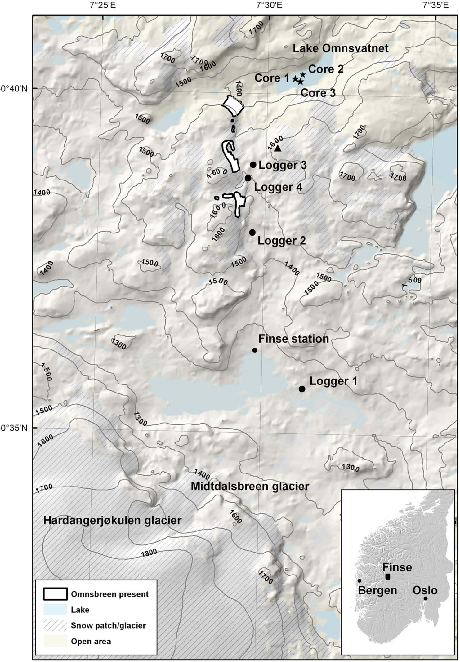
Key map of the Finse and Omnsbreen region. Miniature temperature datalogger sites (solid circles), core sites (stars) and the hill where R. Elven (1978) found plant remnants (triangle north of Logger 3) are marked.

Figure 2.

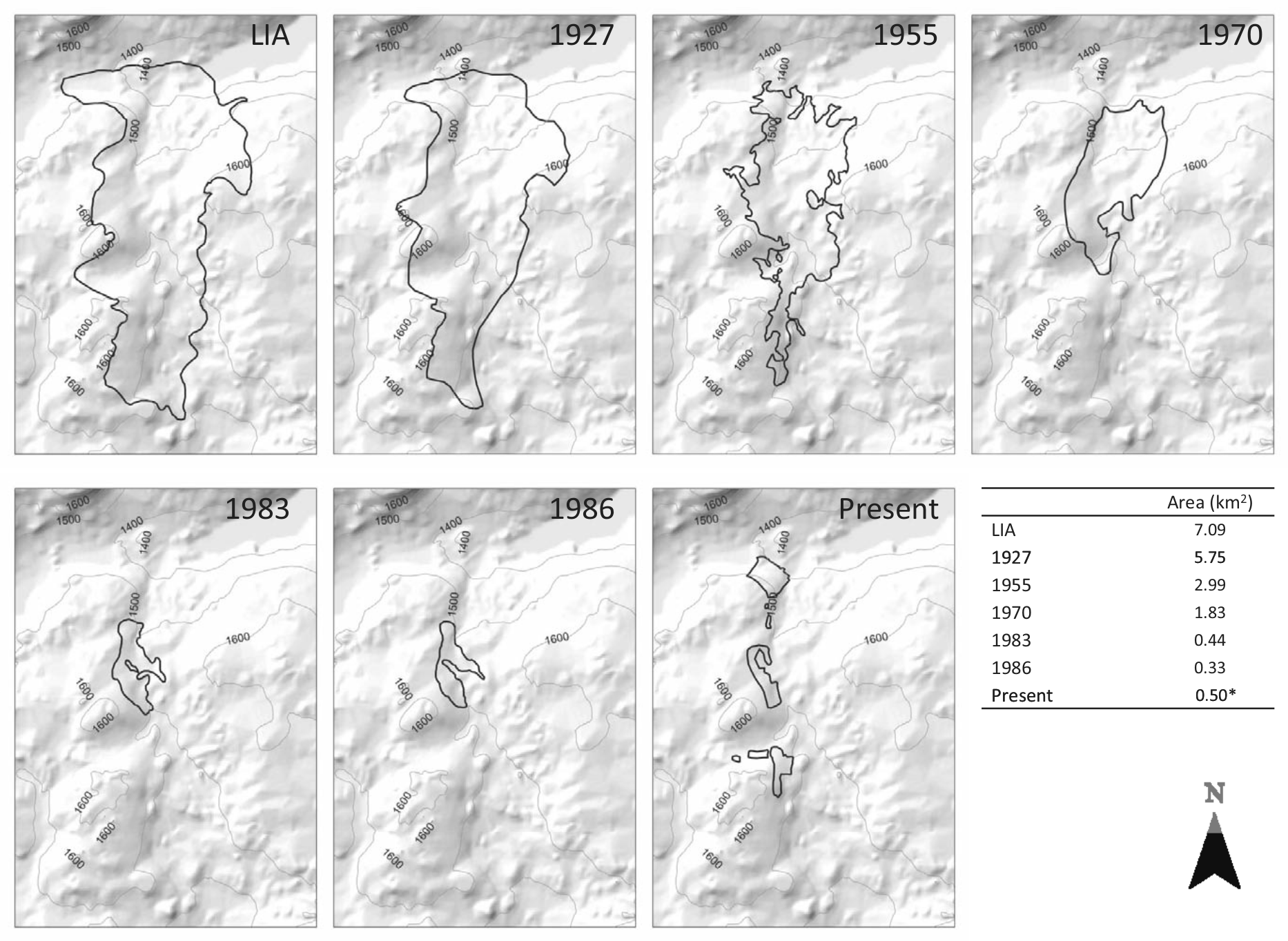
Development of the Omnsbreen glacier from its maximum extent until present. The maps are based on Høgvard (1987) and Messel (1971). The table gives calculated areas during the different times. The map indicating the present area includes areas that were excluded on maps from 1983 and 1986, and hence give a larger area than the previous years.

Climatically, the Finse area is situated in a transition zone between the maritime western coast and the more continental eastern parts of Norway, and has a high mountain climate. Precipitation and temperature, and hence glaciers, in these western mountain areas are affected by the North Atlantic Oscillation (NAO), as for example evident by the glacier advances during the 1990s (Nesje et al., 2008). At c. 1220 m a.s.l., about 300 m lower than Omnsbreen, the mean annual air temperature (MAAT) is −2.1°C (1971–2000), and the mean annual precipitation (MAP) in the same period is 1030 mm (DNMI, 2007). Maximum snow thickness in the region is between 200 and 400 cm (SeNorge, 2011).

The bedrock in the Omnsbreen catchment is dominated by phyllite of both the dark mica-rich type and the lighter quartz-rich type. Phyllite is a pholiated, easily weathered and erodable metamorphosed slate (Sigmond and Askvik, 2008).

Permafrost in southern Norway is present in high-mountain areas, with a general lower limit of approximately 1500–1600 m a.s.l. and is mainly concentrated in a 50–100 km wide belt from Hallingskarvet as its southern margin and widens following the main mountain range from SW to NE (Etzelmüller et al., 2003a). Hence, the Finse mountain area is situated close to the present lower limit of mountain permafrost. Permafrost models for Norway (e.g. Etzelmüller et al., 2001, 2003a; Gisnås et al., 2013), suggest permafrost occurrence both in Hallingskarvet and at the margins of Omnsbreen and Hardangerjøkulen. Further, modelling indicates that larger areas were underlain by permafrost during the LIA (Figure 3). Indications of permafrost in the Finse area have been reported from Midtdalsbreen, a northern outlet glacier of Hardangerjøkulen, where cold ice (<0°C) and frozen subglacial till have been observed along the margin of the glacier lobe (Liestøl and Sollid, 1980). Also, DC-resistivity soundings on mountain areas surrounding Finse at above 1450 m a.s.l. and in front of Midtdalsbreen indicate permafrost at snow-free sites (Etzelmüller et al., 2003b). In addition, thermistor strings installed in Omnsbreen in March 1985 showed that the uppermost 2–3 m of ice never reached temperatures at the pressure melting point, while a positive temperature gradient into the ice indicated pressure melting point conditions at the glacier bed (Høgvard, 1987).

Figure 3.

Permafrost distribution in southern Norway modeled using CryoGRID1.0 (Gisnås et al. 2013). Blue and purple areas indicate present permafrost distribution, while yellow areas simulate the ‘Little Ice Age’ distribution. Black circles indicate ice-cored moraines, while the square on the inlet map is the same area as Figure 1 (colour figure available online).

Methods

Climate data analysis

Air, ground and surface temperatures were measured hourly using TinyTag© miniature temperature loggers (MTDs) with an accuracy of ±0.1°C (Figure 1). The loggers measuring air temperature were installed in ventilated stone cairns at snow free locations, and up to 50 cm above ground. Ground sensors were placed down to 100 cm. Meteorological data were otherwise obtained from the Norwegian Meteorological Office (DNMI), mainly from two different meteorological stations situated at Finse (‘Finse’, 1904–1924 and 1969–1994, and ‘Finsevatn’, 2002–present). Because of the poor temporal coverage of the data, records from three different meteorological stations in Bergen were used to interpolate the data sets from Finse. The Bergen data sets contain temperature data from 1861 and precipitation data from 1904.

Based on temperature data, a simple degree-day model was used over the Omnsbreen area to model glacier ablation, following the relationship given by Bamber and Payne (2004):

N = β T_{DDT}

(1)

where N is the total ablation, β is the degree-day factor (mm/K per day) and T_DDT is the sum of all positive degree-days in the period of interest.

The lapse rate between Finse and Omnsbreen was calculated from the measured temperatures at Omnsbreen for the specific time period 2006–2011, and the degree-day factor (β = 5.5 mm/K per day) was calculated by summer balance measurements for the period 1966–1969 done by Messel (1971).

Wind speed and direction were measured at the meteorological stations at Finse, and compared with the longer series from Bergen (Figure 4a–c). In addition the orientation of winter surface landforms in snow such as zastrugi (Figure 4d) (Shumskii, 1964), cornices on top of slopes, and lee side accumulations (Figure 4e) in the surroundings of Omnsbreen were mapped. While small-scale landforms such as zastrugi give information on the wind direction for the past hours or days, the larger landforms indicate weekly or monthly wind direction.

Figure 4.

Wind diagrams from (a) Bergen (1886–2011), (b) Finse (1982–1994), and (c) Finsevatn (2002–2011) (all wind speed units in m/s), (d) small-scale snow-surface forms, zastrugi, showing the wind-direction from the last few days (picture taken towards south), and (e) lee-side wind deposits indicating the main winter-wind direction (picture taken towards north) (colour figure available online)

Geomorphological mapping

Landforms observed in the glacial zone that are indicative of glacier movement include striae, crag-and-tails, boulder tracks in the till, drumlins, flutings and eskers (Figure 5). In addition, several recession stages of Omnsbreen produced glacier-dammed lakes and associated shorelines and spillways (Høgvard, 1987; Liestøl and Sollid, 1980). Finally, ‘domino’-structures of bedrock piles were interpreted as ice-marginal or glacier-overridden features (Figures 6e and f). The ‘domino’-structures are caused by glacier ice movement against exposed slabs of layered phyllite bedrock. The phyllite dip 5–10° towards the east and at places where the LIA Omnsbreen had an easterly ice flow component, protruding slabs of phyllite were broken off and rotated in the direction of ice flow. This process produced a landform pattern that visually resembles a collapsed row of domino bricks. These rotated slabs of phyllite are difficult to explain other than by glacier overriding, especially where they have been rotated upslope. They are especially frequent along the eastern slope of the main valley Omnsdalen, and in the absence of moraines we have used the outermost occurrences of ‘domino’-structures to delimit the maximum LIA extension of Omnsbreen. Related landforms have been observed in the Scottish Cairngorm Mountains where toppling of tors is interpreted as an erosional effect of cold-based ice (Phillips et al., 2006).

Figure 5.

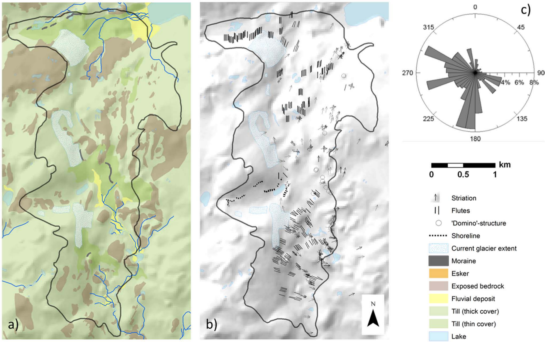
(a) Sediment map and (b) map of flutes, striae, shorelines and marginal landforms (‘domino’-structures) of the Omnsbreen area, and (c) striation orientation.

Figure 6.

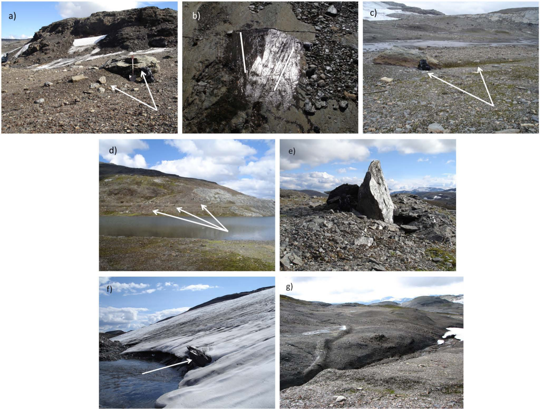
(a) Crag-and-tail landform in the northern part of the glacier marginal area, picture taken towards NE, (b) two crossing directions of striae, (c) example of a ploughing boulder in till in the southern part of the glacier marginal area, picture taken towards W, (d) successive relict shorelines above the present lake Omnstjern, picture taken towards NE, (e) ‘domino’-structure in the eastern marginal area, used to establish the glacier’s outline in its eastern margin, picture taken towards SSE, (f) ‘domino’-structure in making, below the central present glacier, picture taken towards S, and (g) moraine formed in a readvance in the central glacial foreland, picture taken towards SE.

Reconstruction of the glacier geometry and associated parameters

Based on landform mapping the outer limits of the LIA glacier geometry were established. First, we limited the previously glacierized zone based on the geomorphological map and in field. The rest of the procedure were performed in the ESRI software ArcMap©, first by digitizing surface contour lines at 25 m spacing based on the assumption that the steepest surface slope is aligned parallel to the direction of the glacier movement, thus the contour lines are oriented perpendicular to the direction of the striae, crag-and-tails and boulder tracks. The glacier surface was interpolated from elevation points at the glacier margin and the interpreted contour lines, using the ArcGIS-inbuilt ‘Topo to raster’-tool (Hutchinson, 1989; Hutchinson and Dowling, 1991). The surface slope was then calculated via the ‘Slope’-tool, and averaged over 500 m which correspond to 15 times the average glacier thickness (cf. Etzelmüller and Björnsson, 2000), following the suggestion in Nye (1965) for valley glaciers (averaging ten to twenty times). The volume between the LIA glacier surface and the terrain was calculated subtracting the LIA surface from the current DEM. The subglacial shear stress (τ) was calculated from the equation:

τ = F ρ g h \sin α

(2)

where F is a shape factor assigned to valley glaciers (we used 1), ρ is the ice density (900 kg/m³), g is the gravitation (9.81 m/s²), h is the glacier thickness and α is the surface slope (Nye, 1965; Paterson, 1994). A general ground resolution of 25 m was applied. The spatially distributed values of basal shear stress can be interpreted as a measure of glacier activity. Further, the strain rate (µ^.) of the ice is given by Glen’s flow law:

\dot{ε} = A^{τ n}

(3)

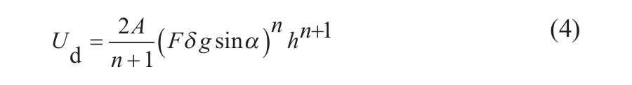
where A is a constant which decreases at lower temperatures and n is the flow law exponent, normally with a value close to 3 (Benn and Evans, 1998; Glen, 1955). The deformation velocity (U_d) is found by integrating the strain rate over the ice thickness, following Nye (1965):

U_{d} = \frac{2 A}{n + 1} {(F δ g \sin α)}^{n} h^{n + 1}

(4)

In addition to ice deformation, the glacier moved by basal sliding evident from landforms in the LIA glacier zone, even though not quantified here. Additional parameters such as annual ablation were calculated as:

b_{t} = d b / d H (H_{m} - H_{min})

(5)

where the mass balance gradient (db/dH) was given a value of 0.75 m w.e. per 100 m per year in accordance to nearby Midtdalsbreen, and the altitude range of the ablation area (H_m − H_min) as the difference between the approximated ELA (H_m) and the glacier snout (H_min). Further, response times were calculated as:

t_{resp} = h_{\max} / b_{t}

(6)

where h_max is the maximum glacier thickness, and the mean slope as α_m = arctan(ΔH/L₀), where ΔH is the total altitudinal range of the glacier and L₀ the full glacier length, all following Haeberli and Hoelzle (1995).

Lake sediment cores from Omnsvatnet

Three sediment cores were retrieved from Omnsvatnet (for locations, see Figure 1), using a modified piston corer (Nesje, 1992) and four sediment cores using a gravity corer (Renberg, 1991). The cores 1, 2 and 3 were 135 cm, 132 cm and 260 cm long, respectively, but the total sediment thickness in the lake is unknown. The sediment cores were further subjected to analyses of the weight-loss-on-ignition (LOI), dry bulk density (DBD), magnetic susceptibility (MS) (10^–⁵ SI) and grain-size variations (sedigraph). Three radiocarbon dates were obtained from macroscopic plant remains (Drepanocladus sp. and Salix sp. leaves at 50, 75 and 117 cm depth) and a ²¹⁰Pb series from the topmost sediments in core 2 were obtained to construct an age–depth relationship for the sediments deposited during the last ~2500 years in Omnsvatnet (Sægrov, 2006).

Modelling of ground thermal regime

For Norway a distributed permafrost model (CryoGRID1.0) has been implemented and is driven by 1 km² gridded snow and air temperature (Gisnås et al., 2013). The model is based on the TTOP-approach (cf. Smith and Riseborough, 1996), and simulates the relationship between climate and permafrost, which based on air temperature data defines the temperature at the top of permafrost or alternatively at the base of the seasonal frost (Smith and Riseborough, 1996, 2002). CryoGRID1.0 operates as a three-layer system: (1) the mean annual air temperature (MAAT), (2) the mean annual ground surface temperature (MAGST), and (3) the mean annual temperature at the top of the permafrost/base of the seasonal frozen layer (TTOP/MAGT), and requires scaling factors (n-factors) dependent on snow depth in winter and vegetation in summer to adjust air temperatures to ground temperatures. The climatic input data for CryoGRID1.0 is average degree-days over a chosen climatic period and the average snow depth. For a comprehensive model description and more details on input parameters, see Gisnås (2011).

CryoGRID1.0 was run for three different Holocene time periods representing different climate scenarios: (1) the present situation, (2) the LIA situation, and (3) the HTM situation (Lilleøren et al., 2012). For LIA and HTM the input degree-days were equally changed compared with the present situation for southern Norway, and for the LIA situation the annual snow depth was increased to 130% of the present situation (based on e.g. Bjune et al., 2004; Matthews et al., 2005; Nesje et al., 2001). The freezing and thawing degree-days were changed according to anomalies of winter and summer temperatures from the applicable MAAT. The Holocene MAATs were created primarily based on speleothem data (Lauritzen and Lundberg, 1999) compared with the surface temperature of the GISP2 ice core site (Alley et al., 1995; O’Brien et al., 1995), and adjusted with local Holocene summer temperature data compiled from numerous publications (summarized in Nesje, 2009, and discussed in detail in Lilleøren et al., 2012). The Holocene winter temperatures are expressed as regressions between modern MAAT and winter temperatures. Cells containing glaciers are masked from the model, which leads to empty areas where Omnsbreen is situated (i.e. Figure 2).

Results

Observations on temperature, lapse rates, wind and snow cover

The regressions between temperatures measured in Bergen and at Omnsbreen are slightly better than between Finse and Omnsbreen (r² = 0.91 and r² = 0.88 (N = 1475), respectively), in spite of the much closer distance. This is due to winter temperature inversions local to the Finse area, as the meteorological station at Finse measures lower air temperatures than the MTDs at Omnsbreen. Omnsbreen is freely exposed to circulating air masses, and the largest temperature inversions occur on cold and calm winter days. The average annual lapse rate is 0.0067°C/m both between Bergen and Omnsbreen and between Finse and Omnsbreen for the years of observations from Omnsbreen. The extrapolated MAAT series of Omnsbreen since 1862 shows a warming tendency towards modern time, however, 2010 is the sixth coldest year in the temperature data set, and the coldest year since 1919 (Figure 7). The general variations of the temperatures at Omnsbreen resemble global trends for the same time period (e.g. Brohan et al., 2006).

Figure 7.

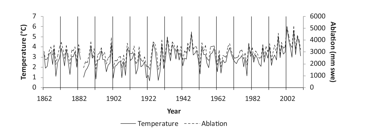
Ablation season air temperatures and modelled ablation in snow water equivalents at Omnsbreen for the years 1862 through 2010. Temperatures are extrapolated from air temperature measurements in Bergen for the same period.

Mapping of snow-cover surface forms as an indicator for wind direction demonstrated that the prevailing winter wind direction in the area is from west or slightly southwest, which is consistent with the most recent measurements in the Finse valley (Figure 4c). Here, a second component of the wind direction comes from the southeast, reproducing the orientation of the valley axis. In Bergen the same two dominant wind directions are present, i.e. northwesterly and east-southeasterly (Figure 4a). The valley where Omnsbreen is situated has a north–south orientation and snow transported by westerly winds today effectively accumulates on the valley’s east-facing slope. Wind directions measured at the meteorological station in the Finse valley show a shift in the dominating wind direction since the 1970s to present, from a wide directional spread during winter to a more consistent westerly wind flow since the early 1980s. This shift also coincides with the decelerating mass loss from the Omnsbreen glacier.

The degree-day model suggests increased ablation rates from c. 1985 on, a result that is not observed at Omnsbreen (Figure 7). This can be due to the general higher winter precipitation recorded in western Norway in the same period. Hence, there is no clear relationship between mass loss at Omnsbreen and the ablation rate from the degree-day model used here.

Glacial geomorphology at Omnsbreen

The LIA glaciated zone is characterized by apparently thick sediment depositions in topographic depressions surrounded by exposed bedrock. Sediments are both till and in situ weathered material from the highly pholiated phyllitic bedrock in the area. The general appearance is that of a recently deglaciated area, with typical glacial landforms such as striae, eskers, crag-and-tails, moraines, flutings and plough marks (Figure 5). The mentioned landforms occur frequently throughout the area (refer to Figure 6 for pictures of landforms). Terminal moraines were observed, though do not mark the maximum extent of the glacier, but rather re-advances within the glacial zone at later stages; which stages, however, are unclear. Relict shorelines at different levels were observed above Lake Omnstjern, indicating several former lake levels. Lateral meltwater channels were observed in a limited amount. Erosional landforms such as roche moutonnées occur in the area, and striations very frequently occur on exposed bedrock sites, and often with more than one direction (Figure 5c). ‘Domino’-structures occur frequently close to the current glacier margin and in the eastern LIA glacier zone.

Reconstruction of LIA glacier geometry and extent

The extent of Omnsbreen during the LIA is estimated from mapping of the geomorphological features previously listed. In the absence of a well-developed system of terminal moraines, we delimited the maximum glacier extent using other landforms, in particular radial striae and ‘domino’-structures. Thus, the extent of the glacier was interpreted based on dynamical criteria, where only zones with a clear indication of glacier movement were considered as formerly glaciated. It is likely that the margins of the dynamically active glacier were connected to firn areas that never underwent significant deformation, as the vegetation appearance of the two zones is not very different. Based on crossing directions of striae and tentative identification of striae pre-dating LIA at Omnsbreen, the initiation area of the glacier is interpreted to have been on the western slope of the valley, close to where the remnants of the glacier is situated today, and with initial movement towards the east more or less across the main valley orientation. However, when the glacier reached the eastern valley slope it was forced to diverge and flow south- and northwards and an ice divide developed. In the northern zone the valley slopes are steep and terminate in a flat plain leading into Lake Omnsvatn. In the steep part of the valley the glacier velocity was presumably high, resulting in correspondingly high shear stress on the substrata (Figure 8). The glacier itself might have terminated into the lake, or close to the present shoreline. In this area, the potential mapping error of the glacier extent is particularly high, as most ice marginal landforms probably have been removed by later fluvial erosion. In the southern zone of the main valley, the glacier terminated on a gentle slope towards the larger Finse valley, but did not reach all the way down. As the glacier grew, an ice divide that extended obliquely across the valley developed (see Figure 8). At this maximum stage the glacier behaved more like a plateau glacier than a valley glacier.

Figure 8.

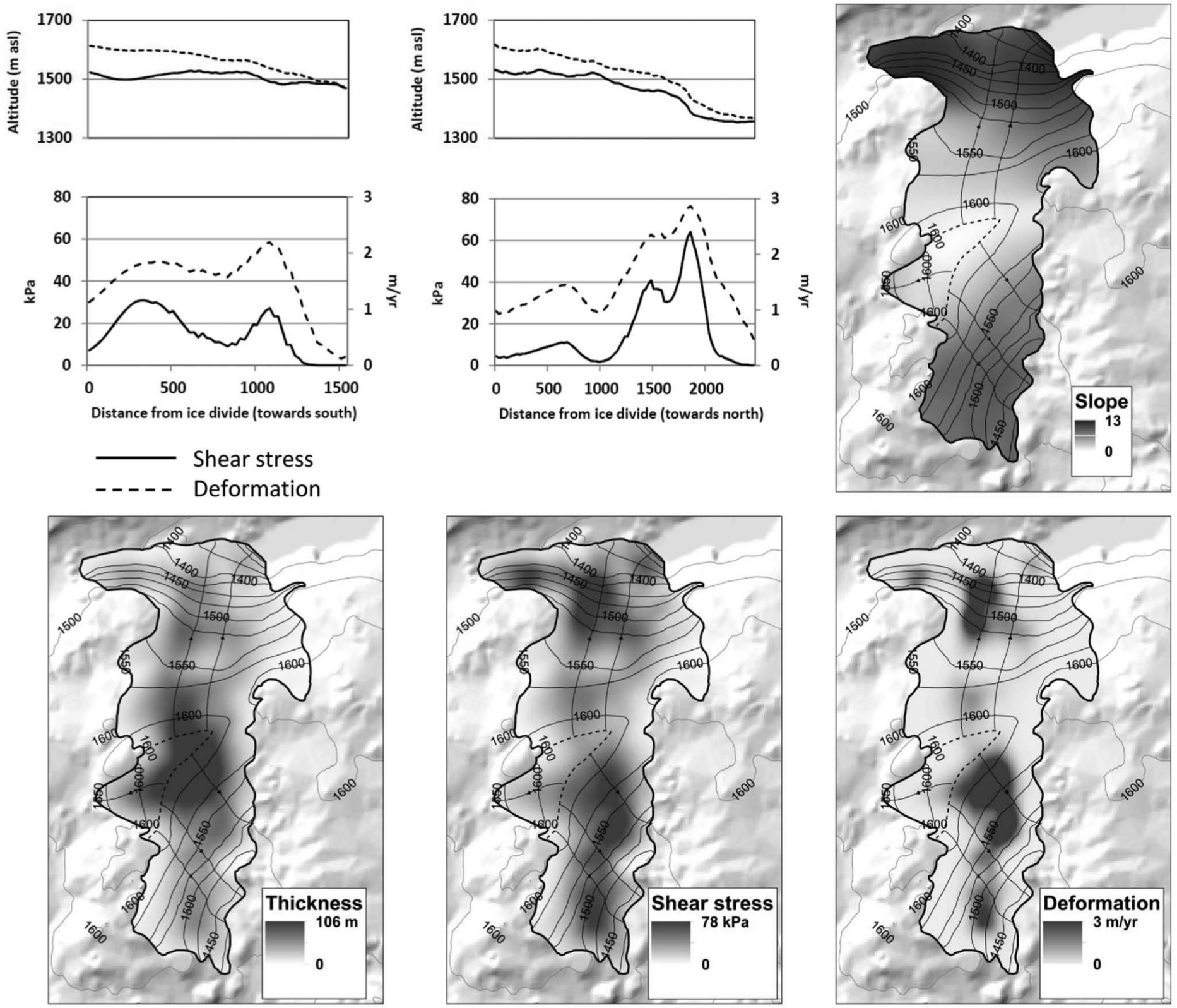
(a) Glacier thickness during the ‘Little Ice Age’, (b) glacier slope, (c) corresponding subglacial shear stress, and (d) deformation velocity. Flow lines (solid lines) and ice divide (dotted line) are indicated.

Based on our estimation this maximum area covered by the LIA glacier was c. 7.1 km², with an estimated maximum LIA thickness of 110 m. The interpreted LIA glacier surface has a maximum elevation of c. 1610 m a.s.l. and a minimum elevation of 1320 m a.s.l. The estimated ELA was then at c. 1530 m a.s.l. assuming a 60/40 relationship between area above and below the ELA (Haeberli et al., 2005). The total length of the glacier was c. 5 km, while the southern flowlines are c. 1.5 km and the northern flowlines c. 2.4 km dispersed from a fairly flat summit area (Table 1). The maximum calculated shear stress occurs in the northern zone of the LIA glacier, where the surface slope is high, close to where the northern remnant of Omnsbreen currently is situated. The values range up to 70 kPa, while the average values are around 25 kPa (Figure 8c). The annual deformation velocity is low, with maximum values at 3 m/yr, while major parts of the glacier deformed less than 1 m/yr (Figure 8d). Following Haeberli and Hoelzle (1995) the annual ablation of LIA Omnsbreen was 1.1 m w.e., however based on modern mass balance gradients. This value is in accordance with values measured at Midtdalsbreen. The response time of LIA Omnsbreen was estimated to c. 100 years. In Norway the maximum Holocene position of glaciers occurred during the LIA, and is usually dated to the mid-18th century. According to interpretations of the lake sediment record in Omnsvatnet (Sægrov, 2006), Omnsbreen reached its maximum LIA extent at around ad 1580, which is significantly earlier than other glaciers where such data exist, and following a period of retreat, reached another maxima at ad 1820, however, slightly less extensive than the first.

Table 1.

Parameters of Omnsbreen at LIA maximum and present, and change in the same period. At present Omnsbreen exists as fragments.

	LIA	Present	Change since LIA
Area (km²)	7.1	0.5	6.6
Volume (km³)	–	–	0.25
Average thickness (m)	–	–	32.1
Max thickness h_max (m)	110	c. 25	c. 85
Max altitude H_max (m a.s.l.)	1610	1580	30
Min altitude H_min (m a.s.l.)	1320	1400	80
Mean altitude H_m (m a.s.l.)	1465	1490	25
Vertical extent ΔH (m)	290	180	110
Ablation b_t (m w.e./yr)	1.1	0.68	–
t_resp (years)	100	37	–
Slope α (°)	6.8	9–19	–
Mean slope α_m (°)	3.5	9–19	–
Length L₀ (km)	4.7 (full length)	0.2–0.5	–
ELA (m a.s.l.)	c. 1530	>1600	>70

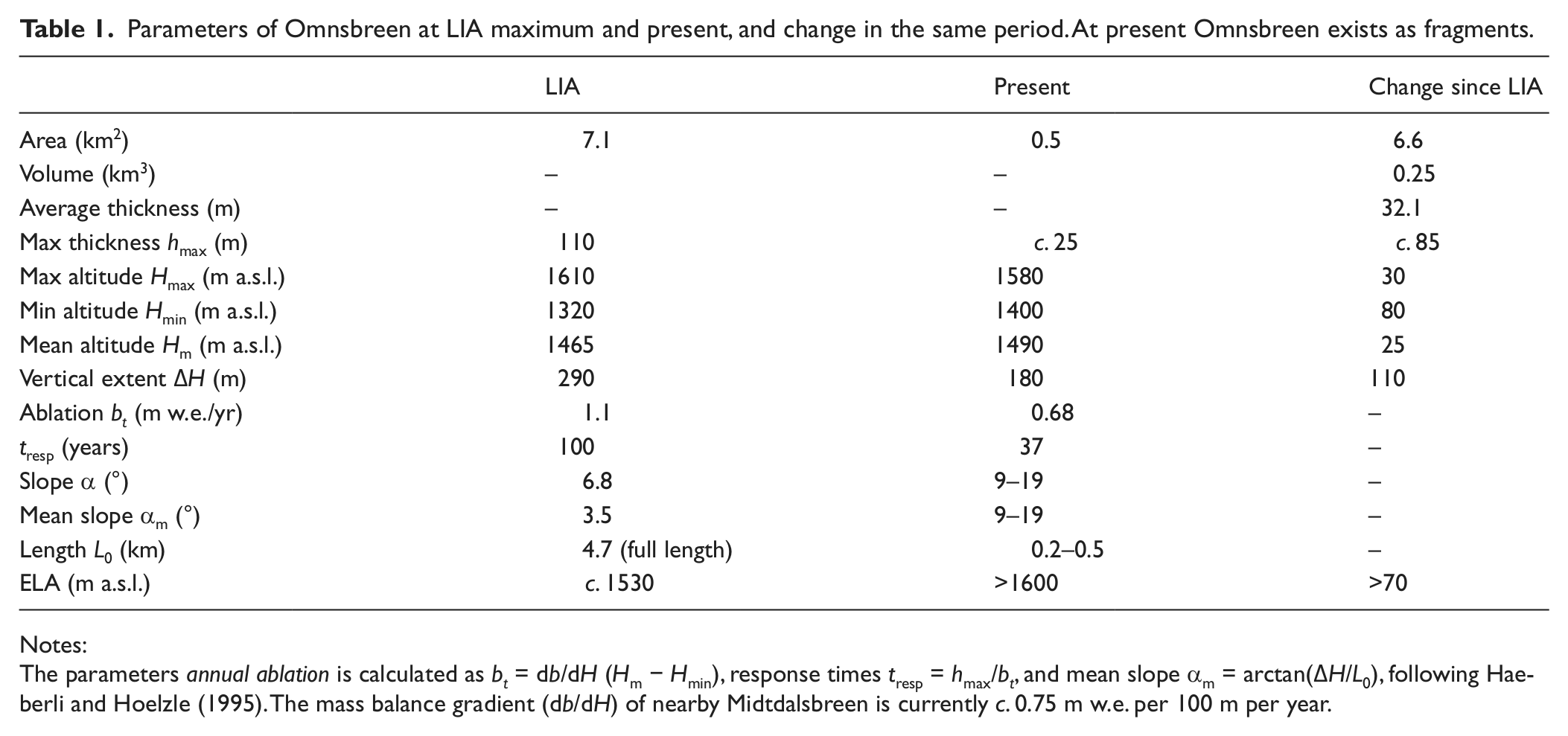
Notes: The parameters annual ablation is calculated as b_t = db/dH (H_m − H_min), response times t_resp = h_max/b_t, and mean slope α_m = arctan(ΔH/L₀), following Haeberli and Hoelzle (1995). The mass balance gradient (db/dH) of nearby Midtdalsbreen is currently c. 0.75 m w.e. per 100 m per year.

Changes of Omnsbreen between the LIA and the present

Comparison of maps from the reconstructed LIA situation with the current (2007) situation makes it possible to quantify glacier changes (Table 1). In total the area of Omnsbreen has been reduced by c. 6.5 km², which is more than 90% of the maximum size during the LIA. In the same period the volume has been reduced by 0.25 km³. Most of the glacier change occurred between 1930 and 1985 (Figure 2), to our knowledge representing a glacier mass loss rate unknown from elsewhere in Norway. Between 1955 and 2007, the glacier decreased spatially from 3 km² to 0.5 km², an area reduction of more than 80%. The glacieret or even ice patches that constitute Omnsbreen at present is a type of accumulation often connected with permafrost areas, based on the assumption that they by definition are thin and the surface temperature does not exceed 0°C (Haeberli, 2000; Nesje et al., 2012). Currently mostly movement by deformation is expected, and the net movement rate considered insignificant.

Stratigraphy and datings

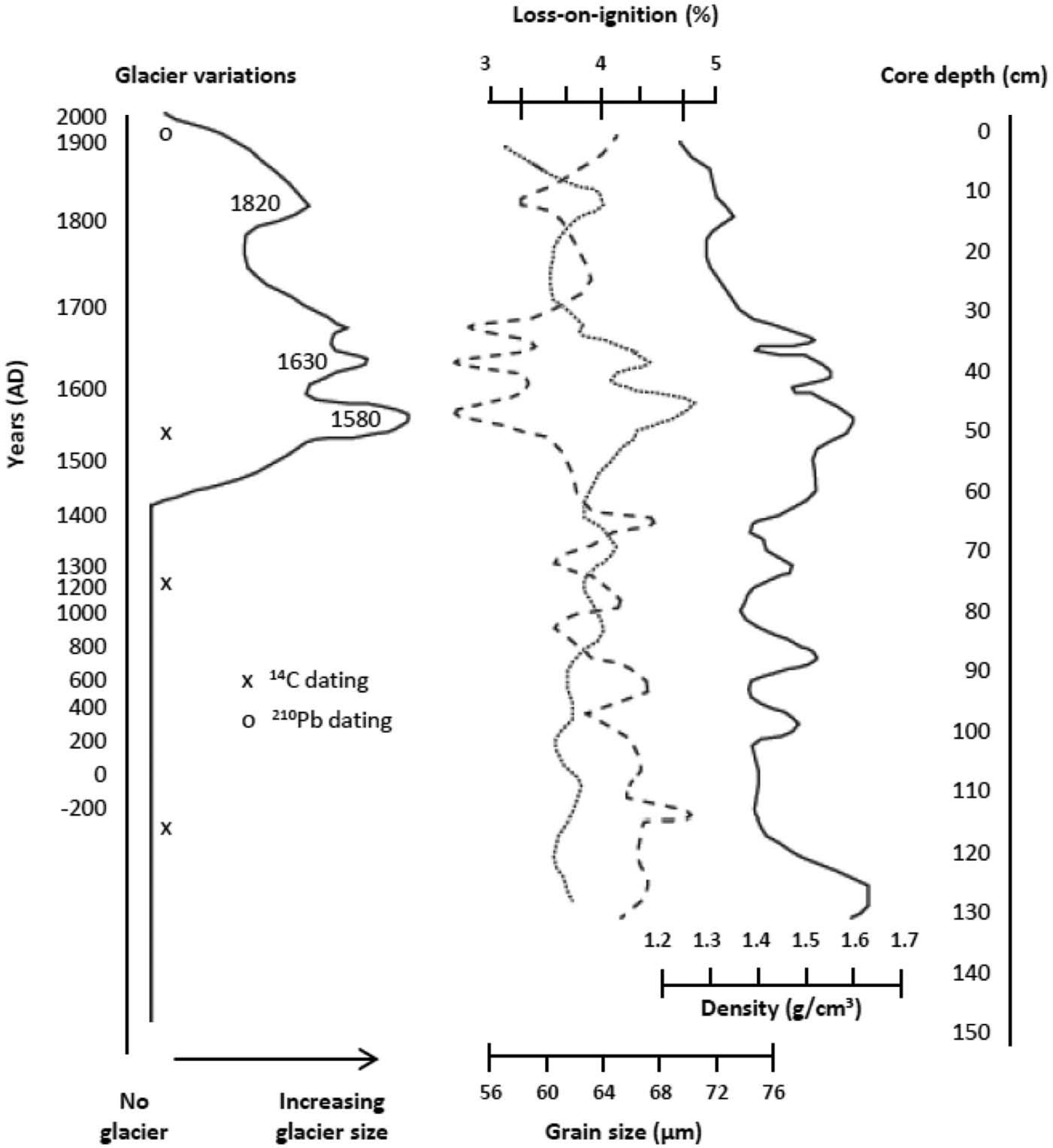
In the lake record a distinct change in the sedimentation rate in Omnsvatnet is observed, from ~0.27 to ~1.47 mm/yr combined with a decrease in the organic content and an increase in the silt content (Figure 9). This event was dated to ad 1425 ± 85 yr and interpreted to represent the formation of Omnsbreen in the lake catchment. This date is in close agreement with radiocarbon-dated terrestrial plant remains that were covered when Omnsbreen was formed, dated at ad 1430 ± 100 yr (Elven, 1978). In addition, based on the analyses of the sediments in Lake Omnsvatnet, Sægrov (2006) inferred significant glacier advances of Omnsbreen around ad 1580, 1630 and 1820, at 47 cm, 38 cm and 12 cm depth, respectively. Based on this we assume an initial LIA glacier formation in the Omnsbreen area during the 15th century, which roughly corresponds to the onset of the LIA period in northern Europe (e.g. Grove, 1988).

Figure 9.

Properties of lacustrine core 2. Interpreted glacial variation is shown at left, grain size (dotted line), loss-on-ignition (dashed line), and sediment density are shown at right. The figure is simplified from Sægrov (2006).

Ground thermal regime and permafrost modelling

At the three sites at Omnsbreen where air temperatures are recorded, the mean temperatures are negative for each of the four full years of measurements, whereas the mean ground surface and ground temperatures at different depths, with one exception, are positive, indicating a positive temperature gradient from the surface into the ground (see Table 2 for all ground temperature characteristics). From these observations, permafrost is not widely expected in the area today. However, at 100 cm depth at site 4 a large year-to-year variation in the period of measurements is observed, from positive temperatures the first years (2007–2010) of measurements to prevailing negative temperatures in 2010–2011 (Figure 10). Observations on snow and meteorology show that the first two years of measurements were characterized by a thick snow cover at site 4, while the last two years both were characterized by low winter temperatures in combination with a shallow snow cover. In 2010 temperatures at site 4 were distinctly lower than the previous years, especially at 100 cm depth, and the temperature during the summer 2011 was never positive. Indeed, an attempt to change a malfunctioning sensor at 50 cm depth in early September 2011 revealed frozen ground at 30 cm depth. The MAAT is presumably too high to allow for widespread permafrost, but discontinuous to more sporadic permafrost patches may exist at this elevation today, especially at wind-exposed sites.

Table 2.

Temperature parameters associated with the four sites of miniature temperature loggers (named 1, 2, 3, and 4 in table).

	1	2	3	4
Elevation (m a.s.l.)	1210	1559	1431	1508
MAAT (°C)	−0.25	−1.65^*	−1.75	–
MAGST (°C)	2.24	−0.49	1.75	0.56^*
MAGT 25 cm (°C)	–	–	–	1.51
MAGT 50 cm (°C)	–	–	–	1.35^*
MAGT 100 cm (°C)	–	–	–	0.97
DDT_a (°C days)	1055	745^*	701	–
DDF_a (°C days)	−1148	−1347^*	−1339	–
DDT_s (°C days)	1037	733	781	538^*
DDF_s (°C days)	−219	−913	−144	−332^*
Frost index (dimensionless)	0.29	0.51	0.26	0.44^*
CryoGRID1.0 (1961–1990) (°C)	0.3	−0.6	0.2	−0.6
CryoGRID1.0 (1981–2010) (°C)	0.6	−0.3	−0.1	−0.3

Notes: All numbers are averaged values for the observation period 2006–2011, while indexed (*) numbers indicate measurements for 2007–2008 only. CryoGRID1.0-values are collected from corresponding cells in the CryoGRID1.0-model, which integrates an area of 1 km².

MAAT: Mean Annual Air Temperature; MAGST: Mean Annual Ground Surface Temperature; MAGT: Mean Annual Ground Temperature; DDT_a: Thawing Degree-Days (air); DDT_s: Thawing Degree-Days (surface); DDF_a: Freezing Degree-Days (air); DDF_s: Freezing Degree-Days (surface); CryoGRID1.0: Temperature at the Top of Permafrost.

Figure 10.

(a) Mean annual temperatures at the surface and three depths in the ground at site 4, the four full years of measurements. For years where holes in the data set exist, the temperatures are linearly interpolated, see Table 2 for details. The very cold 2010 observations stand out in this data set. (b) Complete record of the logger at 100 cm depth, with the varying temperatures indicating snow thickness variations.

The CryoGRID1.0 model indicates that permafrost currently exists at marginal areas of Omnsbreen. Also in adjacent areas such as the margins of Midtdalsbreen and the high-altitude Hallingskarvet, present-day permafrost is reproduced (Gisnås, 2011; Lilleøren et al., 2012), in accordance with observations by Etzelmüller et al. (2003b) and Liestøl and Sollid (1980). The TTOP prediction at site 4 gives a mean ground temperature at −0.5°C for the normal period (1961–1990), and slightly higher temperatures considering the last 30 yr period (1981–2010). At the same time, TTOP predictions at site 1 in the Finse valley change from negative to positive, i.e. from a permafrost situation to a seasonal frost situation (see Table 2). When the CryoGRID1.0 input parameters were altered to reflect LIA conditions, permafrost is widely reproduced in the Finse area in spite of increased snow depths.

Discussion

The temporal constraint of Omnsbreen

The formation of Omnsbreen in the 15th century was considerably later than other Norwegian glaciers (Nesje, 2009), including the adjacent Hardangerjøkulen to the south. There, stratigraphic studies in proglacial terrestrial sites and downstream lakes in the Finse area show that the glacier reformed around 3800 cal. yr BP after having been periodically totally melted away (Dahl and Nesje, 1996). Before the onset of the LIA glacier advance of Blåisen, a northern outlet glacier of Hardangerjøkulen, at approximately ad 1400, the glacier was in advanced position around ad 1050–1100 and ad 1200–1250.

The topographical setting of Omnsbreen makes this glacier sensitive to changes in the North Atlantic Oscillation (NAO), influencing winter precipitation. The times of significant glacier advances of Omnsbreen may indicate a predominantly positive NAO weather mode during the LIA, in close agreement with the evidence presented by Nesje et al. (2007). Mass balance measurements at Rembesdalsskåka, a SW outlet glacier from Hardangerjøkulen located about 15 km SSW of Omnsbreen, show that the net mass balance is related to the NAO index (r² = 0.5).

Development of Omnsbreen

Westerly and southwesterly winds presently reaching the western coast of Norway channels through the fjord branches and, when reaching the high-altitude paleic surface at the end of the fjord, snow will be transported across the plateau, until reaching the valley where Omnsbreen is located. This situation, in combination with the mapped snow cover surface forms and the measured wind directions at Finse, indicates that the topographical location in the landscape makes Omnsbreen an almost ideal example of a glacier nurtured mainly by wind-transported snow. The combination of higher wind velocities and lower temperatures at the onset of the LIA around ad 1400 (Kreutz et al., 1997), led to the formation of Omnsbreen in the western slope of a valley where permafrost was probably under development given the currently very sensitive ground thermal regime (Figure 11). At its maximum LIA position, the geometry of the glacier made accumulation of snow redistributed by wind less efficient, and it is likely that the summit areas of the glacier were subjected to deflation by the westerly winds, thus limiting the glacier from further vertical growth. However, the thickness of the glacier led to temperate basal conditions and talik formation. As the glacier retreated, it once again became possible for wind-redistributed snow to accumulate efficiently in lee areas, and the presently small glacier is probably entirely dependent on this accumulation of wind-transported snow for its continued existence. One cannot rule out the possibility that similar wind- and topography-induced changes between these two semi-stable glacier situations have occurred several times during the Holocene history of Omnsbreen glacier. Also the permafrost is sensitive to the distribution of snow. Thick and stable snow cover early in the season protects the ground from heat loss during winter, while a thin snow cover leads to directly linked ground and air temperatures. Thus, the wind-distributed snow that sustains the presence of Omnsbreen in turn reduces the potential of perennial frozen ground conditions.

Figure 11.

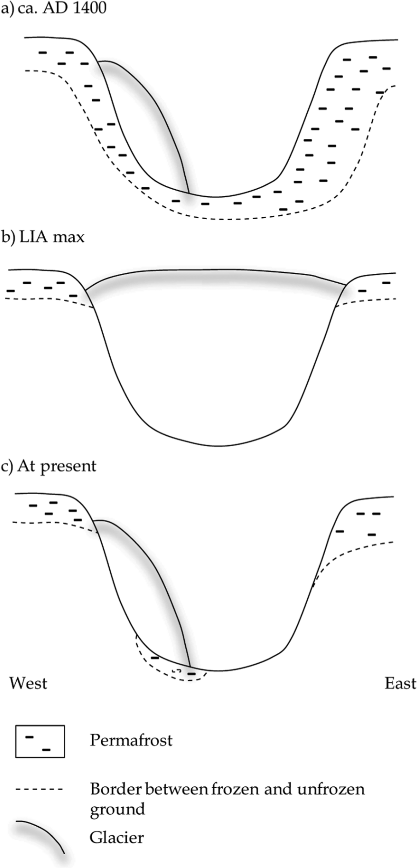
Sketch of Omnsbreen’s development since approximately ad 1400 until present. The varying and asymmetrical permafrost presence is indicated.

The spatial constraint of Omnsbreen

Previous mapping of the glacier’s maximum extent during the LIA suggested an area of 12–14 km² (Elven, 1978). This study, however, probably included perennial firn and snow patches and combined these with other glaciers further northwest, which, according to the present study, was not dynamically connected to Omnsbreen during the LIA. The present study suggests a maximum area of Omnsbreen of around 7.1 km² (Figure 5). Interestingly, by calculating the area of Omnsbreen as interpreted from maps drawn in 1927 the result is 5.8 km² (Elven, 1978) or 6.8 km² (Liestøl and Sollid, 1980). If this is correct, the bulk of the glacier disappeared during a period of only 55 years, from 1930 to 1985, until it reached its current size of less than 0.5 km². In the same period, the total glacier area in Jotunheimen was reduced by 23%, with an area loss of up to 60% for a few individual glaciers (Andreassen et al., 2008). To our knowledge, the rate of mass loss observed at Omnsbreen is unparalleled in observations elsewhere.

Lack of glacier marginal landforms indicative of an active glacier terminus such as terminal moraines can be due to at least four different and mutually inclusive explanations; (1) lack of surrounding headwalls where extra-glacial debris input could be formed, which is a common feature where glaciers e.g. form large, and sometimes ice-cored moraines (see e.g. Zemp et al., 2005), (2) little erosion of the substrata, and as a consequence little mobilization of debris available for moraine formation, (3) gradual transition from a dynamically active glacier to non-active perennial firn- and ice-fields, and (4) low landforming potential because of cold glacier margins terminating in a permafrost environment. Explanations (1), (3) and (4) are all plausible in this area, whereas explanation (2) does not seem valid. Below the central parts of the former glacier and in the areas with maximum shear stress landforms and sediment cover rather indicate that the subglacial activity has been high. Explanation (4) is supported by our CryoGRID1.0 results of the LIA, independent of glacier presence.

Both the calculated deformation velocity and shear stress of the maximum LIA Omnsbreen are low, and reflect the limited thickness over large parts of the glacier. However, the values are comparable with those of small polythermal glaciers in Spitsbergen (Longyearbreen and Larsbreen; Etzelmüller et al., 2000). The basal sliding was not considered here, but the large assemblage of subglacial landforms suggests considerable basal movement. The distribution of striae and flutes largely corresponds to areas of maximum deformation velocity and shear stresses, while the distribution of ‘domino’-structures seems partly associated with transition areas between high and low glacier activity. The glaciers response time was estimated to 100 years, however based on a modern mass balance gradient. Compared with glacier inventories of the present-day European Alps, the LIA Omnsbreen fits well into the parameter schemes provided in e.g. Haeberli and Hoelzle (1995).

Climate, glaciers and permafrost duringthe ‘Little Ice Age’

During the LIA, the northwestern areas of Europe cooled to a larger degree than central Europe, and an increased temperature gradient between the two regions developed (Bradley and Jones, 1993). As a result of this enhanced temperature gradient the cyclonic activity increased, especially resulting in intense winter storms of strengths that are not recorded since 1850 (Lamb, 1979). The concentration of sodium ions (Na⁺) in Greenland ice core records (GISP2) is commonly used as proxy data for the intensity and frequency of storm activity in the north Atlantic, when salt from seawater is deposited on the Greenland ice sheet (Dawson et al., 2007). From c. ad 1400 the Na⁺ concentration in this record increases by 20–30% over a period of only 20 years, which corresponds to the onset of the LIA (Fischer et al., 1998; Kreutz et al., 1997). Within the LIA this record shows significant variability at decadal scales, but is particularly high from 1680 to 1730. This period also corresponds to a minimum stage in the general low solar activity during the LIA (Mauquoy et al., 2002). Thus, during the LIA several observations and records of increased storm activity in the north Atlantic region exist, and in Norway these storms are likely to have reached land from west or southwest, not unlike the present situation, however enhanced. The implications of enhanced storm frequency especially during winter are twofold: (1) precipitation as snow will increase and (2) higher potential of snow redistribution by wind. In high-mountain areas where snow has the potential to survive summers, many perennial snow patches probably built up in this way during the LIA. Perennial snow-patches in areas that today are snow free in summer are known from for example the Cairngorm Mountains in Scotland during the LIA (Lamb, 1979). It is likely that the situation in Norway was similar to that in Scotland; many perennial snow or ice patches must have built up in areas that are today snow free. In this climatic setting Omnsbreen stands out as an example of one of these initially perennial ice patches formed in a lee position that eventually grew into a glacier.

From modelling of the ground thermal regime (Gisnås et al., 2013; Lilleøren et al., 2012) we conclude that permafrost has played a major role in the Holocene landscape development, and during the LIA much larger areas than at present were underlain by permafrost. In this respect, the Omnsbreen area represents the lowermost and westernmost area that was affected by permafrost during the LIA in Scandinavia, in areas that seemingly were permafrost free since the regional deglaciation. Owing to limitations on growth by the local topography, thin glacier marginal zones are expected and also modelled based on the interpreted LIA size of the glacier, and cold glacier margins were likely to form. The sediment availability and glacier dynamics are decisive of what kind of marginal landforms that can develop under such conditions, and both ice-cored moraines and moraine-derived rock glaciers need a high amount of material added to the glacier surface and most often occur where a weathering headwall is present above the glacier. Omnsbreen more or less filled its valley entirely, and no such external sediment source was then available. There has, however, been partly high subglacial activity and in many places in the glacier marginal zone thick sediment cover is present. Shearing processes bringing material to the glacier surface are expected in such an environment and these processes alone do not necessarily produce pronounced moraine ridges. In the Omnsbreen case a cold glacier margin is likely seen in the light of our interpretations of the ‘domino’-structures. Since the ‘domino’-structures are site-specific landforms, it is not easy to directly relate the suite of landforms present at Omnsbreen to other regions, but we still suggest that the mere lack of glacier-marginal landforms encompassing the former glacierized zone, in combination with recent regional permafrost modelling of the LIA, might provide a tool to recognize former cold or polythermal glaciers. Further, observations from Norway and Iceland show that in maritime permafrost environments, the most frequently occurring type of permafrost landforms are those formed in connection with glacial activity, such as moraine-derived rock glaciers and ice-cored moraines (Lilleøren and Etzelmüller, 2011). The geomorphic potential of interacting processes between glaciers and permafrost is significant, and the acknowledgement of glacier–permafrost systems as important landscape elements, and not just as individual processes, will increase the understanding of the development and processes involved in a cryo-conditioned landscape.

Conclusions

Since the ‘Little Ice Age’ Omnsbreen has been reduced by an area of 6.5 km² (90%) and a volume of 0.25 km³, with most of the reduction occurring between ad 1930 and 1985. The observed retreat rate is greater than any other known glacier retreat rates in Norway at the same period.

Analyses and dating of lake sediments from Omnsvatnet indicate an initial ‘Little Ice Age’ formation of Omnsbreen at ad 1425 ± 85, thus a later formation than the main glacier reappearance in Norway, mainly occurring as Neoglaciation phenomena in Norway from c. 6000 to 5000 yr BP. Studies of the lake sediments in Omnsvatnet indicate that Omnsbreen was in advanced positions around ad 1580, 1630 and 1820.

The topographical setting of Omnsbreen, situated along the east-facing slope of a north–south trending valley, makes the glacier sensitive to changes in the prevailing westerly winds for mass accumulation. Both glacier and permafrost exist as marginal phenomena in the Omnsbreen area. While the glaciers depend on lee side accumulation of snow, the permafrost is sensitive to snow deflation causing heat loss from the ground during winter. This observation confirms the mutual exclusive nature of permafrost and glacier presence in marginal zones of either phenomenon.

The lack of terminal moraine systems and the modelled occurrence of permafrost suggest that Omnsbreen had cold margins during the LIA when it terminated in a permafrost environment. Here, we hypothesize that ice-cored moraines, moraine-derived rock glaciers and push moraines may not be the only results of such interaction. Instead, we propose that also the lack of clear marginal landforms like observed at Omnsbreen can be indicative of cold glacier margins.

Footnotes

Acknowledgements

The authors extend their thanks to the Department of Geosciences, University of Oslo and the Alpine Research Centre at Finse. Sægrov kindly provided data from the lacustrine sediment cores used in his MSc thesis, and Dr Kirsty Langley gave helpful comments and advice during the writing process. This is publication no. A398 from the Bjerknes Centre for Climate Research.

Funding

The fieldwork was carried out as a part of the MSc thesis of KS Lilleøren funded by the Department of Geosciences, University of Oslo, and was made possible through the use of the Alpine Research Centre at Finse.

References

Alley

Gow

Johnson

. (1995) Comparison of deep ice cores. Nature 373: 393–394.

Andreassen

Elvehøy

Jackson

. (2010) Glaciological investigations in Norway in 2009. In: Kjøllmoen

(ed.) Report No. 2. Oslo: Norwegian Water Resources and Energy Directorate.

Andreassen

Elvehøy

Kjøllmoen

. (2005) Glacier mass-balance and length variation in Norway. Annals of Glaciology 42: 317–325.

Andreassen

Paul

Kääb

. (2008) Landsat-derived glacier inventory for Jotunheimen, Norway, and deduced glacier changes since the 1930s. The Cryosphere 2: 131–145.

Bamber

Payne

(2004) Mass Balance of the Cryosphere. Cambridge University Press.

Benn

Evans

DJA

(1998) Glaciers and Glaciation. London: Arnold, 734 pp.

Berthling

Etzelmüller

(2011) The concept of cryo-conditioning in landscape evolution. Quaternary Research 75: 378–384.

Björnsson

Gjessing

Hamran

S-E

. (1996) The thermal regime of sub-polar glaciers mapped by multi-frequency radio-echo sounding. Journal of Glaciology 42: 23–32.

Bjune

Birks

HJB

Seppa

(2004) Holocene vegetation and climate history on a continental–oceanic transect in northern Fennoscandia based on pollen and plant macrofossils. Boreas 33: 211–223.

10.

Bradley

Jones

(1993) ‘Little Ice Age’ summer temperature variations: Their nature and relevance to recent global warming trends. The Holocene 3: 367–376.

11.

Brohan

Kennedy

Harris

. (2006) Uncertainty estimates in regional and global observed temperature changes: A new data set from 1850. Journal of Geophysical Research 111: D12106.

12.

Cogley

Hock

Rasmussen

. (2011) Glossary of Glacier Mass Balance and Related Terms. HP-VII Technical Documents in Hydrology No. 86, IACS Contribution No. 2, Paris: UNESCO-IHP.

13.

Dahl

Nesje

(1996) A new approach to calculating Holocene winter precipitation by combining glacier equilibrium-line altitudes and pine-tree limits: A case study from Hardangerjøkulen, central southern Norway. The Holocene 6: 381–398.

14.

Dawson

Hickey

Mayewski

. (2007) Greenland (GISP2) ice core and historical indicators of complex North Atlantic climate changes during the fourteenth century. The Holocene 17: 427–434.

15.

DNMI (2007) E-Klima. Norwegian Meteorological Office. Last accessed July 2006 from: http://shimmer.oslo.dnmi.no/portal/page?_pageid=35,96278,35_96303&_dad=portal&_schema=PORTAL.

16.

Dyurgerov

(2003) Mountain and subpolar glaciers show an increase in sensitivity to climate warming and intensification of the water cycle. Journal of Hydrology 282: 164–176.

17.

Elven

(1978) Subglacial plant remains from the Omnsbreen glacier area, south Norway. Boreas 7: 83–89.

18.

Etzelmüller

Björnsson

(2000) Map analysis techniques for glaciological applications. International Journal of Geographical Information Science 14: 567–581.

19.

Etzelmüller

Hagen

J-O

(2005) Glacier-permafrost interaction in arctic and alpine mountain environments with examples from Southern Norway and Svalbard. In: Harris

Murton

(eds) Cryospheric Systems: Glaciers and Permafrost. Geological Society, London, Special Publications, pp. 11–27.

20.

Etzelmüller

Berthling

Ødegård

(2003a) 1D-DC-resistivity depth soundings in high mountain areas of Southern Norway – A tool in permafrost investigations. Zeitschrift für Geomorphologie 132: 19–36.

21.

Etzelmüller

Berthling

Sollid

(2003b) Aspects and concepts on the geomorphological significance of Holocene permafrost in Southern Norway. Geomorphology 52: 87–104.

22.

Etzelmüller

Hoelzle

Heggem

ESF

. (2001) Mapping and modelling the occurence and distribution of mountain permafrost. Norsk geografisk tidsskrift – Norwegian Journal of Geography 55: 186–194.

23.

Etzelmüller

Ødegård

Vatne

. (2000) Glacier characteristics and sediment transfer system of Longyearbreen and Larsbreen, western Spitsbergen. Norsk geografisk tidsskrift – Norwegian Journal of Geography 55: 157–168.

24.

Fischer

Werner

Wagenbach

. (1998) Little ice age clearly recorded in Northern Greenland ice cores. Geophysical Research Letters 25: 1749–1752.

25.

Gisnås

(2011) Modelling of permafrost in Norway using two equilibrium models. MSc Thesis, Department of Geosciences, University of Oslo. Available at http://www.duo.uio.no/publ/geofag/2011/134415/Permafrost_distribution_in_Norway.pdf

26.

Gisnås

Etzelmüller

Farbrot

. (2013) CryoGRID 1.0 – Permafrost distribution in Norway estimated by a spatial numerical model. Permafrost and Periglacial Processes DOI: 10.1002/ppp.1765.

27.

Glen

(1955) The creep of polycrystalline ice. Proceedings of the Royal Society of London. Series A. Mathematical and Physical Sciences 228: 519–538.

28.

Grove

(1988) The Little Ice Age. London: Methuen.

29.

Haeberli

(2000) Modern research perspectives relating to permafrost creep and rock glaciers. Permafrost and Periglacial Processes 11: 290–293.

30.

Haeberli

(2005) Investigating glacier–permafrost relationships in high-mountain areas: Historical background, selected examples and research needs. In: Harris

Murton

(eds) Cryospheric Systems: Glaciers and Permafrost. The Geological Society of London, Special Publication 242, pp. 29–37.

31.

Haeberli

Burn

(2002) Natural hazards in forests: Glacier and permafrost effects as related to climate change. In: Sidle

(ed.) Environmental Change and Hazards in Forests. Wallingford/New York: CABI, pp. 167–202.

32.

Haeberli

Hoelzle

(1995) Application of inventory data for estimating characteristics of and regional climate-change effects on mountain glaciers: A pilot study with the European Alps. Annals of Glaciology 21: 206–212.

33.

Haeberli

Noetzli

Zemp

. (2005) Glacier Mass Balance Bulletin. IUGG – UNEP – UNESCO – WMO, Compiled by the World Glacier Monitoring Service (WGMS).

34.

Harris

Corte

(1992) Interactions and relations between mountain permafrost, glaciers, snow and water. Permafrost and Periglacial Processes 3: 103–110.

35.

Harris

Murton

(2005) Interactions between glaciers and permafrost: An introduction. In: Harris

Murton

(eds) Cryospheric Systems: Glaciers and Permafrost. The Geological Society of London, Special Publication 242, pp. 1–9.

36.

Hock

(2005) Glacier melt: A review of processes and their modelling. Progress in Physical Geography 29: 362–391.

37.

Hutchinson

(1989) A new procedure for gridding elevation and stream line data with automatic removal of spurious pits. Journal of Hydrology 106: 211–232.

38.

Hutchinson

Dowling

(1991) A continental hydrological assessment of a new grid-based digital elevation model of Australia. Hydrological Processes 5: 45–58.

39.

Høgvard

(1987) Omnsbreen. Dannelse og avsmelting. Hovedoppgave i naturgeografi (M.Sc.thesis), University of Oslo (in Norwegian).

40.

King

(1986) Zonation and ecology of high-mountain permafrost in Scandinavia. Geografiska Annaler – Series A Physical Geography 68: 131–139.

41.

Kleman

Borgström

(1994) Glacial landforms indicative of a partly frozen bed. Journal of Glaciology 40: 255–264.

42.

Kleman

Hättestrand

(1999) Frozen-bed Fennoscandian and Laurentide ice sheets during the last glacial maximum. Nature 402: 63–66.

43.

Kreutz

Mayewski

Meeker

. (1997) Bipolar changes in atmospheric circulation during the Little Ice Age. Science 277: 1294–1296.

44.

Lamb

(1979) Climatic variation and changes in the wind and ocean circulation: The Little Ice Age in the northeast Atlantic. Quaternary Research 11: 1–20.

45.

Lauritzen

Lundberg

(1999) Calibration of the speleothem delta function: An absolute temperature record for the Holocene in northern Norway. The Holocene 9: 659–669.

46.

Liestøl

(1977) Pingos, springs and permafrost in Spitsbergen. Norsk polarinstitutts Aarbok (1975), pp. 7–30.

47.

Liestøl

(2000) Glaciology. Perspektiv. Department of Physical Geography, University of Oslo, Oslo, 123 pp.

48.

Liestøl

Sollid

(1980) Glacier erosion and sedimentation at Hardangerjøkulen and Omnsbreen. In: Orheim

(ed.) Field Guide to Excursion Organized in Conjunction with Symposium on Processes of Glacier Erosion and Sedimentation. Geilo, 25–30 August 1980. Norwegian Polar Institute.

49.

Lilleøren

Etzelmüller

(2011) A regional inventory of rock glaciers and ice-cored moraines in Norway. Geografiska Annaler Series A – Physical Geography 93: 175–191.

50.

Lilleøren

Etzelmüller

Gisnås

. (2012) The relative age of mountain permafrost – estimation of Holocene permafrost limits in Norway. Global and Planetary Change DOI: 10.1016/j.gloplacha.2012.05.016.

51.

Matthews

Berrisford

Dresser

. (2005) Holocene glacier history of Bjornbreen and climatic reconstruction in Central Jotunheimen, Norway, based on proximal glaciofluvial stream-bank mires. Quaternary Science Reviews 24: 67–90.

52.

Mauquoy

Van Geel

Blaauw

. (2002) Evidence from northwest European bogs shows ‘Little Ice Age’ climatic changes driven by variations in solar activity. The Holocene 12: 1–6.

53.

Messel

(1971) Mass and Heat Balance of Omnsbreen – A Climatically Dead Glacier in Southern Norway. Oslo: Norwegian Polar Institute: Skrifter.

54.

Nesje

(1992) A piston corer for lacustrine and marine sediments. Arctic and Alpine Research 24: 257–259.

55.

Nesje

(2009) Latest Pleistocene and Holocene alpine glacier fluctuations in Scandinavia. Quaternary Science Reviews 28: 2119–2136.

56.

Nesje

Matthews

(2012) The Briksdalsbre Event: A winter precipitation-induced decadal-scale glacial advance in southern Norway in the ad 1990s and its implications. The Holocene DOI: 10.1177/0959683611414938.

57.

Nesje

Bakke

Dahl

. (2008) Norwegian mountain glaciers in the past, present and future. Global and Planetary Change 60: 10–27.

58.

Nesje

Dahl

Thun

. (2007) The ‘Little Ice Age’ glacial expansion in Western Scandinavia: Summer temperature or winter precipitation? Climate Dynamics 30: 789–801.

59.

Nesje

Jansen

Birks

. (2005) Holocene climate variability in the Northern north Atlantic region: A review of terrestrial and marine evidence. Geophysical Monograph Series 158: 289–322.

60.

Nesje

Lie

Dahl

(2000) Is the North-Atlantic Oscillation reflected in Scandinavian glacier mass balance records? Journal of Quarternary Science 15: 587–601.

61.

Nesje

Matthews

Dahl

. (2001) Holocene glacier fluctuations of Flatebreen and winter-precipitation changes in the Jostedalsbreen region, Western Norway, based on glaciolacustrine sediment records. The Holocene 11: 267–280.

62.

Nesje

Pilø

Finstad

. (2012) The climatic significance of artefacts related to prehistoric reindeer hunting exposed at melting ice patches in southern Norway. The Holocene 22: 485–496.

63.

Nye

(1965) The flow of a glacier in a channel of rectangular, elliptic or parabolic cross-section. Journal of Glaciology 5: 661–690.

64.

O’Brien

Mayewski

Meeker

. (1995) Complexity of Holocene climate as reconstructed from a Greenland ice core. Science 270: 1962–1964.

65.

Paterson

WSB

(1994) The Physics of Glaciers. Oxford: Pergamon/Elsevier Science, 480 pp.

66.

Phillips

Hall

Mottram

. (2006) Cosmogenic ¹⁰Be and ²⁶Al exposure ages of tors and erratics, Cairngorm Mountains, Scotland: Timescales for the development of a classic landscape of selective linear glacial erosion. Geomorphology 73: 222–245.

67.

Renberg

(1991) The HOH-Kajak sediment corer. Journal of Paleolimnology 6: 167–170.

68.

Sægrov

(2006) Rekonstruksjon av Omnsbreen gjennom holosen basert på terrestriske studier og proglasiale kjerner. MSc Thesis, Department of Earth Science, University of Bergen (in Norwegian).

69.

SeNorge (2011) Normal Annual Maximum Snow Amount (1971–2000) NVE, Met.no, The Norwegian Mapping Authorities. Accessed 1 October 2011 from: http://senorge.no/mappage.aspx

70.

Shumskii

(1964) Principles of Structural Glaciology. New York: Dover Publications, Inc., 497 pp.

71.

Sigmond

EMO

Askvik

(2008) Hardangerjøkulen: 1416 II : Berggrunnskart. Trondheim: Norwegian Geological Survey.

72.

Smith

Riseborough

(1996) Permafrost monitoring and detection of climate change. Permafrost and Periglacial Processes 7: 301–309.

73.

Smith

Riseborough

(2002) Climate and the limits of permafrost: A zonal analysis. Permafrost and Periglacial Processes 13: 1–15.

74.

Sollid

Sørbel

(1988) Influence of temperature conditions in formation of end moraines in Fennoscandia and Svalbard. Boreas 17: 553–558.

75.

Sollid

Sørbel

(1994) Distribution of glacial landforms in Southern Norway in relation to the thermal regime of the last continental ice sheet. Geografiska Annaler 76A: 25–36.

76.

Zemp

Kääb

Hoelzle

. (2005) GIS-based modelling of the glacial sediment balance. Zeitschrift Für Geomorphologie 138: 113–129.

Holocene development and geomorphic processes at Omnsbreen,southern Norway: Evidence for glacier–permafrost interactions

Abstract

Keywords

Introduction

Study area

Methods

Climate data analysis

Geomorphological mapping

Reconstruction of the glacier geometry and associated parameters

Lake sediment cores from Omnsvatnet

Modelling of ground thermal regime

Results

Observations on temperature, lapse rates, wind and snow cover

Glacial geomorphology at Omnsbreen

Reconstruction of LIA glacier geometry and extent

Changes of Omnsbreen between the LIA and the present

Stratigraphy and datings

Ground thermal regime and permafrost modelling

Discussion

The temporal constraint of Omnsbreen

Development of Omnsbreen

The spatial constraint of Omnsbreen

Climate, glaciers and permafrost duringthe ‘Little Ice Age’

Conclusions

Footnotes

Acknowledgements

Funding

References