Stacking of discontinuous regional palaeoclimate records: Chironomid-based summer temperatures from the Alpine region

Stacking and splicing procedure

The stacking procedure presented here consists of several steps, including (1) altitudinal correction of temperatures (necessary in mountainous landscapes), (2) interpolation of the records to equal time intervals, and (3) averaging of values for individual sections of the time interval of interest for which the same number of records are available (the ‘stacking’ in a strict sense). If there are records involved in the stacking procedure that are not continuous over the time window of interest, steps 1–3 above will lead to a number of stacked records, each consisting of averages of a different selection of the available temperature reconstructions. Since individual stacks may be strongly influenced by sites with extreme values, for example, consistently cooler temperatures because of shading or warmer temperatures because of southerly aspect, a further step is necessary to combine the different stacked interval into a continuous temperature record. In this step 4, here referred to as splicing, absolute temperatures in individual stacks are corrected based on overlapping sequences with younger or older stacked records. One of the stacked sequences will have to be identified as the most reliable sequence to which all other stacks are spliced. This ‘anchoring’ of the stack will not influence the overall temporal trends or amplitudes of variation of the stacked sequence but only its absolute values. In the examples provided in this study, we use the stacked segment based on the largest number of records as the anchoring section. If the reconstruction includes the most recent past, anchoring can alternatively also be based on modern, instrumental temperature estimates for the different sites.

Interpolation

Interpolation of values to identical time intervals is accomplished either using linear interpolation or nearest neighbour interpolation. Linear interpolation assigns values based on the closest younger datapoint and the closest older datapoint in a time series. Interpolated values are then calculated as

T i = T y + ( A i − A y ) × ( T o − T y ) / ( A o − A y )

(1)

where T_i is the temperature of the interpolated datapoint, T_y is the temperature of the younger datapoint, T_o the temperature of the older datapoint, A_y the age of the younger datapoint, A_o the age of the older datapoint and A_i the age of the datapoint to be interpolated.

Nearest neighbour interpolation assigns to each interpolated age the same temperature value as associated with the datapoint closest in age in the time series. The examples and simulations presented in this study are interpolated to 20-year intervals.

Simulations of stacked records

To examine how the number of records to be stacked and the choice of interpolation method influence the stacked reconstructions, we simulated palaeoclimate records of 100- to 400-year sampling resolution using the NGRIP δ¹⁸O record on the GICC05 age scale (Rasmussen et al., 2006; Vinther et al., 2006) with 20-year sampling intervals and expressed as years before ad 2000 (b2k). This dataset is one of the most widely used late Quaternary climate proxy records, and since it includes both low frequency, millennial-scale climate variations and abrupt short scale changes, it provides an opportunity to examine how stacking affects the reconstructed climatic signal. Prominent features of the record include the abrupt increase in δ¹⁸O at ~14,700 b2k (the Greenland Stadial (GS)-2 to Greenland Interstadial (GI)-1 transition); the gradual decrease in δ¹⁸O during GI-1 between ~14,400 and ~12,800 b2k, interrupted by short-lived minima at ~14,000, ~13,600 and ~13,100 b2k; the pronounced minimum during GS-1 ~12,800 to ~11,800 b2k; the abrupt increase in δ¹⁸O at the transition to the Holocene ~11,700 b2k; the gradual rise in δ¹⁸O during the early Holocene between ~11,500 and 9500 b2k; and the short-lived minimum during the 8.2 kyr event at ~8200 b2k (Figure 1a). Over the time interval 20–15,000 b2k, the record was subsampled at three different temporal resolutions by randomly calculating time intervals with a mean of 100, 200 and 400 years and a standard deviation of 20, 40 and 80 years, respectively. Although many palaeoclimate records based on lake sediments are available at higher resolution (see, for example, Table 1), records with 100- to 200-year intervals are regularly reported for the Lateglacial period and the early and mid-Holocene. In our simulations, the first randomly calculated interval provided the age for the first (youngest) sample of the simulated dataset, the sum of the first two intervals the age for the second sample, the sum of the first three intervals the age of the third sample and so forth until the maximum age of the simulated dataset exceeded 15,000 years. To each sample, the δ¹⁸O value in the NGRIP record with the most similar age was assigned, resulting in a simulated dataset of randomly selected samples of the NGRIP record spaced at irregular intervals of approximately 100, 200 and 400 years. For stacking, samples were interpolated to evenly spaced 20-year intervals, the same intervals as in the NGRIP δ¹⁸O record, using the procedures of nearest neighbour and linear interpolation outlined above. Several of these randomly produced records were then stacked to examine the extent to which this approach can capture millennial- to centennial-scale variability in the original δ¹⁸O record.

OPEN IN VIEWER

Figure 1.

(a) The Greenland NGRIP δ¹⁸O record used for the simulation experiments (Rasmussen et al., 2006; Vinther et al., 2006). Climatic events discussed in this study are labelled according to Blockley et al. (2012). (b) Examples of two simulated δ¹⁸O records with a mean sampling resolution of 400 years. The records are interpolated using nearest neighbour interpolation. (c) As (b) but with linear interpolation. (d) Stacked records based on four simulated records with a mean sampling interval of 400 years. Stacks were calculated using linear (lin) and nearest neighbour interpolation (nn) and are compared with the original NGRIP δ¹⁸O record.

OPEN IN VIEWER

Table 1.

Geographical and chronological background information on the chironomid records used in this publication, together with the ranges of reconstructed July air temperatures and sample-specific estimated standard errors of prediction for each record. The age estimate of the first evidence for local human impact is also indicated.

Site	Latitude (N)	Longitude (E)	Elevation (m.a.s.l)	Chironomid-inferred July air T (°C)	eSEP (°C)	Oldest reliable date (cal. BP)	Youngest reliable date (cal. BP)	Sample interval for stacking (cal. BP)	Dated horizons (excluding outliers)	Samples in dated age range	Average sample interval	Earliest local human impact (cal. BP)
Hinterburgsee (HIN)	46°43′	8°04′	1515	8.4–13.0	1.36–1.43	11,630 (pollen)	−47 (surface)	810–12130	14	54	215	800
Stazersee (STA)	46°29′	9°52′	1809	8.6–13.8	1.37–1.58	10,596 (C-14)	−51 (surface)	2440–10,690	18	93	114	2440
Foppe (FOP)	46°28′	8°48′	1470	9.6–15.1	1.36–1.57	15,132 (C-14)	9958 (C-14)	10,860–14,920	11	47	110	NA
Maloja Riegel (MAL)	46°24′	9°41′	1865	8.6–13.0	1.51–1.56	13,528 (C-14)	10,854 (C-14)	10,860–13,830	8	54	50	NA
Lac Lautrey (LAU)	46°35′	5°51′	788	11.9–17.7	1.54–1.60	14,640 (pollen)	11,417 (C-14)	11,350–14,920	11	127	25	NA
Lac Anterne (ANT)	45°59′	6°47′	2060	7.3–10.6	1.40–1.57	1750 (layer counting)	−51 (surface)	90–1890	NA	50	36	90

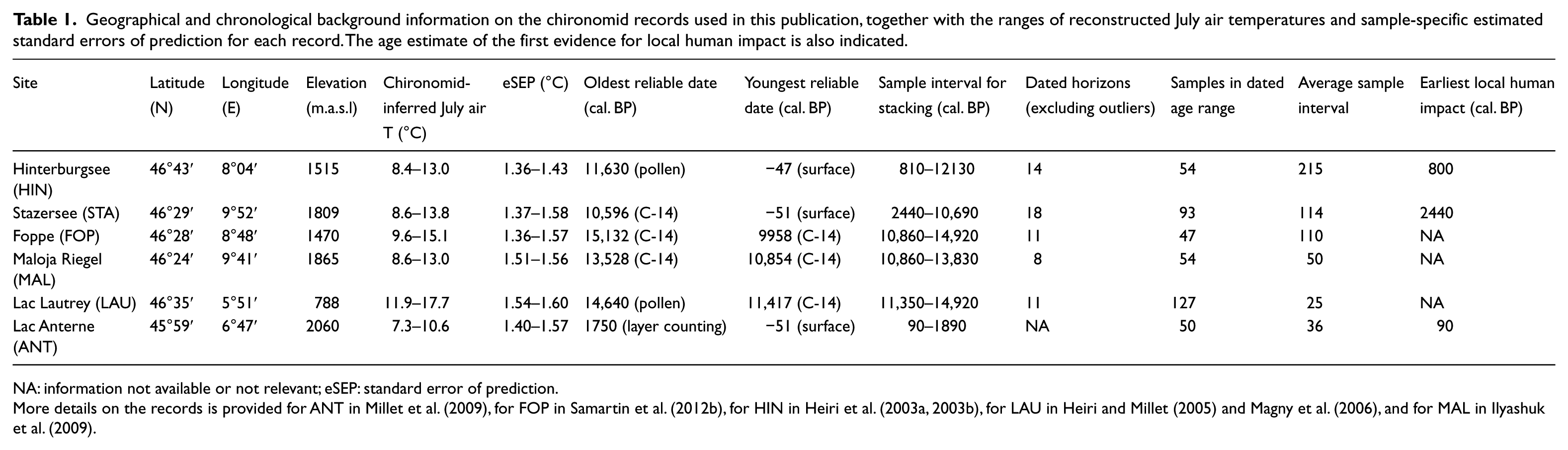
NA: information not available or not relevant; eSEP: standard error of prediction.

More details on the records is provided for ANT in Millet et al. (2009), for FOP in Samartin et al. (2012b), for HIN in Heiri et al. (2003a, 2003b), for LAU in Heiri and Millet (2005) and Magny et al. (2006), and for MAL in Ilyashuk et al. (2009).

Simulation of stacked datasets: Nearest neighbour or linear interpolation?

Examples provided in Figure 1b and c indicate that even at the coarse ~400-year resolution, the simulated datasets capture millennial-scale variability in the δ¹⁸O record relatively well, and that linear and nearest neighbour interpolation seem to be similarly successful at approximating low amplitude variations. During phases of abrupt climatic change, individual simulations are less representative. The extent to which prominent decadal- to centennial-scale features, such as the warming during the earliest GI-1 or the short-lived cooling episodes during this interstadial, are captured by the simulations is strongly influenced by the placement of the selected samples during these intervals (Figure 1b and c). Even if based on only four individual records, stacked reconstructions produced using nearest neighbour and linear interpolation yield almost identical results for the Holocene, for which the δ¹⁸O record, with the exception of the 8.2 kyr event, was mainly characterized by low frequency variations (Figure 1d). Again, both methods performed less well during episodes of rapid climatic transitions. To examine in more detail how the different interpolation methods perform in capturing the abrupt δ¹⁸O variations 15,000–11,000 b2k, we calculated stacks based on two, three and four interpolated records each, using linear and nearest neighbour interpolation and based on ~400- and ~200-year sampling intervals (Figure 2).

OPEN IN VIEWER

Figure 2.

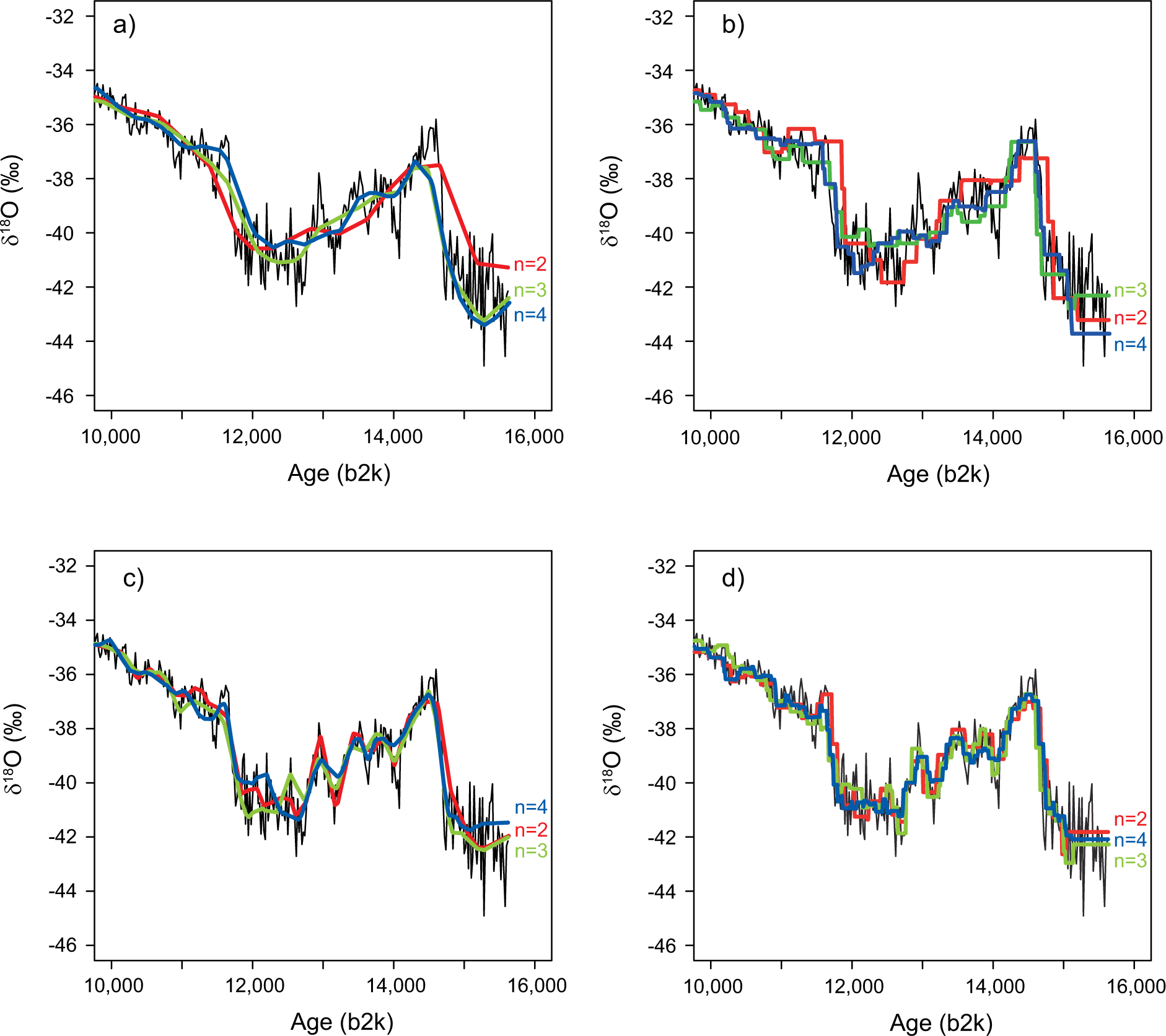
The NGRIP δ¹⁸O record 10,000–15,000 b2k compared with stacked records based on two, three and four simulated records (n = 2–4) with (a and b) 400-year sampling intervals and (c and d) 200-year sampling intervals. Stacks in (a) and (c) are based on linear interpolation and in (b) and (d) on nearest neighbour interpolation.

The two interpolation methods deal differently with abrupt changes between two datapoints. Nearest neighbour interpolation prescribes an abrupt shift in the interpolated values at the mid-point between two datapoints, whereas linear interpolation prescribes a gradual change from one point to the next. We therefore expected nearest neighbour interpolation to be more successful at capturing abrupt shifts in climatic conditions. As expected, linear interpolation resulted in relatively smooth variations in δ¹⁸O even if based on only two stacked records (Figure 2a and c). If additional records were included in the stacking, the smoothing effect generally became more pronounced. Nearest neighbour interpolation seemed more successful at capturing abrupt transitions in δ¹⁸O (e.g. at the onset of GS-1 and at the beginning of the Holocene). However, problematic sections are apparent for both methods with the larger, 400-year sample intervals (Figure 2a and b). For example, linear interpolation consistently misses the early maximum in GI-1 at this resolution and nearest neighbour interpolation was not successful in inferring the local maximum in δ¹⁸O in the latest part of GI-1.

We examined how successful the interpolation and stacking methods are in capturing variability in δ¹⁸O when the stacks are based on a variable number of records by calculating a series of stacks using both nearest neighbour and linear interpolation and simulated records with sampling intervals of ~100, 200 and 400 years. These stacks were then compared with the original NGRIP δ¹⁸O record smoothed by 120-, 200- or 400-year moving windows (Figure 3; 120 years was chosen since a 100-year smoothing is difficult to calculate based on the 20-year sample spacing of the NGRIP dataset). The average root mean square residuals (RMSR) of the stacked records relative to the smoothed NGRIP record decrease progressively as more records are added to the stacked reconstructions (Figure 3). The clearest and most pronounced decrease in RMSR is apparent if the moving window of the δ¹⁸O record encompasses a similar amount of time as the mean interval between sampling points of the records that form the stacked reconstruction. Most reduction in the RMSR is achieved up to about five records, whereas further increases in the number of records to be stacked result only in slight reductions in the RMSR (and therefore also of variance). RMSR values were consistently lower for linear interpolation than for nearest neighbour interpolation (Figure 3). However, if the stacks consisted of more than four to five records, this difference was usually not very large.

OPEN IN VIEWER

Figure 3.

Root mean square residuals (RMSR) for stacks based on 2, 3, 4, 5, 6, 7, 9 and 11 simulated records relative to the NGRIP δ¹⁸O record smoothed with (a and b) 400-year, (c and d) 200-year and (e and f) 120-year moving averages. Stacks are calculated based on records with on average 400-year (circles), 200-year (triangles) and 100-year intervals (diamonds) using (a, c and e) linear and (b, d and f) nearest neighbour interpolation.

Our simulations indicate that stacks based on discontinuous records and linear or nearest neighbour interpolation can successfully capture low frequency variations in palaeoclimate variables, even if they are based on only a few records. In periods of rapid climatic change, the approach is more susceptible to artefacts and may miss individual decadal to centennial events (e.g. short-lived maxima or minima). However, even at a relatively coarse sampling interval of ~200 years, stacked reconstructions based on 3–4 records captured most of the cooling episodes in the interval 10,000–15,000 b2k in our simulations (Figure 2). Differences between the two examined interpolation procedures are relatively small, and both seem to produce smoothed records with a similar smoothing effect as the mean sample interval of the records. Nearest neighbour interpolation is more successful at reconstructing rapid climatic transitions, whereas linear interpolation apparently provides stacks that more closely resemble moving average smoothers (Figure 3).

An important caveat for the interpretation of our numerical simulations is that we only evaluated the effects of discontinuous and irregular sampling, interpolation and stacking on the reconstructions. Stacking of late Quaternary palaeoclimate records will also be affected by uncertainty associated with absolute dating, the number and spacing of dated horizons (e.g. for radiocarbon dating) and by changes in sedimentation rates between dated horizons. It can be expected that these sources of uncertainty will have a further smoothing effect on stacked reconstructions that we did not capture in our simulations. More extensive simulations based on multiple, independently dated palaeoclimate records will be necessary to further explore the effects of dating uncertainties on stacked reconstructions. Age estimates for the most widely used Greenland ice core records are not independent, since age models have been synchronized between the different records (e.g. Vinther et al., 2006). Therefore, simulations based on these records will not be able to address the influence of chronological uncertainties on the stacking results. Future simulation experiments based on high-resolution lacustrine records, explicitly taking into account potential effects of changing accumulation rates and the number, position and uncertainties of radiocarbon dates or other chronological information, seem the most promising approach for assessing the effects of chronological uncertainties on the stacking and splicing procedure described in this study.

A stacked and spliced temperature reconstruction from the Alpine region

Chironomid-based July air temperature records from the Swiss Alps and eastern France are used to provide an example of how stacking and splicing of continental climate records can provide continuous reconstructions based on shorter, fragmentary sequences. We selected chironomid records from the Northern and Central Swiss Alps, and the French Jura mountains that were produced using the same laboratory methods and an identical taxonomic framework (Brooks et al., 2007), and covered large sections of the time interval 0–15,000 calibrated radiocarbon years BP (cal. BP). To ensure that the temperature records are comparable, they were recalculated using the same chironomid-temperature transfer function based on chironomid assemblages from 274 lakes in Switzerland and Norway following the approach described by Heiri et al. (2011) and the program C2 (Juggins, 2003). The transfer function is based on Weighted Averaging-Partial Least Squares regression (Ter Braak and Juggins, 1993) and has been specifically designed to include the full range of chironomid assemblages expected for late Quaternary records in Europe. The recalibrated reconstructions resemble the records presented in the original publications (Figure 4a; Table 1) but show minor differences in some sections. For example, the recalculated chironomid record for Hinterburgsee shows less temperature variability, slightly cooler (by ~0.5–1.0°C) early and mid-Holocene temperatures and a more pronounced mid-Holocene thermal maximum than the record presented by Heiri et al. (2003b). The reconstruction from Maloja Riegel showed cooler (by ~1.5–2.0°C) early Holocene temperatures than the record presented by Ilyashuk et al. (2009). For the remaining records that have previously been published (Foppe by Samartin et al., 2012b; Lac Lautrey by Heiri and Millet, 2005), the differences were generally minor. To ensure comparable chronologies, all radiocarbon dates of the records have been recalibrated using the IntCal13 radiocarbon calibration curve (Reimer et al., 2013) and the program Calib 7.0 (http://calib.qub.ac.uk/calib/), and age–depth relationships were recalculated using linear interpolation. Since linear interpolation cannot deal with age reversals, several radiocarbon dates had to be rejected. Ages were extrapolated to a maximum of 500 years beyond the oldest dated horizon based on sedimentation rates from adjacent sections. Some of the records were truncated to reduce the number of stacks to be included in the stacking procedure. The most relevant of these eliminations was the deletion of the section younger than 10,860 cal. BP in the Foppe record (age equivalent to the age of the youngest sample of the Maloja Riegel sequence). A summary of the dating information for the different records is provided in Table 1. Full details on the sediment and chironomid records are provided elsewhere (see references in caption of Table 1).

OPEN IN VIEWER

Figure 4.

Chironomid records used to calculate a stacked and spliced temperature reconstruction for the northern and central Alpine area. (a) Chironomid-based temperature reconstructions for localities in the Swiss Alps (Foppe, FOP; Hinterburgsee, HIN; Maloja Riegel, MAL; Stazersee, STA), the French Jura (Lac Lautrey, LAU), and the Western French Alps (Lac Anterne, ANT). The records have been recalibrated based on the original count data using the transfer function described in Heiri et al. (2011). Dashed lines indicate the sections in the Hinterburgsee and Stazersee record with clear indications for local human impact which are not used for the stacking and splicing procedure in (b–d). (b) The same records corrected to an altitude of 1000 m.a.s.l using a temperature lapse rate of 6°C per 1000 m. (c) Stacks calculated for the sections 90–15,000 cal. BP. Each stack represents a section of the interval with records from the same group of sites available. Stacks were calculated using nearest neighbour interpolation. S1A indicates Stack 1, the anchoring section, S2–S3 Stacks 2 to 3 and S2′–S7′ Stacks 2′ to 7′. (d) Spliced and stacked reconstruction. The stacks have been sequentially spliced to the anchoring sequence by correcting for the offset in overlapping sections (see Table 2).

Palaeobotanical evidence indicates that the youngest sections of the chironomid records from Hinterburgsee and Stazersee may have been affected by local human impact (pasturing; e.g. Gobet et al., 2003; Heiri et al., 2003c). At the same time, unexpected increases in chironomid-inferred temperatures are recorded in these sections. It has previously been shown that local human impact can lead to biases in chironomid-inferred temperature records (e.g. Heiri and Lotter, 2003; Heiri et al., 2003c). Therefore, we have not included sections of these records with evidence of local human activity in the stacking and splicing procedure outlined in Figure 4 (although for comparison, we present a reconstruction including these records in Figure 5b). As a consequence of this shortening of the sequences, no chironomid records from the Swiss Central and Northern Alps are available for the youngest sections of the examined time interval (Figure 4a; Table 1). We, therefore, also included a chironomid record covering the past ~2000 years from the Western French Alps (Lac Anterne, Millet et al., 2009) for calculating our stacked reconstruction. No detailed palaeobotanical data are available for this site, and we cannot rule out that local human activity influenced chironomid assemblages. However, variations in chironomid assemblages and chironomid-inferred temperatures at Lac Anterne show a close agreement with other Alpine climate reconstructions indicating that the chironomids reacted sensitively to past climatic variations (Millet et al., 2009). In the youngest section < 90 cal. BP, chironomid assemblages and chironomid-inferred temperatures at Lac Anterne may have been affected by introduction of salmonid fish (Millet et al., 2009), and this section of the record is therefore not used. Dating of the Lac Anterne sequence is based on layer counting, and a recalibration of the reconstruction using the transfer function described in Heiri et al. (2011) led to a very similar July air temperature reconstruction as described in Millet et al. (2009).

OPEN IN VIEWER

Figure 5.

(a) Stacked and spliced July air temperature reconstruction as presented in Figure 4. (b) Stacked and spliced July air temperature reconstruction including the sections with human impact in the Hinterburgsee and Stazersee record (excluded when calculating the reconstruction in Figure 5a) and without the Lac Anterne record. The reconstructions are presented with standard error estimates reflecting the uncertainty associated with inferring quantitative temperature estimates based on chironomid assemblage data (thin black lines, see text for details). The dashed lines indicate the number of individual records available for the stacked intervals.

The available records cover a relatively large area, but are all from the northern, central or western sector of the Alpine area and their forelands, a region in which centennial- to millennial-scale climatic change during the Lateglacial and Holocene was strongly linked with climatic variability in the broader North Atlantic region and with variations in ocean circulation in the North Atlantic (e.g. Bond et al., 2001; Von Grafenstein et al., 1999). We therefore expect that the records contain a common climate signal even though local, site-specific climate effects may also play an important role, since all of the records are from regions with a complex topography. The records cover a range of altitudes (788–2060 m.a.s.l.) and, as a consequence, there are relatively large offsets in inferred temperatures between records, for example, between July air temperatures from Lac Lautrey, situated at 788 m.a.s.l, and the other late glacial sequences which are all from sites higher than 1470 m.a.s.l. Correcting the inferred temperatures to an altitude of 1000 m.a.s.l using lapse rates of 6°C per 1000 m reduces this offset. The records clearly show common climatic variability, especially during the period 15,000–11,000 cal. BP, with major temperature shifts apparent at ~14,700, ~12,700, and ~11,700 cal. BP (Figure 4b). Furthermore, the two long Holocene sequences from Hinterburgsee and Stazersee show an increase in temperature at ~10,300–10,400 cal. BP and a decrease in temperature during the late Holocene starting ~4000 cal. BP. However, there are considerable differences in amplitude and structure of temperature variations between these two records (Figure 4b).

Even if they are corrected to the same altitude, clear offsets are apparent between the chironomid records (Figure 4b). For example, Hinterburgsee and Lac Lautrey tend to reconstruct lower temperatures than other records. To some extent, this may be because of temperature gradients across the relatively large area from where these records originate from. Hinterburgsee and Lac Lautrey are the most northern sites. Maloja Riegel, Foppe and Stazersee are all from the Central Alps, which even today are characterized by higher summer temperatures at similar altitudes than regions in the northern Alps and the Swiss Plateau (Landolt, 1992). However, these offsets may also be because of local effects. For example, Hinterburgsee is shaded by a large cliff to the south of the lake, potentially explaining why it is characterized by lower temperatures than other localities. The records provide an example demonstrating why simple smoothing of discontinuous records from different localities may lead to artefacts in reconstructions. Several records in our dataset that tend to reconstruct warmer temperatures end in the earliest Holocene. Therefore, the warming recorded by Hinterburgsee and Stazersee at ~10,300–10,400 cal. BP would not be apparent if a regression-based smoothing method (e.g. spline or loess smoothers) would be applied to the dataset without any correction for site-specific offsets between the different records (Figure 4b). If averages of the interpolated values are calculated (i.e. the stacked values in Figure 4c), major differences in inferred values are apparent between sections composed of a different group of records (e.g. at ~10,800 or ~1600 cal. BP; Figure 4c). Corrections between −1.1°C and 2.1°C are necessary for splicing of the different stacked records to the anchoring section (Table 2), resulting in a stacked reconstruction 80–15,000 cal. BP in which variations in July air temperatures are only determined by variations in the July air temperature within the individual stacked sections and not between stacks (Figure 4d). Since all the stacks are corrected to the anchoring section, the absolute temperatures of the stacked and spliced reconstruction should, strictly speaking, be interpreted to represent mean July air temperatures at the four locations used to calculate this section (Hinterburgsee, Lac Lautrey, Foppe and Maloja Riegel), corrected to an altitude of 1000 m.a.s.l. However, variations in the stacked record should be independent of the absolute temperature of the individual records and driven exclusively by variations in the individual chironomid records. Differences between climatic events (e.g. between early and mid-Holocene temperatures) in the stack would have been identical even if our July air temperature records had not been corrected for altitude before the stacking procedure (although absolute temperatures would clearly have been different).

OPEN IN VIEWER

Table 2.

Details of the individual stacked sections spliced into a continuous July air temperature reconstruction for the northern and central Alpine region, including the age interval of the individual sections, the number of years in the overlapping segments and the correction necessary to splice the stacks to the anchoring section.

Section	Based on	Age interval (cal. BP)	Overlap with older section (years)	Overlap with younger section (years)	Correction with anchored section (°C)
Stack 1 and anchor	FOP, HIN, LAU, MAL	11,350–12,130	300	150	0.0
Stack 2	FOP, LAU, MAL	11,840–13,830	300	300	−0.5
Stack 3	FOP, LAU	13,530–14,920	NA	300	−0.3
Stack 2′	FOP, HIN, MAL	10,860–11,500	150	300	−0.3
Stack 3′	HIN	10,390–11,160	300	300	2.1
Stack 4′	HIN, STAZ	2440–10,690	300	300	1.1
Stack 5′	HIN	1590–2740	300	300	1.2
Stack 6′	ANT, HIN	810–1890	300	300	−0.2
Stack 7′	ANT	90–1110	300	NA	1.1

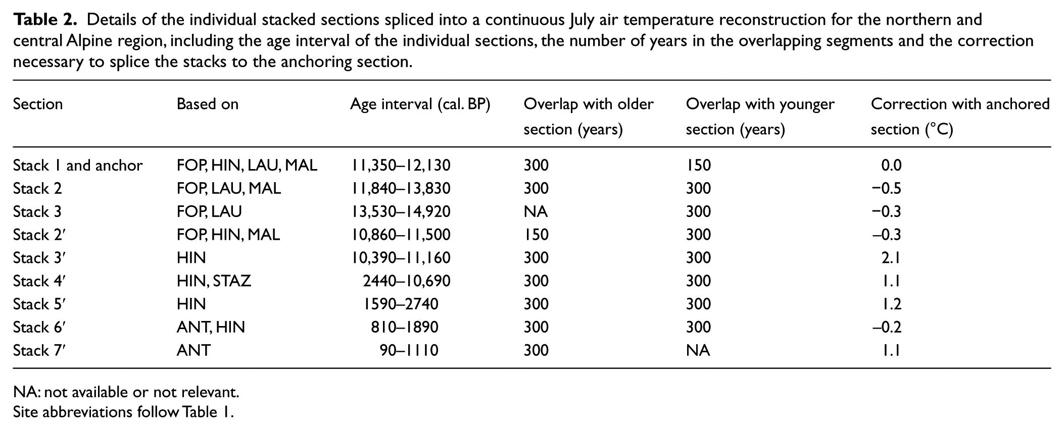
NA: not available or not relevant.

Site abbreviations follow Table 1.

The stacked record features a number of climatic events described in palaeoclimatic records in the Alpine region. These include the abrupt temperature increase at the beginning of the Lateglacial Interstadial at ~14,700 cal. BP (e.g. Von Grafenstein et al., 1999), the cooling at the start of the Younger Dryas episode and the rapid temperature increase at the transition to the Holocene (e.g. Lotter et al., 2000), cooler temperatures in the earliest Holocene compared with later periods, as supported by lower treelines reported for the earliest Holocene (e.g. Tinner et al., 1996), and the decrease in late Holocene temperatures starting after ~4000 cal. BP which coincides with the onset of Neoglaciation in the Alpine area (e.g. Leemann and Niessen, 1994). In contrast, shorter decadal- to centennial-scale climatic events, which have been reported for the region, are largely lacking. For example, the cooling episodes during the Lateglacial Interstadial such as the Gerzensee or Aegelsee Oscillation (e.g. Lotter et al., 1992), or the 8.2 kyr event (e.g. Von Grafenstein et al., 1999), are not visible in the reconstruction. This is partly because these events are not well expressed in the individual chironomid records (Figure 4a), but also because of the smoothing effect of the applied stacking procedure. Centennial- to millennial-scale temperature trends during the Holocene are more pronounced than in earlier chironomid-based reconstructions from the Swiss Alps (e.g. Heiri et al., 2004), with a ~1°C warming in the early Holocene and a ~2.5°C long-term cooling trend registered during the late Holocene (Figure 4d). Mid-Holocene July air temperatures (generally in the range of 16.5–17.5°C) are close to but slightly exceed expected values based on the position of the Alpine treeline in the Bernese Alps, Switzerland, in the mid-Holocene (7.9–11.1°C inferred for 2000 m.a.s.l; 13.9–17.1°C if corrected to 1000 m.a.s.l; Heiri et al., 2014b). July air temperatures of 14–15°C inferred for 1000 m.a.s.l in the youngest part of the reconstruction agree well with instrumental measurements of 17.6–18.7°C recorded for the 18th to 19th century at Basel Binningen, Northern Switzerland (30-year means, equivalent to 13.6–14.6°C at 1000 m.a.s.l; data from http://www.knmi.nl).

Errors for the stacked reconstruction have been calculated as the square root of the mean of the squared standard errors of prediction of the individual records that form a stack (Table 1) and range from 1.37°C to 1.70°C (Figure 5a). These error estimates represent the uncertainties associated with calculating quantitative temperature estimates based on chironomid assemblage data but do not include other potential error components such as, for example, chronological uncertainties or past changes in temperature lapse rates. For comparison, we also calculated the stacked reconstruction including the sections of the Hinterburgsee and Stazersee records that were affected by human impact, but excluding the section from Lac Anterne (Figure 5b). The two reconstructions are identical for the period older than ~2000 cal. BP. In the last ~1500 years, the latter reconstruction infers distinctly warmer temperatures than ~2000–3000 cal. BP, which conflicts with other palaeoclimate records that indicate that the past ~600 years included the coolest climatic conditions of the late Holocene (e.g. Ivy-Ochs et al., 2009). Considering the clear evidence for human impact on the chironomid records of Stazersee and Hinterburgsee, we consider the youngest 2000 years of this reconstruction unreliable.

Advantages, limitations and assumptions of the approach

The stacked and spliced chironomid reconstruction from the Alpine region (Figure 5a) provides a suitable example to illustrate both the potential and some of the limitations of the approach. In this reconstruction, the most serious limitation is obviously the number of records available for stacking within different sections of the time window of interest. The Lateglacial and early Holocene part is based on three to four different chironomid records, and variations recorded in individual sequences only are therefore reduced or offset by variability (or lack of variability) in the other sequences. However, for some section of the reconstruction, values are based on only two or in a few cases a single record (Figure 5). Clearly, such sections are less reliable and more susceptible to artefacts and variations in reconstructed values that are not representative of the regional climate. For example, both the inferred warming in the early Holocene and the gradual decrease in chironomid-inferred temperatures from ~4000 cal. BP onwards is based on variations in two records only (Hinterburgsee and Stazersee). The early Holocene increase is registered in both sequences simultaneously (Figure 4a). However, in the section of the Foppe record which was ignored when producing the stacked reconstruction, since this would have increased the number of splicings, no similar increase is apparent (data not shown). This may be because of a different regional climate in the region of Foppe than experienced at Stazersee and Hinterburgsee. Nevertheless, since this increase is an important feature of our reconstruction, it would be important to reproduce it in other records close to Stazersee or Hinterburgsee. A similar situation is apparent for the late Holocene cooling. The gradual cooling in the stacked reconstruction (Figure 5a) is the result of a gradual decrease of relatively low amplitude at Hinterburgsee and a more rapid, higher amplitude cooling inferred at Stazersee. Again, additional records from the same regions are needed to confirm the rate and the amplitude of this late Holocene cooling trend. The interpretation of such features in the stacked and spliced reconstruction presented in this study is complicated by the large distance between the individual sites. Differences between individual records, such as those from Hinterburgsee and Stazersee, could represent real differences in regional climate development between the Bernese Alps and the Eastern Swiss Alps. Alternatively, deviations between the two records could also be because of the effects of confounding variables on chironomid-based temperature reconstruction. The stacking and splicing procedure described here will be more powerful and easy to evaluate in instances when several (e.g. 3–5) reconstructions are available from the same region (e.g. the same valley or massif), since mean summer air temperature variability is not expected to vary significantly on such local scales. Variations in stacked and spliced reconstructions caused by variability in one of the records only will therefore point towards local processes rather than regional climatic effects.

The major advancement of the described stacking and splicing method compared with the more conventional smoothing methods (e.g. loess or spline smoothers) that can also be applied to reconstructions from multiple sites (e.g. Seppä et al., 2009) is the splicing procedure. This splicing has been designed to counter the effects of limited sequence lengths and discontinuous sequence availability on the stacking procedure, since, as discussed in detail above, this can cause biases if records which infer on average warmer or colder temperatures are only available for some sections of the reconstruction. However, the splicing procedure in itself may introduce artefacts into the reconstructions. On the one hand, this may happen at the splice itself when different stacks are amalgamated. However, biases may also occur if several records with low frequency variations are spliced so that maxima in the anchoring section coincide with minima in the section to be spliced to the anchor (or vice versa). If the next splice is again from a local maximum to a minimum in the next section to be spliced, then this can cause a gradual rise in inferred temperature in the stacked and spliced reconstruction. Such a ‘drifting’ in the stacked sequence (towards warmer values in the example outlined here) may exceed the overall rise in inferred temperatures in the individual records. The likelihood of such an effect influencing the reconstruction can be reduced by ensuring that individual stacks consist of more than 1–2 records and by reducing the number of splices between individual stacked sections as much as possible. Nevertheless, stacked and spliced reconstructions should be carefully evaluated, and it should be apparent which characteristics in the original records lead to prominent shifts in the stacked reconstruction. For example, in the stacked and spliced chironomid reconstruction from the Alpine region (Figure 5a), the early Holocene temperature increase at ~10,300–10,400 cal. BP and the late Holocene decrease after ~4000 cal. BP are clearly a consequence of variations in both the Hinterburgsee and Stazersee records with the higher amplitude variability in the Stazersee record leading to a more pronounced shift in temperatures than reported from some other Holocene temperature reconstructions from the Swiss Alps (e.g. Heiri et al., 2004). A further disadvantage of the presented approach is that the stacking procedure may mask unusual features and discrepancies in the chironomid records that may point towards biases and problematic sections. The results of the stacking procedure will nevertheless be influenced and potentially biased by such sections. Screening of the records, checking for consistency between individual records and elimination of problematic sections prior to stacking and splicing are therefore critical steps in this approach.

As with other smoothing and stacking methods, the approach we describe here assumes that reconstructed values included in the multi-site reconstruction are comparable. Quantitative temperature reconstructions are on the same temperature scale (°C), and this assumption may seem irrelevant. However, estimates based on different proxy types may differ systematically (e.g. Lotter et al., 2012), for example, if they are calibrated to the same temperature variable (e.g. July temperature) but represent different seasonal aspects of ‘temperature’ (e.g. mean summer temperatures, growing degree days, mean annual temperature). Furthermore, reconstructed temperatures based on different calibration datasets and transfer functions may also show systematic offsets (e.g. Engels et al., 2014; Lotter et al., 1999), because the training sets encompass different temperatures ranges. Since our stacking and splicing procedure corrects for offsets between different stacked sections, it can, to some extent, correct for such method-dependent offsets between datasets. As long as the different records have a similar sensitivity to past temperature change, variations in the stacked and spliced temperature records will correctly represent past temperature variations, even if the absolute values are affected. This situation may, for example, occur if temperature records based on different transfer functions and covering different sections of the time window of interest are included in the reconstruction. Even though we took care to taxonomically harmonize our records, and to recalibrate all chironomid reconstructions with the same transfer function, our approach would in principle also be applicable to more heterogeneous datasets consisting of temperature estimates based on different transfer functions or even different proxy types.

In our stacking and splicing procedure, absolute values are corrected to reflect the mean values of the records forming the anchoring section of the stacked and spliced reconstruction. This is an adjustment inherent to our approach, which typically does not influence other smoothing and stacking methods. It is important to take this correction into account when interpreting the results. In extreme cases, this may lead to situations where temperatures are adjusted to values typical for a region which is not represented in older or younger sections of the stacked record. For example, in the chironomid-based stacked and spliced reconstruction from the Alpine region (Figure 5a), the youngest section is based on the Lac Anterne record from the western French Alps. However, absolute temperatures are adjusted to represent average values of the anchoring section, which is based on records from the Central and Northern Swiss Alps and the French Jura (Table 2). However, the entire stacked and spliced record can also be anchored to other segments, or to other palaeotemperature data (e.g. instrumental records), if this is more appropriate to resolve the research question at hand.

A further silent assumption of our approach is that the lapse rates we used to correct July temperatures to 1000 m.a.s.l are representative for the entire time window encompassed in the reconstruction and did not change during the past ~15,000 years. The value of 6°C per 1000 m is widely used for altitudinal corrections in palaeo-studies and for model-to-palaeodata comparisons (e.g. Heiri et al., 2014b; Renssen et al., 2009; Samartin et al., 2012b). At present, lapse rates of air temperature are relatively constant in the Swiss Alps during the summer months (e.g. Livingstone et al., 1999). However, it can be expected that large-scale reorganizations of the climate system will lead to changes in adiabatic winds and precipitation patterns in mountain landscapes, processes which could influence long-term averages of temperature lapse rates. Therefore, summer temperature lapse rates may have been variable during the Holocene and Lateglacial in parts of the Alpine regions. A further problem may develop for stacked and spliced reconstructions if past temperature events changed in amplitude with elevation. If the reconstructions are based on low-elevation sites in some time intervals and high-elevation sites in others, this may lead to variations in the amplitude of reconstructed temperature change in different sections of the stacked reconstructions which do not reflect true shifts in the temperature variability with time. However, the issues discussed here, that is, the assumption of constant lapse rates and problems associated with changing amplitudes of climatic change with elevation, do not only influence our stacking and splicing procedure but affect any comparison, smoothing or stacking of temperature records obtained at different elevations in mountain regions. At present, hardly any information is available on past changes in temperature lapse rates in the Alpine region, and this problem deserves further attention.

Future developments

We have shown that discontinuous temperature records from lake sediment sequences can be combined to continuous reconstructions based on the stacking and splicing procedure presented in this study. Furthermore, we have demonstrated that these stacks approximate smoothed palaeoclimate records if based on a sufficient number of individual sequences, and that reconstructions based on a relatively low number of individual records (e.g. 4–5) can already capture most of the multi-centennial to millennial-scale variability that would be apparent in continuously sampled, high-resolution reconstructions over the same time window. However, our simulation experiments have also revealed that the presented approach, even if dating uncertainty in the individual records is ignored, is less successful at reconstructing decadal- to centennial-scale variability. Furthermore, as discussed above, stacked reconstructions based on a few records only may still be strongly influenced by climatic variability restricted to individual records, and in these sections, the stacked record may not be representative for past variations in regional climate.

The stacking and splicing procedure we describe is well suited for developing long and continuous regional reconstructions of past temperature change during the late Quaternary. For chironomid records in the Alpine region, the example we examine in this publication, the obvious limitation for the approach is the limited number of chironomid records available. Our dataset could have been expanded to some extent by including some additional records from the Swiss Plateau calibrated using a different transfer function (e.g. Egelsee, Larocque-Tobler, 2010), or from sites which were not included since evidence suggests that their chironomid records may have been influenced by local, site-specific effects (e.g. Sägistalsee, Heiri and Lotter, 2003; Gerzensee, Lotter et al., 2012). However, this would not change that the records available for stacking are dispersed over a relatively large region and that, because of the widespread impact of human activity on lakes and landscapes, only few reliable reconstructions are available for the late Holocene. We therefore believe that the following steps would be essential to further develop and improve the stacked and spliced chironomid-based temperature reconstruction in the Alpine region: