Study of the distribution of Elphidium aff. poeyanum (D’ORBIGNY) and Buccella peruviana (D’ORBIGNY) from the Colorado basin (South America): Holocene paleoenvironmental inferences

Abstract

Benthic foraminiferal assemblages recovered from T1 core samples of the Colorado basin, in the continental margin of southeastern Argentina, were analyzed to understand their distribution patterns and ecological preferences. The foraminiferal assemblages showed two well-represented species: Elphidium aff. poeyanum (d’Orbigny) and Buccella peruviana (d’Orbigny), among others of very low proportion. Statistical analyses allowed identifying positive correlations between the abundance of E. aff. poeyanum and silt content and between B. peruviana and the sand content, reflecting better conditions for the development of both species. From a paleoenvironmental point of view, the assemblages recorded are characteristic of an inner shelf, showing a passage from typical shallow waters to normal marine conditions; such a passage represents a rise in the sea level during the post-last glacial maximum transgression. The results obtained contribute to the knowledge of South American foraminifers and paleoenvironments during the Holocene.

Keywords

Holocene paleoenvironmental changes sea level changes

Introduction

Foraminifers are organisms that, because of their widespread geographic distribution and specific environmental requirements, are used as paleoecological bioindicators of marine environments. Several ecological studies of benthic foraminifera have been carried out to explain the patterns of distribution and dynamics of communities (Murray, 2001). They are also used to provide data to establish proxy relationships with selected factors. At any one time, the factor or factors close to the threshold of tolerance for any given species are those that will limit its local distribution. Benthic foraminifera have the potential to operate as proxies of environmental factors; this involves co-variation between either the abundance of an organism or the composition of an assemblage of organisms and a given environmental parameter (Murray, 2001). Therefore, these microfossils are potentially excellent paleoenvironmental proxies, especially to detect variations which occurred in the marine environment because of sea level changes during the Holocene (Berkeley et al., 2007; Schnack et al., 2005). Different environments characterized by a certain parameter could be revealed through foraminifers. Some pioneering researchers have used benthic foraminifera as indicators of oceanic circulation (Armstrong and Brasier, 2008; Boltovskoy, 1976, 1981; Boltovskoy et al., 1980; Kahn and Watanabe, 1980), whereas others have used them to determine paleoxygenation levels (Bernasconi and Cusminsky, 2009; Bernasconi et al., 2009; Kaiho, 1994, 1999). Earlier observations indicated the influence of the sediment on the distribution of foraminifera (Boltovskoy, 1963). Then, the probable incidence of other parameters such as temperature, salinity, depth, organic matter was analyzed by several authors (Alperin et al., 2008, 2011; Bernasconi and Cusminsky, 2005; Bernhard, 1986; Boltovskoy, 1965; Boltovskoy et al., 1991; Corliss and Chen, 1988; Gary et al., 1989; Loubere, 1997; Yanko et al., 1998). Hayward et al. (1996) considered that the mud content was one of the factors that most affects the distribution of recent foraminifers. Murray (1991) and Hayward et al. (2002) analyzed the distribution patterns of benthic foraminifera and suggested that the most important parameter was the substrate grain size which is related to the depth and the type of sediments.

Numerous researches on foraminifers were carried out in the Atlantic coast of South America. In Argentina, Boltovskoy studied the foraminifera fauna both from restricted areas such as San Jorge Gulf and San Blas Bay (Boltovskoy, 1954a, 1954b), and from estuary environments like Río de La Plata estuary (Boltovskoy, 1957), and also described the most important species and assemblages of foraminifers in coastal areas of Argentina (Boltovskoy et al., 1980). Other studies have recorded foraminifers near the area studied in the present work (Colorado basin) and documented paleoecological and paleoenvironmental inferences (Alperin et al., 2008, 2011; Becker and Bertels, 1980; Bernasconi, 2006; Bernasconi and Cusminsky, 2005; Bernasconi et al., 2009; Calvo Marcilese et al., 2011; Calvo Marcilese and Pratolongo, 2009; Caramés and Malumián, 2000; Cusminsky et al., 2006, 2009; Ferrero, 2006, 2009; Laprida, 1998; Laprida and Bertels-Psotka, 2003; Laprida et al., 2007, 2011; Malumián and Náñez, 1996).

Sedimentological aspects of the core T1, which is located in the submarine Colorado Basin were analyzed by Gelós and Chaar (1988). They mentioned that the lower levels constituted by silty clay sediments corresponded to a deposition in shallow waters of the littoral of marshes and ponds. Instead, the upper levels were characterized by sandy sediments suggesting a coastal littoral environment with tide regimens and coastal currents. In micropaleontological T1 core, two zones were recognized, one in the lower levels and other in upper levels. The first was represented by a dominance of Elphidium discoidale that is common in shallow waters and low values of diversity. However, the second zone was characterized mainly by Buccella peruviana f. campsi together with more high values of diversity which was interpreted as a marine condition (Bernasconi and Cusminsky, 2007).

E. discoidale in Argentinean coastal waters was recently reassigned as Elphidium aff. poeyanum in marginal marine and restricted environments (Calvo Marcilese, 2011; Calvo Marcilese et al., 2011, 2013). While B. peruviana f. campsi was considerate a stage in the develop of B. peruviana (Calvo Marcilese and Langer, 2012).

The purpose of this work was to analyze the relationship between the distributions of E. aff. poeyanum and B. peruviana with the type of sediments along the core. Paleoenvironmental implications such as sea level fluctuations which occurred during the early Holocene are described.

Environmental setting

General characteristics

The core T1 is located in the Colorado basin (40° 30′S and 60° 59′ 05″W). This basin is placed in the SE coast of Buenos Aires province (Argentina) and spreads toward the east on the submarine continental shelf. The area has a surface of 35,000-km² inner coast and 95,000-km² outer coast and maximum width of sediments of 7000 m (Urien and Zambrano, 1996). The Colorado basin constitutes a group of basins of Atlantic margin, which originated during the Upper Jurassic–early Cretaceous, associated with the opening of the South Atlantic ocean (Fryklund et al., 1996).

The stratigraphical sequence belongs to a Permian basement, above of this, Fortín Formation (late Jurassic–early Cretaceous) was deposited, after in angular discordance Colorado Formation (early–late Cretaceous) was lying. The sequences continue with Pedro Luro Formation (deep marine environment) overlying in erosive discordance (Maastrichtian–Paleocene), and over it are two formations: the Ombucta (Eocene) and Elvira (deep marine environment except near of Bahía Blanca; Oligocene) Formations. Then, the Barranca Final Formation corresponding to the Oligocene–Pliocene is superposing in discordance according to a shallow to batial environment. The last is the Belén Formation, corresponding to the Pliocene–Quaternary characterized by not consolidated sediments and shale of marine environment (Caramés and Malumián, 2000; Fryklund et al., 1996).

Topography

The topography has a slow NW to SE gradient. The relief is very scarce or null up to a depth of 70 m; from there up to 140 m the topography presents few undulations. At greater depths up to the slope the irregularities are strongly marked (Cortelezzi and Mouzo, 1979; Gelós et al., 1988; Mouzo, 1982; Mouzo et al., 1974; Figure 1).

Figure 1.

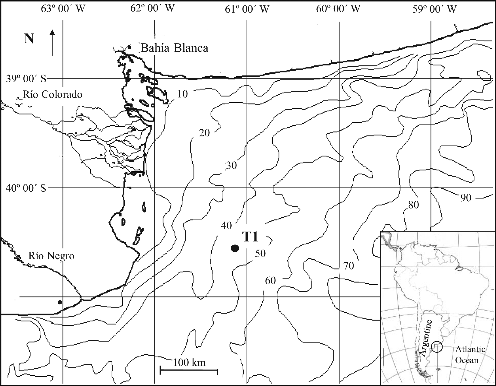
Location map (bathymetry modified to Gelós et al., 1988).

Hydrography

The hydrology of this area is complex. This area is wide from the coast up to the isobaths 80–100 m and is related to the Argentinean Coast water system, called Patagonian current, and influenced by winds and currents in North direction (Cortelezzi and Mouzo, 1979; Mouzo et al., 1974). This water mass has sub-Antarctic origin, its surface temperature varies between 9°C and 20°C, and its salinity presents a seasonal and latitudinal variation, between 33 and 33.5 psu (Boltovskoy, 1981). Martos and Piccolo (1988) differentiated two water mass domains on the shelf: a coastal or inner domain and an outer domain. The first one includes the littoral zone down to the isobaths of 40–50 m with vertically homogeneous waters. In this area, Guerrero and Piola (1997) and Lucas et al. (2005) recognized a first coastal water in El Rincón estuary with low salinity (S < 33.4 psu) formed by the discharge from the Negro and Colorado rivers and a second coastal water with high salinity (33.8–34.0 psu) located near the coast area east of El Rincón estuary. The coastal area is bounded to the east by the coastal front (Guerrero, 1998; Guerrero and Piola, 1997; Lucas et al., 2005), which separates it from the continental waters of the shelf. Coastal circulation is from SSW to NNE. The outer domain lies between 40–50 m and 100-m depth at the top of the continental slope. This domain is characterized by the Middle Shelf Water (S between 33.4 and 33.6–33.7 psu), comprising the northwards-flowing Patagonian current (Guerrero and Piola, 1997). These waters are homogeneous in winter and stratified in summer. Surface waters have temperatures and salinity typical of the de la Plata River (T° > 15°C; S < 33 psu) in the spring–summer months, flowing southwestward. In the autumn–winter months, the surface waters are cooler (T° mean 12°C) and the water column is vertically mixed by convection and influenced by the cold waters (<15°C) and has relatively low salinity (34.2 psu) from Malvinas current. The salinity values are typical of a continental shelf (Alperin et al., 2008, 2011; Martos and Piccolo, 1988). The water masses control zoogeographical distribution (Boltovskoy et al., 1980). A zoogeographic division of South America on the basis of foraminifera was presented by Boltovskoy (1976), who determinates four provinces: West Indian, Argentine, Chilean–Peruvian, and Panamanian. The Colorado basin is in Argentine province that is divided into two subprovinces, Nord Patagonic and South Patagonic. These subprovinces are mainly distinguished by two species of genus Elphidium (E. discoidale and E. macellum) that is common to the shallow shelf areas (Boltovskoy, 1981). The T1 core is located specifically in the Nord Patagonic subprovince placed between 32° and 42–43° S, and the southern limit coincides with Valdez peninsula which is characterized fundamentally by E. aff. poeyanum. South from this area, in the South Patagonic subprovince, Elphidium macellum is characteristic.

Sediments

The sediment is texturally mature and compositionally homogeneous. It is well-selected and constituted by fine to very fine sand. The present distributive dynamics would be related to the shelf currents with N and NE directions (Gelós et al., 1988). The sediments from deltaic and estuary deposits are re-transported by the littoral drift of semi-permanent currents along the coastline (Gelós et al., 1988). In this zone, the Colorado and Negro Rivers have a great influence because of their currents and suspended load capacity in the Holocene. The migration of the coastline toward the west and the invasion of the coastal flats occur during the transgressive stage. The current littoral morphology is dominated by destructive characters because of the influence of waves and tides, particularly in the delta of the Colorado River to the south of Bahía Blanca (Gelós et al., 1988).

Materials and methods

Samples

The T1 core, located at 40° 30′ S and 60° 59′ 05″ W, is 4.33-m long. It was extracted by the Puerto Deseado ship during the campaign in 1984 by Argentine Institute of Oceanography, at a depth of 45 m below sea level (Bernasconi and Cusminsky, 2007; Figure 1). From the base of the core up to 425 cm, there are fine and washed materials with a predominance of rest of shells, sand, and clayey sediment. Between 425 and 230 cm, a sequence of dark silty clay to gray-greenish clay with rest of shells is observed. Between 230 and 185 cm, the size of sediments increases from sandy silt to silty clay. From 185 cm up to the top of the core, sandy sediments are recognized. When wet, their color changed from light grayish to dark grayish, and they had rest of shells with intercalation of silty clay materials (Gelós and Chaar, 1988).

Radiocarbon dating (AMS) set the age of the sequence at 10,027 ± 56 yr BP for the lower section (Level 385 cm – AA61785; 9427 ± 56 cal. yr BP) and at 9514 ± 86 yr BP for the upper section (Level 85 cm – AA61786; 8914 ± 86 cal. yr BP; Bernasconi and Cusminsky, 2007).

Benthic foraminiferal and sedimentological analyses

The core was sampled approximately each 10 cm from bottom to the top. Thirty-one samples were washed through a 63 µm (Tyler Screen System N° 230). Systematic analysis of genera was based on Loeblich and Tappan (1992), for species was based on adequate bibliography. Scanning electron microscope (Philips SEM 515) pictures were taken at Centro Atómico Bariloche, Argentina. Quantitative values such as total abundance, relative abundance, and diversity index were determined (Bernasconi and Cusminsky, 2007). The specimens collected are stored at the repository of the Museum of Natural Sciences and National University of La Plata (Buenos Aires, Argentina) under the initials MLP-Mi and numbers 1784–1795. Bulk sediment was applied to analyze the grain size. Sieve n° 30 and 10 were used to separate the different fractions (gravel, sand, and silt).

Statistical analysis

In order to analyze joint variations of the two predominant species, and the type of sediment, the ratios between percentages of E. aff. poeyanum and B. peruviana and percentages of silt and sand content were determined. Also, to determinate the relationship between E. aff. poeyanum and B. peruviana with the sediment, the correlation between both ratios was calculated and expressed as the following correlation (percentage E.p./percentage B.p., percentage silt/percentage sand).

Based on these data, the relationship between both species and the type of sediments was analyzed. Non-parametric analyses were performed using Spearman’s rank correlation coefficient. These analyses order and convert the values of Xi and Yi to xi and yi ranks, di = rank of xi − rank of yi, and n = number of data. The Spearman coefficient is represented by the equation: Rs = 1 − 6(di)²/(n(n² − 1)).

The high quantity of E. aff. poeyanum species allowed us to make an analysis of size frequency related to the sediment characteristics. Fauna data consisted of 1500 specimens of E. aff. poeyanum that were measured to document the frequency of sizes. On the other hand, in the case of B. peruviana, its abundance was very low to analyze frequency of sizes. The correlation between range sizes (Max value − Min value) with the sediment characteristics expressed as the ratio of percentage silt and percentage sand of the population at every sampled level was carried out.

Results

The sediments were constituted by mud, sand, and gravel in different proportions. The percentage of mud (clay and silt) varied between 99% at 275 cm and 4.7% at 30 cm. The proportion of sand varied between 94% at 74 cm and 1% at 275 cm. The gravel content was scarcely distributed, varying between 0.1% at 370 cm and 40% at 30 cm. At 320, 290, 275, 245, and 230 cm, gravel was absent.

The most represented species were Elphidium aff. poeyanum and Buccella peruviana. E. aff. poeyanum was found in 26 levels. E. aff. poeyanum dominated in the lower levels, representing more than 55% of total abundance (Figure 2). Toward the top, the relative abundance of B. peruviana, and the diversity increased to the detriment of E. aff. poeyanum.

Figure 2.

Elphidium aff. poeyanum (d’Orbigny); 1 – MLP-Mi 1784. 2 – MLP-Mi 1785. 3 – MLP-Mi 1786. 4 – MLP-Mi 1787. 5 – MLP-Mi 1788. 6 – MLP-Mi 1789. 7 – MLP-Mi 1790. 8 – MLP-Mi 1791. 9 – MLP-Mi 1792. 10 – MLP-Mi 1793. 11 – MLP-Mi 1794. 12 – MLP-Mi1795. Scale 100 µm (1, 2, 4, 5, 6, 7, 8, 10, 12), 50 µm (3, 9, 11).

Thus, the ratio between E. aff. poeyanum and B. peruviana and the ratio between silt and sand presented values higher in the lower levels than in the upper levels, reflecting high percentages of E. aff. poeyanum and silt, respectively. Both ratios (percentage E.p./percentage B.p.) and (percentage silt/percentage sand) registered a positive correlation (Rs = 0.73; p = 0.0002). This correlation showed tendencies that reflect a high abundance of E. aff. poeyanum in lower levels (400–275 cm) where the percentage of silt is higher than the rest of the core and a very low percentage of E. aff. poeyanum where the sand content is high (Figure 3).

Figure 3.

Plot showing the correlation between the ratios of percentage of both species and ratio of percentage silt/percentage sand expressed as correlation (percentage E.p./percentage B.p., percentage silt/percentage sand).

The distributions of E. aff. poeyanum and B. peruviana along the core were heterogeneous; for this reason, the relationship between the percentage of both species and the type of sediment was analyzed. For this purpose, the nonparametric method of Spearman coefficient was applied. Spearman Rank correlations comparing sediment sample parameters at all levels indicated that E. aff. poeyanum was highly significantly correlated with silt content (Rs = 0.72, p = 0.00005). The correlation between E. aff. poeyanum and sand content was Rs = −0.69 (p = 0.00001), whereas that with gravel content was Rs = −0.52 (p = 0.0001). Spearman coefficient between B. peruviana and mud was Rs = −0.62 (p = 0.0002), whereas that with sand content was Rs = 0.57 (p = 0.0007) and that with gravel was Rs = 0.3 (p = 0.04). This showed that E. aff. poeyanum was positively correlated with silt content. E. aff. poeyanum showed a negative correlation with sand and gravel content. The opposite occurred with B. peruviana: its presence was positively associated with sand content and negatively associated with mud. The proportion of B. peruviana was not correlated with gravel.

With respect to the range of sizes of E. aff. poeyanum, a large amplitude was observed. The sizes varied from 100 to 800 µm. Larger ranges were recorded at 385 cm up to 320 cm, being the median value 400 µm (Figure 4). This distribution agrees with the highest percentage of mud, lowest of sand and gravel content. Total abundance values at these levels were highest as well. However, from 433 to 400 cm and 310 cm up to top of the core, the amplitude of the range was smaller and the median value was 280 µm. At these levels, the range decreased, in agreement with an increase in sand and gravel content in relation with silt content. On the other hand, the correlation between range sizes (Max value − Min value) with the ratio (percentage silt/percentage sand) was Rs = 0.65 (p = 0.001), showing a positive significant correlation (Figure 5).

Figure 4.

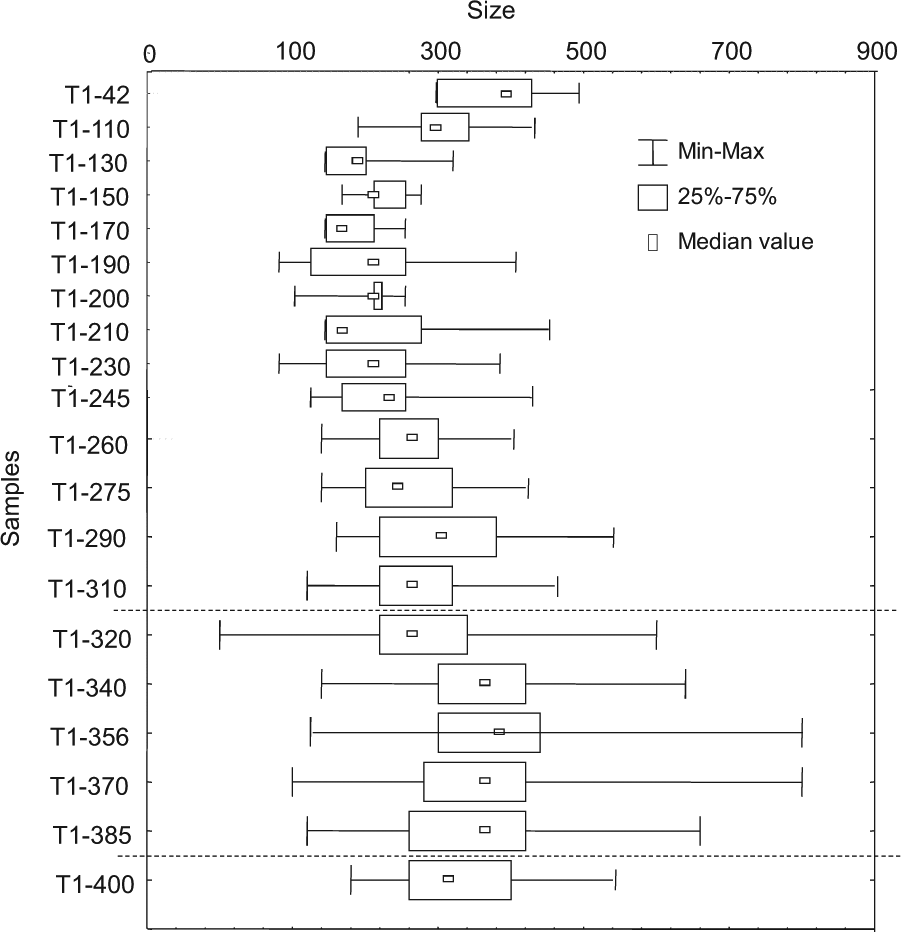
Box plots showing maximum, minimum, inter-quartile ranges, and median size (µ) populations of E. aff. poeyanum in each sample. The largest range sizes of the population shown between dotted lines.

Figure 5.

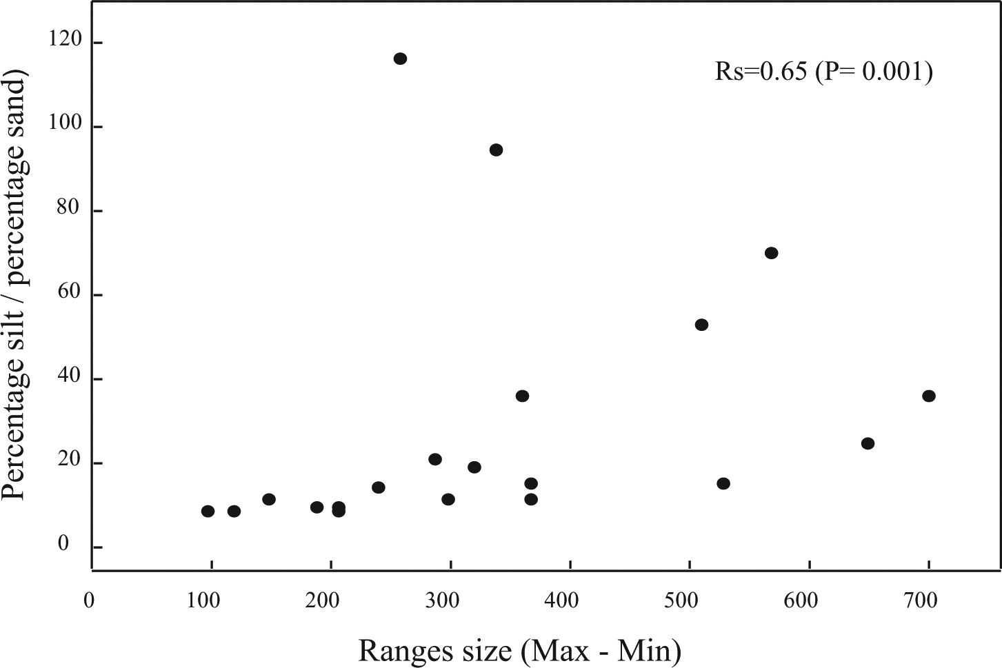
Graphics of the correlation between range sizes (Max value – Min value) and ratio of percentage silt/percentage sand expressed as correlation (percentage E.p./percentage B.p., percentage silt/percentage sand).

Discussion

In this study, two well-defined assemblages were shown, one of them dominated by E. aff. poeyanum and the other represented mainly by individuals of B. peruviana which were significantly related with different grain sizes of sediments along the core. The genus Elphidium is epifaunal on sand or vegetation, is typical of the inner shelf from 0 to 50 m of depth rarely batial and lives in temperate-warm waters. In addition, it exhibits wide salinity tolerance as eurihaline genus. This genus is found in brackish-hypersaline bays, marshes, lagoons, estuaries, and inner shelf (Murray, 1991).

In particular, E. aff. poeyanum is very common in shallow shelf areas of the northern part of the littoral zone of the Argentine Province up to 41° S, typical of warm-water species (Boltovskoy, 1965, 1970; Boltovskoy et al., 1980). This species dominates the North Patagonian subprovince (Boltovskoy, 1976, 1979; Boltovskoy and Totah, 1985; Boltovskoy et al., 1980). It has been found in littoral environments (Alperin et al., 2008; Bernasconi, 2006; Bernasconi and Cusminsky, 2005, 2007), and in hyposaline lagoons and estuaries and brackish environments, both as modern and fossil sediments (Boltovskoy, 1976; Calvo Marcilese and Pratolongo, 2009; Calvo Marcilese et al., 2011; Cusminsky et al., 2006; Laprida et al., 2007, 2011; Márquez and Ferrero, 2011).

The genus Buccella is widely distributed in coastal waters of Argentina from 32–33°W to 57–58°S (Boltovskoy et al., 1980). Buccella is registered in inner shelf between 0 to 100 m and cold temperate waters (Murray, 1991). Buccella peruviana is the most common species that inhabits the Argentinean zoogeographic province (Boltovskoy, 1970, 1976; Boltovskoy et al., 1980; Theyer, 1966). This is found in marginal, marine, and restricted environments of Argentina, Brazil, and Uruguay (Bernasconi, 2006; Boltovskoy, 1976; Boltovskoy and Lena, 1974; Boltovskoy et al., 1980; Calvo Marcilese et al., 2013; Cusminsky et al., 2006, 2009; Ferrero, 2006; Márquez and Ferrero, 2011, among others). Buccella peruviana included the forms campsi and frigida which are different stages of the development of the same species.

The new information led to the determination of two 2-zone cores, T1-A which was divided into two subzones T1A-I, T1A-II, and T1-B (Figure 6). In the first, T1A-I was represented by a very low abundance of B. peruviana associated with sandy silty clay sediment. That was probably due to an increase in the energy by local issues. In T1A-II, E. aff. poeyanum dominated and higher range of size distributions were associated with silty clay sediments that reflect characteristics of shallow waters and low-energy conditions. In contrast, toward the top of the core (T1-B), a gradual increase in the abundance of B. peruviana correlated with a gradual increase of sand and gravel sediment, and diversity values suggested an increase in the energy of environment. The passage from a shallow environment of low energy to normal marine conditions of higher energy points to a transition and change environment related with an increase in the sea level in the early Holocene.

Figure 6.

Paleoenvironmental interpretation showing zones and subzones related with the lithology, ages, and curves with the ratio of percentage E. aff. poeyanum and percentage B. peruviana (% E.p./% B.p.) and the ratio of percentage silt and percentage sand (% silt/% sand).

All the above mentioned was revealed from benthic foraminifera which can operate as proxies of environmental factors. This involves co-variation between either the abundance of an organism or the composition of an assemblage of organisms and a given environmental parameter (Murray, 2001, 2006). The type of sediment is considered a relevant parameter that influences the development and distribution of benthic foraminifera (Bernhard, 1986; Boltovskoy, 1963, 1965; Hayward et al., 2002; Schmiedl et al., 1997; Severin, 1983; Yanko et al., 1998). Corliss and Chen (1988) evaluated epifaunal and infaunal patterns related to water mass distribution, grain size composition, and organic carbon content and related Elphidium spp. with silty sediments. In Argentina, B. peruviana in zones characterized by sand sediments was cited (Alperin et al., 2008, 2011). In another study, the distribution and size of Nonionella auris (d’Orbigny) were positively correlated with muddy sediment, suggesting more favorable conditions for its growth (Bernasconi and Cusminsky, 2005).

In reference to the association found in this research, E. aff. poeyanum together with B. peruviana is mentioned as characteristic of shallow water species from intertidal estuarine environments with oligohaline to mesohaline conditions (Brock, 1999; Debenay and Guillou, 2002; Hayward and Hollis, 1994; Ishman et al., 1996; Poag, 1978; Sen Gupta, 2002). This association was cited in some different environments of the Argentinean continental shelf. For instance, a study carried out by Cusminsky et al. (2006) recognized in Bahía Blanca estuary a restricted shallow environment with variation of salinity contents and related higher abundance of E. aff. poeyanum with high silt content. In a research conducted by Calvo Marcilese et al. (2011, 2013), B. peruviana and E. aff. poeyanum showed different conditions during the Holocene.

Boltovskoy and Totah (1985) cited B. peruviana and E. aff. poeyanum in coastal waters, and only B. peruviana in outer shelf recognized two water masses related with the variations of physical parameters. The prevalence of B. peruviana over E. aff. poeyanum was interpreted by Bernasconi and Cusminsky (2005), Cusminsky et al. (2006), and Gómez et al. (2005) as an increase in the marine conditions. Also, Laprida et al. (2007) and Cusminsky et al. (2009) related this foraminiferal assemblage with silty clay sediments and a low-energy fluvio-marine estuarine to near shore brackish environment. Ferrero (2009) reported assemblages constituted by E. discoidale (E. aff. poeyanum) and B. peruviana, between others, which suggested marginal marine environments in Mar Chiquita coastal lagoon (Buenos Aires province). Márquez and Ferrero (2011) cited marine influence in the early Holocene from Mar Chiquita lagoon related this change with a great silty sediments.

Paleoenvironmental changes and sea level fluctuations during the early Holocene

The Holocene sea level in southeastern South America is based on fluctuations in the sea level position. In Argentina, until the sea level reached the current configuration, it was not uniform and had strong local components (Fucks et al., 2005; Laprida et al., 2007; Schnack et al., 2005). Depositional sequences in the Río de La Plata River and adjacent marine and coastal regions were deposited in the context of a significant climate change from the end of the glacial epoch (Calvo Marcilese et al., 2011). A progressive sea level rise between 9750 and 8200 yr BP was recognized by Guilderson et al. (2000) from several cores located along the Argentine Continental shelf. Several authors have suggested that the sea level rise about 8000 yr BP and that at the age of 7000 yr BP might have been at the current level (Cavallotto et al., 2004; Violante and Parker, 2000, 2004; Violante et al., 2001). In coastal areas near the north of Argentina, the sea level presented a maximum ca. 6000 yr BP, when the shoreline was 5–12 m over the current level (Schnack et al., 2005). Márquez and Ferrero (2011) recognized the evolution of the environment related to sea level changes during the Holocene of Mar Chiquita Lagoon.

Finally, our results corroborated and supported a paleoenvironmental change based on a rise of the sea level ca. 9634 yr BP.

Conclusion

In this study, a preferential distribution of foraminiferal fauna is significantly correlated with the type of sediment. At lower levels, E. aff. poeyanum abundance and its wider range of size distribution were related to the silty substrate more favorable for its growth and development. Toward to upper levels of the core, a gradual passage from a shallow and low energy environment to normal marine conditions.

The paleoecological analysis from the Colorado basin suggests a Holocene evolution, in agreement with the regional trends, where deposits were accumulated during the early Holocene. The results obtained suggest that combined field data and model predictions are adequate to provide accurate reconstructions of the former sea level.

Footnotes

Acknowledgements

This work was performed at the Department of Ecology of the National University of Comahue and Instituto de Investigaciones en Biodiversidad y Medioambiente INIBIOMA, National Research Council (CONICET), Argentina, and constitutes a contribution to projects: Universidad Nacional del Comahue B166; CONICET PIPs 1122008010081, 11420199100234, 11220120100021, and to the National Agency for the Promotion of Science and Technology PICT BID 2010-0082. We are grateful to both reviewers for their suggestions and comments which enriched this paper.

Funding

This research received no specific grant from any funding agency in the public, commercial, or not-for-profit sectors.

References

Alperin

Bernasconi

Cusminsky

(2008) Asociaciones de foraminíferos bentónicos actuales de la plataforma continental argentina (39º-43ºS y 58º-65ºO) analizados con métodos estadísticos para datos composicionales. Ameghiniana 45: 443–461.

Alperin

Cusminsky

Bernasconi

(2011) Benthic foraminiferal morphogroup assemblages in recent sediments of the Argentine Continental Shelf (39º-43º S and 58º-65º W). Journal of Foraminiferal Research 41: 155–166.

Armstrong

Brasier

(2008) Microfossils. 2nd Edition. Malden, MA: Blackwell Publishing, 296 pp.

Becker

Bertels

(1980) Micropaleontologia de la secuencia terciaria de la perforacion Puelche (margen continental argentino). In: Actas 2° Congreso Argentino de Paleontologico y Bioestrafigrafia y I Congreso Latinoamericano de Paleontologia, Buenos Aires, 20 September 1978, pp. 315–333.

Berkeley

Perry

Smithers

. (2007) A review of ecological and taphonomic controls of foraminiferal assemblage development in intertidal environment. Earth Science Reviews 83: 205–230.

Bernasconi

(2006) Los foraminíferos del Holoceno de testigos de la plataforma continental argentina (40º 30′-42º 48′LS y 59º 25′-64º 40′LO). PhD Thesis, Universidad Nacional del Comahue, Argentina, 210 pp.

Bernasconi

Cusminsky

(2005) Distribución de Nonionella auris (d’Orbigny) Orden Foraminiferida en el Golfo San Matías, Provincias de Río Negro, Argentina. Ameghiniana 42: 167–174.

Bernasconi

Cusminsky

(2007) Estudio de los foraminíferos bentónicos de un testigo holoceno proveniente de la cuenca del Colorado. Ameghiniana 44: 271–278.

Bernasconi

Cusminsky

(2009) Estudio paleoecológico de Foraminíferos de testigos del Holoceno de Golfo Nuevo (Patagonia, Argentina). Geobios 42: 435–450.

10.

Bernasconi

Cusminsky

Gómez

(2009) Foraminíferos bentónicos del holoceno del golfo Nuevo, Argentina: Inferencias paleoclimáticas. Revista Española de Micropaleontología 41: 21–34.

11.

Bernhard

(1986) Characteristic assemblages and morphologies of benthic foraminifera from anoxic, organic-rich deposits: Jurassic through Holocene. Journal Foraminiferal Research 16: 207–215.

12.

Boltovskoy

(1954a) Foraminíferos del Golfo de San Jorge. Revista del Instituto Nacional de Investigación de las Ciencias Naturales y Museo Argentino de Ciencias Naturales Bernardino Rivadavia, Ciencias Geológicas 3: 79–228.

13.

Boltovskoy

(1954b) Foraminíferos de la Bahía San Blás. Revista del Instituto Nacional de Investigación de las Ciencias Naturales y Museo Argentino de Ciencias Naturales Bernardino Rivadavia, Ciencias Geológicas 4: 247–300.

14.

Boltovskoy

(1957) Los Foraminíferos del Estuario del Río de La Plata y su zona de influencia. Revista del Instituto Nacional de Investigación de las Ciencias Naturales y Museo Argentino de Ciencias Naturales Bernardino Rivadavia, Ciencias Geológicas 6: 1–78.

15.

Boltovskoy

(1963) Foraminiferos y sus relaciones con el medio. Revista del Museo Argentino de ciencias Naturales Bernardino Rivadavia Hidrobiología 1: 21–107.

16.

Boltovskoy

(1965) Los Foraminíferos recientes. Buenos Aires: Eudeba, Editorial Universitaria de Buenos Aires, 510 pp.

17.

Boltovskoy

(1970) Distribution of the marine littoral foraminifera in Argentina, Uruguay and Southern Brazil. Marine Biology 6: 335–344.

18.

Boltovskoy

(1976) Distribution of recent foraminifera of the South American region. Foraminfera 2: 171–236.

19.

Boltovskoy

(1979) Paleoceanografía del Atlántico Sudoccidental desde el Mioceno, según estudios foraminiferológicos. Ameghiniana 16: 357–389.

20.

Boltovskoy

(1981) Masas de agua en el Atlantico Sudoccidental. In: Boltovskoy

(ed.) Atlas de Zooplancton del Atlántico Sudoccidental. Buenos Aires: Inst. Nac. Inv. del Desarrollo pesquero Minero Comercial Internacional Marítimo Argentino, pp. 227–236.

21.

Boltovskoy

Lena

(1974) Foraminíferos del Río de La Plata. Revista del Servicio de Hidrografía Naval H 661: 3–22.

22.

Boltovskoy

Totah

(1985) Diversity, similarity and dominance in benthic foraminiferal fauna along one transect of the argentine shelf. Revue de Micropaleontologie 28: 23–31.

23.

Boltovskoy

Giussani

Watanabe

. (1980) Atlas of Benthic Shelf Foraminifera of the Southwest Atlantic. The Hague: W. Junk Publishers, 147 pp.

24.

Boltovskoy

Scott

Medioli

(1991) Morphological variations of benthic foraminiferal tests in response to changes in ecological parameters: A review. Journal of Paleontology 65: 175–185.

25.

Brock

(1999) Application of Foraminiferida in earth sciences. Geos 39: 1–6.

26.

Calvo Marcilese

(2011) Sistemática y Paleoecología de los foraminifera (Protista) del Holoceno el área del estuario de Bahía Blanca, Argentina. PhD Thesis, Facultad de Ciencias Naturales y Museo, Universidad Nacional de La Plata, 253 pp.

27.

Calvo Marcilese

Langer

(2012) Ontogenetic morphogenesis and biogeographic patterns: Resolving taxonomic incongruences within ‘species’ of Buccella from South American coastal waters. Revista Brasileira de Paleontologia 15: 23–32.

28.

Calvo Marcilese

Pratolongo

(2009) Foraminíferos de marismas y llanuras de marea del estuario de Bahía Blanca, Argentina: Distribución e implicancias ambientales. Revista Española de Micropaleontología 41: 315–332.

29.

Calvo Marcilese

Cusminsky

Gómez

(2011) Asociaciones de foraminíferos bentónicos en secciones holocenas del estuario de Bahía Blanca (Buenos Aires, Argentina). Ameghiniana 48: 210–225.

30.

Calvo Marcilese

Pérez Panera

Cusminsky

. (2013) Micropaleontological record of Holocene estuarine stages in the Bahía Blanca estuary, Argentina. Journal of South American Earth Sciences 45: 147–159.

31.

Caramés

Malumián

(2000) Foraminíferos bentónicos del Cenozoico del pozo Estrella x -1, Cuenca del Colorado, plataforma continental argentina. Ameghiniana 37: 387–419.

32.

Cavallotto

Violante

Parker

(2004) Sea-level fluctuations during the last 8600 yrs. in the de La Plata River, Argentina. Quaternary International 114: 155–165.

33.

Corliss

Chen

(1988) Morphotype patterns of Norwegian Sea deep-sea benthic foraminifera and ecological implications. Geology 16: 716–719.

34.

Cortelezzi

Mouzo

(1979) Estudio sedimentologico de testigos del Margen Continental Argentino sobre un perfil a los 40o Lat. Sur. In: Actas Congreso Geológico Argentino, 23 September 1975, pp. 249–264.

35.

Cusminsky

Bernasconi

Calvo Marcilese

(2009) Holocene benthic foraminifera from Bahía Blanca estuary: A review and update of systematic and palaeoenvironmental aspects. The Holocene 19: 1221–1231.

36.

Cusminsky

Martínez

Bernasconi

(2006) Foraminíferos y ostrácodos de sedimentos recientes del estuario de Bahía Blanca, Argentina. Revista Española de Micropaleontología 38: 395–410.

37.

Debenay

Guillou

(2002) Ecological transitions indicated by foraminiferal assemblages in Paralic environments. Estuaries 25: 1107–1120.

38.

Ferrero

(2006) Micropaleontología y Paleoecología del Cuaternario del sudeste de la provincia de Buenos Aires. PhD Thesis, Facultad de Ciencias Exactas y Naturales, Universidad Nacional de Mar del Plata, Argentina, 373 pp.

39.

Ferrero

(2009) Foraminíferos y ostrácodos del Plesistoceno tardío (Mar Chiquita, provincia de Buenos Aire). Ameghiniana 46: 637–656.

40.

Fryklund

Marshall

Stevens

(1996) Cuenca del Colorado. In: de Barrio

Etcheverry

Caballe

. (eds) Geologia y Recursos Minerales de la Provincia de Buenos Aires. Relatorio 8. XIII Congreso Geologico Argentino, La Plata, Bueno Aires, 13 October 1996, pp. 135–158.

41.

Fucks

Aguirre

Deschamps

(2005) Late Quaternary continental and marine sediments of northeastern Buenos Aires province (Argentina): Fossil content and paleoenvironmental interpretation. Journal of South American Earth Science 20: 45–56.

42.

Gary

Healy-Williams

Ehrlich

(1989) Water-mass relationships and morphologic variability in the benthic foraminifer Bolivina albatrossi Cushman, Northern Gulf of Mexico. Journal of Foraminiferal Research 19: 210–221.

43.

Gelos

Chaar

(1988) Estudio sedimentologico – mineralogico de testigos de la plataforma continental Argentina entre los paralelos de 39° y 42° de latitud Sur. In: 2° Actas Jornadas Geologicas Bonaerenses, Bahía Blanca, 28 May 1978, pp. 441–440. Bahía Blanca: Pcia de Buenos Aires Comision de Investigación Científica.

44.

Gelós

Spagnuolo

Lizasoain

(1988) Mineralogía y caracterización granulométrica de sedimentos actuales de la plataforma argentina entre los paralelos 39° y 43° de latitud Sur y del Golfo San Matías. Revista de la Asociación Geológica Argentina 63: 63–79.

45.

Gómez

Martínez

Borel

. (2005) Submarine evidences of Holocene sea-level fluctuations in the Bahía Blanca Estuary, Argentina. Journal of South America Earth Sciences 20: 139–155.

46.

Guerrero

(1998) Oceanografía física del estuario del Río de La plata y el sistema costero de El Rincón. Informes Técnicos 21, Noviembre 1994. Mar del Plata, Argentina: INIDEP, pp. 29–54.

47.

Guerrero

Piola

(1997) Masas de agua en la Plataforma Continental. El Mar Argentino y sus recursos pesqueros 1: 107–118.

48.

Guilderson

Burckle

Hemming

. (2000) Late Pleistocene sea level variations derived from the Argentine Shelf. Geochemistry, Geolphysics, Geosystems 1: 1055. DOI: 10.1029/2000GC000098.

49.

Hayward

Hollis

(1994) Brackish forminifera in New Zealand: A taxonomic and ecologic review. Micropaleontlogy 40: 185–221.

50.

Hayward

Grenfell

Cairns

. (1996) Environmental controls on benthic foraminiferal and the camoebian associations in a New Zealand tidal inlet. Journal of Foraminiferal Research 26: 150–171.

51.

Hayward

Neil

Carter

. (2002) Factors influencing the distribution patterns of Recent deep-sea benthic foraminifera, east of New Zealand, Southwest Pacific Ocean. Marine Micropaleontology 46: 139–176.

52.

Ishman

Brewster-Wingard

Willard

. (1996) Preliminary Paleontologic Report on Core T-24. Open-File Report. Little Madeira Bay, FL: USGS, pp. 96–543.

53.

Kahn

Watanabe

(1980) Foraminíferos bentónicos como indicadores de la corriente de Malvinas. Revista Española de Micropaleontología 12: 169–177.

54.

Kaiho

(1994) Benthic foraminiferal dissolved-oxygen index and dissolved-oxygen levels in the modern ocean. Geology 22: 719–722.

55.

Kaiho

(1999) Effect of organic carbon flux and dissolved oxygen on the benthic foraminiferal oxygen index (BFOI). Marine Macropaleontology 37: 67–76.

56.

Laprida

(1998) Micropaleontological assemblages (Foraminiferida and Ostracoda) from Late Quaternary marginal marine environments (Destacamento Río Salado Formation), Salado Basin, Argentina. Revue Paleobiologie 17: 461–478.

57.

Laprida

Bertels-Psotka

(2003) Benthic foraminifers and paleoecology of. A Holocene shelly concentration, Salado Basin, Argentina. Geobios 36: 559–572.

58.

Laprida

Chandler

DDE

López

. (2011) Modern foraminifera from coastal settings in northern Argentina: Implications for the paleoenvironmental interpretation of Mid Holocene littoral deposits. Revista Mexicana de ciencias geológicas 28: 45–64.

59.

Laprida

García Chapori

Violante

. (2007) Mid-Holocene evolution and paleoenvironments of the shoreface–offshore transition, north-eastern Argentina: New evidence based on benthic microfauna. Marine Geology 40: 43–56.

60.

Loeblich

Tappan

(1992) Present status of foraminiferal classification. In: Takayanagi

Saito

(eds) Studies in Benthic Foraminifera. Proceedings of the Fourth International Symposium on Benthic Foraminifera, Sendai, 1990 (Benthos ’90). Tokyo: Tokai University Press, pp. 93–102.

61.

Loubere

(1997) Benthic foraminiferal assemblage formation, organic carbon flux and oxygen concentrations on the outer continental shelf and slope. Journal of Foraminiferal Research 27: 93–100.

62.

Lucas

Guerrero

Mianzan

. (2005) Coastal oceanographic regimes of the Northern Argentine Continental Shelf (34–43°S). Estuarine, Coastal and Shelf Science 65: 405–420.

63.

Malumian

Nanez

(1996) Microfosiles y nanofosiles calcareous de la Plataforma Continental. In: de Barrio

Etcheverry

Caballé

. (eds) Geologia y Recursos Minerales de la Provincia de Buenos Aires. Relatorio del XIII Congreso Geologico Argentino, La Plata, Buenos Aires, 15 October 1996, pp. 73–90.

64.

Márquez

Ferrero

(2011) Paleoecología de foraminíferos de un testigo holoceno en la planicie costera de la laguna Mar Chiquita, Buenos Aires, Argentina. Ameghiniana 48: 289–304.

65.

Martos

Piccolo

(1988) Hydrography of the Argentine continental shelf between 38º and 42º S. Continental Shelf Research 8: 1043–1056.

66.

Mouzo

(1982) Geología Marítima y Fluvial. En: Destefani

(ed.) Historia marítima Argentina, vol. 1. Buenos Aires, Argentina: Cuántica Editora, pp. 47–117.

67.

Mouzo

Garza

Izquierdo

. (1974) Contribucion al conocimiento del substrato en un sector de la plataforma continental Argentina entre Mar del Plata y Bahia Blanca. In: Actas III Reunion Argentina de Ecologia, Puerto Madryn, Argentina, 12 April 1974, p. 12. Argentina: Asociación Argentina de Ecología.

68.

Murray

(1991) Ecology and Paleoecology of Benthic Foraminifera. Harlow and New York: Longman and Wiley, 397 pp.

69.

Murray

(2001) The niche of benthic foraminifera, critical thresholds and proxies. Marine Micropaleontology 41: 1–7.

70.

Murray

(2006) Ecology and Applications of Benthic Foraminifera. Cambridge: Cambridge University Press, 426 pp.

71.

Poag

(1978) Paired Foraminiferal ecophenotypes in gulf coast estuaries: Ecological and paleoecological implications. Gulf Coast Association of Geological Societies Transactions 28: 395–417.

72.

Schmiedl

Mackensen

Müller

(1997) Recent benthic foraminifera from the eastern South Atlantic Ocean: Dependence on food supply and water masses. Marine Micropaleontology 32: 249–287.

73.

Schnack

Isla

De Francesco

. (2005) Estratigrafia del cuaternario marino tardio en la provincia de Buenos Aires. In: de Barrio

Etcheverry

Caballé

. (eds) Geologia y Recursos Minerales de la Provincia de Buenos Aires. Relatorio 16° Congreso Geologico Argentino, La Plata, Buenos Aires, 27 October 2005, pp. 159–182.

74.

Sen Gupta

(2002) Modern Foraminifera. Baton Rouge, LA: Louisiana State University, Kluwer Academic, p. 371.

75.

Severin

(1983) Test morphology of benthic Foraminifera as a discriminator of biofacies. Marine Micropaleontology 8: 65–76.

76.

Theyer

(1966) Variationestatische Untersuchungen zur Verbreitung der Gattung Buccella Andersen im Südlichen Teil Südamerikas (Protozoa, Foraminifera). Zoologische Jahrbücher Abteilung für Systematik 8: 203–222.

77.

Urien

Zambrano

(1996) Estructura del margen Continental. In: de Barrio

Etcheverry

Caballe

. (eds) Geologia y Recursos Minerales de la Provincia de Buenos Aires. Relatorio 8. XIII Congreso Geologico Argentino, La Plata, Buenos Aires, 13 October 1996, pp. 29–65.

78.

Violante

Parker

(2000) El Holoceno en las regiones marinas y costeras del nordeste de la provincia de Buenos Aires. Revista de la Asociación Geológica Argentina 55: 337–351.

79.

Violante

Parker

(2004) The post-last glacial maximum transgression in the de la Plata River an adjacent inner continental shelf, Argentina. Quaternary International 114: 167–181.

80.

Violante

Parker

Cavallotto

(2001) Evolución de las llanuras costeras del este bonaerense entre la Bahía Samborombón y la laguna Mar Chiquita durante el Holoceno. Revista de la Asociación Geológica Argentina 56: 51–66.

81.

Yanko

Ahmad

Kaminski

(1998) Morphological deformities of benthic foraminiferal tests in response to pollution by heavy metals: Implications for pollution monitoring. Journal of Foraminiferal Research 28: 177–200.