The seasonal water temperature cycle in the Arctic Dicksonfjord (Svalbard) during the Holocene Climate Optimum derived from subfossil Arctica islandica shells

Abstract

Future climate change will have significant effects on ecosystems worldwide and on polar regions in particular. Hence, palaeo-environmental studies focussing on the last warmer-than-today phase (i.e. the early Holocene) in higher latitudes are of particular importance to understand climate development and its potential impact in polar systems. Molluscan bivalve shells constitute suitable bio-archives for high-resolution palaeo-environmental reconstructions. Here, we present a first reconstruction of early Holocene seasonal water temperature cycle in an Arctic fjord based on stable oxygen isotope (δ¹⁸O_shell) profiles in shells of Arctica islandica (Bivalvia) from raised beach deposits in Dicksonfjorden, Svalbard, dated at 9954–9782 cal. yr BP. Reconstructed maximum and minimum bottom water temperatures for the assumed shell growth period between April and August of 15.2°C and 2.8°C imply a seasonality of about 12.4°C for the early Holocene. In comparison to modern temperatures, this indicates that average temperature declined by 6°C and seasonality narrowed by 50%. This first palaeo-environmental description of a fjord setting during the Holocene Climate Optimum at Spitsbergen exceeds most previous global estimates (+1–3°C) but confirms studies indicating an amplified effect (+4–6°C) at high northern latitudes.

Keywords

Holocene Climate Optimum palaeo-temperature polar amplification sclerochronology seasonality Svalbard

Introduction

Environmental and ecological consequences of future climate change will be most pronounced at high latitudes, as the ice covered polar systems are particularly sensitive to a rise in temperature (IPCC, 2013). A statistically significant warming trend of 0.09°C per decade has already been observed in mean surface temperature over the last century in the Arctic polar region (ACIA, 2004). Temperature and sea level rise across the Arctic Ocean are expected to be considerably higher (ACIA, 2004; IPCC, 2013; Spielhagen et al., 2011) than global average rise of up to 3.7°C and 0.63 m (IPCC, 2013) predicted by global circulation models (GCMs) for the year 2100.

The Holocene Climate Optimum (HCO), approximately 10,500–8200 yr BP in the Arctic region, was the warmest interval of the Holocene interglacial, followed by a general cooling trend into the modern (Ebbesen et al., 2007; Hald et al., 2004; Rasmussen et al., 2012). It was associated with an 8% higher maximum insolation anomaly (Berger and Loutre, 1991), 1–3°C warmer temperatures and an increased seasonality compared with modern (e.g. ACIA, 2004; Koc et al., 1993; Kutzbach and Guetter, 1986; Rasmussen et al., 2012; Salvigsen et al., 1992; Sarnthein et al., 2003). The similarities between the climate of the HCO and predictions for the forthcoming centuries therefore make this a particularly important interval for predicting and understanding the mechanisms and impacts of future global warming.

The archipelago of Svalbard is located north of the Arctic Circle at 74–84°N (Figure 1). The West Spitsbergen Current (WSC), the northernmost extension of the Norwegian Atlantic Current (NAC; e.g. MacLachlan et al., 2007), transports relatively warm and salty Atlantic water (AW) polewards along the western coasts of Svalbard and produces the distinct hydrography of the coastal and fjord waters. In addition, modern fjord hydrography is seasonally influenced by cold Arctic surface waters of the East Spitsbergen Current (ESC) and glacial meltwater input (e.g. Saloranta and Svendsen, 2001; Tverberg and Nøst, 2009). This general pattern (Figure 1) is presumed to have existed during the entire Holocene (Salvigsen, 2002; Slubowska-Woldengen et al., 2007). However, the early Holocene is associated with reduced (or even completely absent) glacial conditions at Svalbard, a reduced expansion of sea-ice from the north and an enhanced WSC (Hald et al., 2004; Salvigsen, 2002; Sarnthein et al., 2003; Svendsen and Mangerud, 1997). This setting is considered to resemble future conditions (Ebbesen et al., 2007; IPCC, 2013), making Svalbard an ideal site to investigate the climate of the HCO as an analogue to predicted future conditions.

Figure 1.

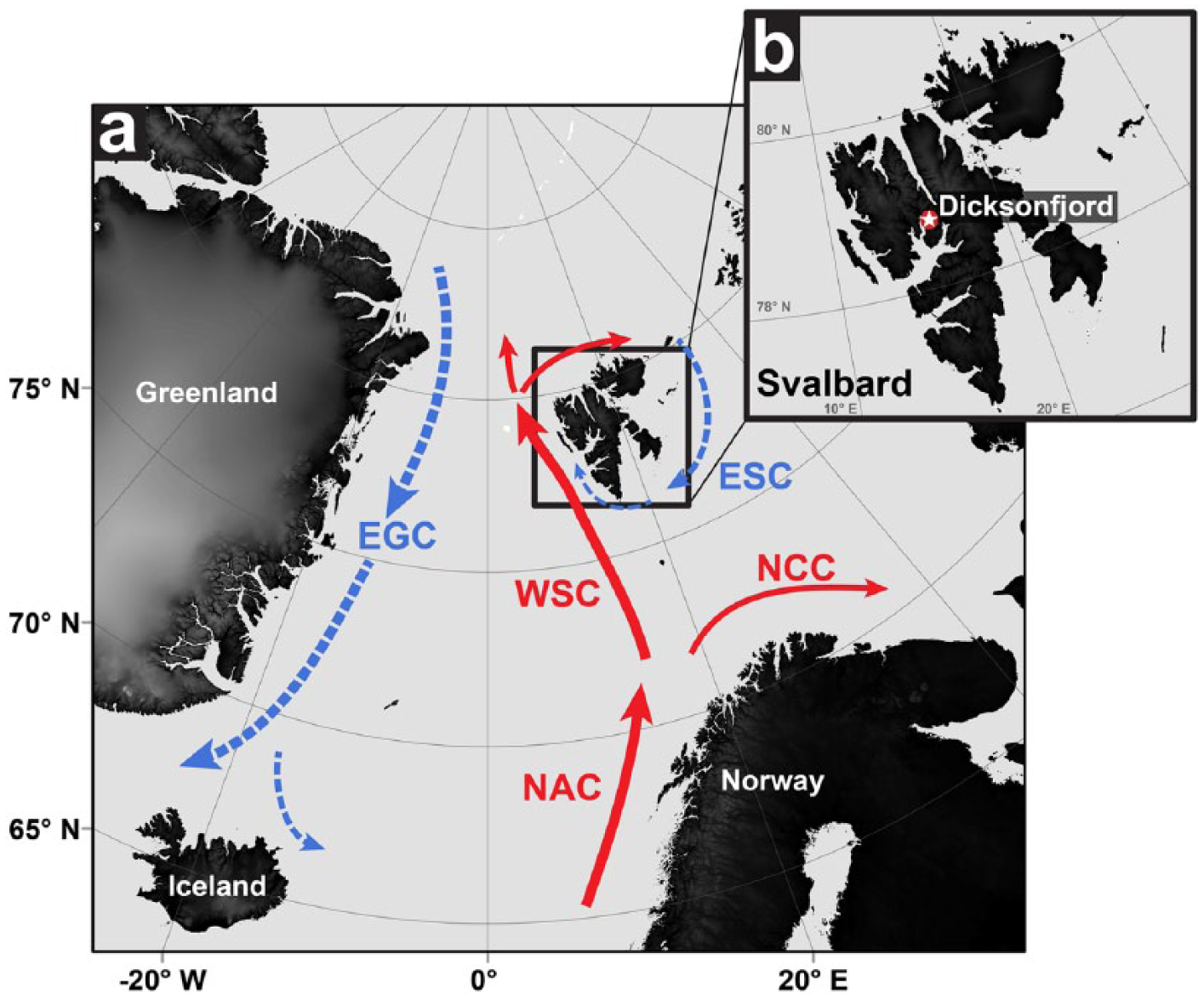
Map of Svalbard and the Nordic Seas showing major ocean currents. (a) Map illustrating the locality of the Svalbard archipelago between the northern North Atlantic Ocean and the Arctic Ocean. Solid arrows indicate the transport of relatively warm and salty water masses northwards, that is, Norwegian Atlantic Current (NAC), Norwegian Coastal Current (NCC) and West Spitsbergen Current (WSC). Dashed arrows indicate southward flows of relatively cold water, that is, East Greenland Current (EGC) and East Spitsbergen Current (ESC). (b) Map of Svalbard indicating the sample locality in Dicksonfjorden (star symbol) of Arctica islandica at about 79°N.

Of the climate proxies available for the Arctic HCO, for example, ice rafted debris (Bond et al., 2001; Hald et al., 2004), benthic and planktonic foraminifera (e.g. Rasmussen et al., 2012), diatoms (e.g. Birks and Koc, 2002; Koc Karpuz and Jansen, 1992) or plant macrofossils (Birks, 1991), most have a very limited temporal resolution (e.g. 10–70 years in ice cores and sediment cores; Bond et al., 2001; Hald et al., 2007; Reusche et al., 2014; Sarnthein et al., 2003). Here, we examine three sub-fossil specimens of the marine bivalve Arctica islandica derived from raised beach deposits (~5 m a.s.l.) at Kapp Nathorst inside Dicksonfjorden (Figure 1b), a side-fjord of Isfjorden, the largest fjord on Spitsbergen (Nilsen et al., 2008). The longevity of A. islandica (more than 500 years; Butler et al., 2013; Ropes and Murawski, 1983; Schöne et al., 2005a), its wide northern boreal distribution as well as its abundance in the fossil record (Dahlgren et al., 2000) qualifies this particular species for palaeo-environmental and palaeo-climatic reconstructions on decadal as well as on sub-annual time scales (Butler et al., 2013; Schöne, 2013; Wanamaker et al., 2011). Previous studies on growth, physiology (e.g. Begum et al., 2010; Morton, 2011) and shell formation (e.g. Stemmer et al., 2013; Witbaard et al., 1999) make A. islandica a well-calibrated and understood high-resolution bio-archive for palaeo-climate studies. This species precipitates its shell carbonate in isotopic equilibrium with ambient seawater (Weidman et al., 1994), and previous studies, for example, by Peacock (1989), Buchardt and Simonarson (2003) and Schöne et al. (2004), have successfully used stable oxygen isotope values (δ¹⁸O_shell) in A. islandica to reconstruct annual and sub-annual water temperatures. However, A. islandica is extinct in modern Svalbard, as mean summer water temperatures of about 5–6°C (see Table 1 for summary) are considerably below the range of about 9–16°C required by this species for successful reproduction and recruitment (Golikov and Scarlato, 1973; Lutz et al., 1982; Peacock, 1989).

Table 1.

Environmental data. Summary of published data on modern maximum and minimum water temperatures for the shelf area and fjords around Svalbard. Information given was used to estimate modern maximum, minimum and average water temperatures as well as the seasonal range for modern bottom water temperatures (BWTs). List does not claim to be complete.

Locality (Svalbard)	Latitude	Max temp. (°C)	Min temp. (°C)	Water mass/depth	Based on	Time	Reference
Hinlopenstretet	80°N	+4–5	–	–	CTD	Summer 1984	Koc et al. (2002)
Kongsfjorden	79°N	+7	−1	Bottom (11 m)	Ferrybox	Jul 2012–Apr 2014	HZG/AWI (http://tsdata.hzg.de)
Kongsfjorden	79°N	+7	−1	9 m (2 m above bottom)	CTD	Jul 2012–Aug 2013	HZG/AWI (http://tsdata.hzg.de)
Kongsfjorden	79°N	+7	−1.8	–	Logger	Sep 2009–May 2011	Laudien (2011)
W Svalbard shelf	79°N	+5–6	+1	0–300 m	CTD	Aug 2005	Rasmussen et al. (2014)
Kongsfjorden	79°N	+7	−1	0–400 m	Mooring/CTD	2000–2003	Cottier et al. (2005)
Kongsfjorden shelf	79°N	+5	−1.5	0–400 m	CTD	Sep 2000, Apr 2002/2007	Tverberg and Nøst (2009)
Kongsfjorden	79/78°N	+3	0	0–50 m	CTD	Jul 2002, Sep 2005	MacLachlan et al. (2007)
W Spitsbergen shelf	79–77°N	+6	–	0–50 m	CTD	Sep 1998, 1999, 2000	Saloranta and Svendsen (2001)
Isfjorden shelf/slope	78°N	+7	−1	0–300 m	CTD	Aug 2002, 2003, 2004	Berge et al. (2005)
Isfjorden shelf	78°N	+7.8	–	–	CTD	Aug 2004	Slubowska-Woldengen et al. (2007)
Dicksonfjorden	78°N	+8	−1.8	0–100 m	CTD	Jul/Aug 2005	Forwick (2005)
W Spitsbergen shelf	78°N	+5	−1	–	CTD	Jul/Aug 1981	Gammelsrød and Rudels (1983)
Billefjorden	78°N	+7	−1.7	0–150 m	Mooring/CTD	Oct 2010–Aug 2011	Christensen (2012)
W Spitsbergen	78°N	+6	+2	0–600 m	–	Oct 2006, Aug 2007	Spielhagen et al. (2011)
Isfjorden shelf	78°N	+3.7	–	Modelled SST	NORA10	Jul–Sep average 1958–2009	Reistad et al. (2011)
Hornsund	77°N	+3	−1.88	Near bottom water	Reverse thermometer	1984/1985	Weslawski et al. (1988)

We measure stable oxygen isotope values (δ¹⁸O_shell) in carbonate sampled with high spatial resolution along the growth trajectory in A. islandica shells to reconstruct temperatures and seasonality during the HCO interval. We present a high-resolution insight into the climatic conditions that may be experienced in the Polar region by the end of the century under current modelling projections and demonstrate the power of this bio-archive for accurate and sub-seasonal environmental reconstructions. We discuss the reliability of these results with respect to possible fluctuations of salinity and associated variations in seawater chemistry (δ¹⁸O_SW), and to changes in ice volume as well as in the length of the growing season.

Material and methods

Shell origin and preparation

Three A. islandica shells were collected during fieldwork (O Salvigsen) in 1991 and were found in life-position in sub-littoral layers in raised beach deposits (about 5 m a.s.l.) at Kapp Nathorst on the eastern shore of Dicksonfjorden (78°46′41″N, 15°24′21″E, Figure 1). The landmasses of most of Svalbard experienced considerable relative uplift during the Holocene because of reduced ice load after the last glacial maximum, and shells of different molluscs are commonly revealed in raised beach deposits following erosion by the sea or small rivers. Sub-fossil specimens of A. islandica appear to be more frequent in Dicksonfjorden than in other localities in Svalbard, particularly at Kapp Nathorst where these specimens were retrieved (cf. Feyling-Hanssen, 1955). This post-glacial uplift has been dated in many places by age determinations of driftwood and whale bones found on these raised beaches (e.g. Bondevik et al., 1995; Forman, 1990; Landvik et al., 1998; Salvigsen and Høgvard, 2006) and a minimum value of 70 m is considered as a safe estimate for the post-glacial marine limit in Dicksonfjorden based on field observations. The depth at which these shells lived during the Holocene is discussed in section ‘Water depth’.

After collection, the shells were air-dried and kept in storage until 2011. Three shells (shell IDs: AI-DiFj-02, AI-DiFj-03 and AI-DiFj-04) were selected for analysis and were externally strengthened with an epoxy resin cover to protect them from breakage. A 5-mm cross-section was prepared by sawing along the line of strongest growth (running perpendicular to the growth lines) using a low-speed precision saw (IsoMet; Buehler) equipped with a 0.4-mm diamond-coated saw blade. Cross-sections were then ground using a manual grinder (Phoenix Alpha; Buehler) and sand paper with three different grain sizes (15, 10 and 5 µm).

Preservation of shell material

When considering geochemical analyses on biogenic fossil and sub-fossil carbonate, a check for diagenetic alteration is a key step. The bivalve A. islandica builds its three shell layers out of aragonite (e.g. Schöne, 2013). Depending on the existence of pressure, heat and/or hydrothermal fluids within the ambient sediment layer, fossil biogenic aragonite may recrystallize to calcite over time (the more stable polymorph of calcium carbonate; e.g. Maliva, 1998), affecting the original isotope signal of the carbonate. All shells in this study have been checked for recrystallization (i.e. from pristine aragonite to calcite), using a confocal Raman microscope (CRM; WITec alpha 300 R; cf. Nehrke et al., 2012), equipped with a diode laser (excitation wavelength 488 nm) and a 20× Zeiss objective. CRM is a non-destructive method and provides a high spatial resolution (a few hundred nanometres). Instrumental settings and procedure follow Nehrke et al. (2012). In each of the three 5-mm shell cross-sections dedicated for stable oxygen isotope analysis, the sampling areas were checked by CRM scans and single spot measurements.

Dating of shell material

All three sub-fossil shells in this study have been radiocarbon dated (Accelerator Mass Spectrometry (AMS) ¹⁴C) at the Poznań Radiocarbon Laboratory in Poland. The periostracum and any adhering sediment were carefully removed from the outer surface of the shells using a hand drill device (Type Proxxon Minimot 40/E) and 50-mg samples of shell carbonate from the ventral margin were taken for analysis. AMS ¹⁴C results were corrected using the program CALIB version 6.1.0 (Stuiver and Reimer, 1993, http://calib.qub.ac.uk/calib/) and the Marine09 calibration curve (Reimer et al., 2009). For Svalbard, a regional reservoir age correction (ΔR) of 93 ± 23 years has been applied, following the descriptions in Slubowska-Woldengen et al. (2007) and Ebbesen et al. (2007).

Stable oxygen isotope analysis (δ¹⁸O)

Carbonate samples were taken from the outer shell layer (Dettman and Lohmann, 1995) using a 700-µm mill bit (Komet/Gebr. Brasseler GmbH & Co. KG) mounted onto an industrial high precision drill (Minimo C121; Minitor Co., Ltd) and attached to a binocular microscope. Two identical consecutive ontogenetic years (i.e. ontogenetic years 10 and 11 in each of the three shells; counted within the internal growth record) have been sampled in each of the three shells to ensure comparability between individuals. The average sample weight for all 796 samples was ~48 µg, while the average spatial sampling resolution was ~50 µm (Table 3).

Measurements were conducted on a Thermo Finnigan MAT 253 isotope ratio mass spectrometer coupled with an automated carbonate preparation device (Kiel IV). Measurements were calibrated against the international NBS-19 standard and reported in δ-notation versus Vienna Peedee Belemnite (VPDB). The long-term precision based on an internal laboratory standard (Solnhofen limestone) measured over a 1-year period together with samples was better than ±0.08‰.

When calculating temperatures from sub-fossil shell carbonate, it is important to consider changes in ice volume over geological time-scales as this affects marine δ¹⁸O_SW values. Based on the work of Fairbanks (1989), δ¹⁸O_shell values were corrected with individual factors (based on their specific radiocarbon ages) for each of the three specimens (Table 3) to make them comparable to modern measurements. Finally, we calculated palaeo-temperatures for all six individual ontogenetic years according to Dettman et al. (1999), which takes into account that the assumed δ¹⁸O_SW value of 0.20‰ as given by MacLachlan et al. (2007) for transformed AW in Kongsfjorden at water depths between 6 and 52 m was reported against Vienna Standard Mean Ocean Water (VSMOW). This δ¹⁸O_SW value is confirmed by a δ¹⁸O_SW value of 0.19‰ measured in water, from close to the mouth of Isfjorden (77.85°N, 11.9°E, T = 3.36°C, S = 34.48 psu) at a water depth of 52.5 m on 6 September 2001 (A Mackensen, unpublished data). For the error estimate, we assume the modern δ¹⁸O_SW variability (based on MacLachlan et al., 2007), which results in uncertainties of 0.87°C (+0.20‰) for highest and 0.61°C (−0.14‰) for lowest temperature estimates, respectively (legend in Figure 4).

Modern water temperature data from Svalbard

Modern long-term measurements of fjord water temperatures at West Spitsbergen are rare. Hence, information from different sources has been combined to obtain reliable estimates of seasonal maximum and minimum water temperatures (Table 1). According to this database, water temperatures below 2-m water depth range between −1°C in winter and 5–6°C in summer.

Results

Preservation of shell material

CRM scans of the shell areas designated for oxygen isotope sampling indicated no traces of calcite. Hence, all shells were considered to be pristine aragonite and thus reliable in terms of radiocarbon dating (AMS ¹⁴C) and stable oxygen isotope analysis (δ¹⁸O).

Dating of shell material

Calibrated radiocarbon (AMS ¹⁴C) ages for the three shell specimens in this study cover a period from 9954–9782 cal. yr BP (Table 2). Therefore, all shells are assigned to the early Holocene (cf. Hald et al., 2004; Kaufman et al., 2004). This is in good agreement with previously published radiocarbon ages for sub-fossil mollusc shells from Svalbard (see Salvigsen, 2002 for summary). Furthermore, two recently reported age determinations of A. islandica shells from Hollendarbukta, outer Isfjorden, revealed ages of 9780 ± 180 (sample ID: Lu-6992) and 9670 ± 80 (sample ID: GIN-14735) cal. yr BP respectively (Sharin et al., 2014).

Table 2.

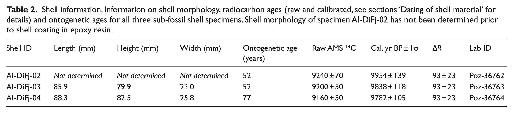
Shell information. Information on shell morphology, radiocarbon ages (raw and calibrated, see sections ‘Dating of shell material’ for details) and ontogenetic ages for all three sub-fossil shell specimens. Shell morphology of specimen AI-DiFj-02 has not been determined prior to shell coating in epoxy resin.

Shell ID	Length (mm)	Height (mm)	Width (mm)	Ontogenetic age (years)	Raw AMS ¹⁴C	Cal. yr BP ± 1σ	ΔR	Lab ID
AI-DiFj-02	Not determined	Not determined	Not determined	52	9240 ± 70	9954 ± 139	93 ± 23	Poz-36762
AI-DiFj-03	85.9	79.9	23.0	52	9200 ± 50	9838 ± 118	93 ± 23	Poz-36763
AI-DiFj-04	88.3	82.5	25.8	77	9160 ± 50	9782 ± 105	93 ± 23	Poz-36764

Stable oxygen isotope analysis (δ¹⁸O)

δ¹⁸O_shell profiles of all studied specimens (AI-DiFj-02, AI-DiFj-03, AI-DiFj-04) show two clear and distinct seasonal cycles (Figure 2). The darker winter bands within the shell carbonate (dashed lines in Figure 2) occur immediately before the most positive δ¹⁸O_shell values (seen in the direction of growth). The δ¹⁸O_shell values range from 1.4‰ to 4.3‰ in specimen AI-DiFj-02, from 1.3‰ to 4.0‰ in specimen AI-DiFj-03 and from 1.0‰ to 3.9‰ in specimen AI-DiFj-04 (Figure 2), that is, they exhibit very similar absolute amplitudes of 2.7‰ to 2.9‰ in all three shells. Detailed information on the spatial sampling resolution as well as individual sample numbers in all six ontogenetic years is given in Table 3.

Figure 2.

δ¹⁸O_shell profiles in six ontogenetic years of A. islandica. Stable oxygen isotope (δ¹⁸O_shell) profiles from three early Holocene A. islandica specimens covering a period of two ontogenetic years each. All three profiles show two distinct annual cycles. Dotted lines indicate darker growth bands in the shell carbonate. d.o.g.: direction of growth. (a) Specimen AI-DiFj-02 with a total of 298 isotope measurements covers a range from 1.4‰ to 4.3‰. (b) Specimen AI-DiFj-03 with a total of 100 isotope measurements covers a range from 1.3‰ to 4.0‰. (c) Specimen AI-DiFj-04 with a total of 398 isotope measurements covers a range from 1.0‰ to 3.9‰.

Table 3.

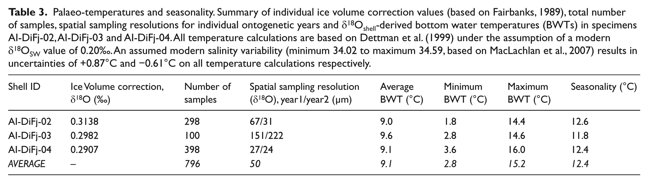
Palaeo-temperatures and seasonality. Summary of individual ice volume correction values (based on Fairbanks, 1989), total number of samples, spatial sampling resolutions for individual ontogenetic years and δ¹⁸O_shell-derived bottom water temperatures (BWTs) in specimens AI-DiFj-02, AI-DiFj-03 and AI-DiFj-04. All temperature calculations are based on Dettman et al. (1999) under the assumption of a modern δ¹⁸O_SW value of 0.20‰. An assumed modern salinity variability (minimum 34.02 to maximum 34.59, based on MacLachlan et al., 2007) results in uncertainties of +0.87°C and −0.61°C on all temperature calculations respectively.

Shell ID	Ice Volume correction, δ¹⁸O (‰)	Number of samples	Spatial sampling resolution (δ¹⁸O), year1/year2 (µm)	Average BWT (°C)	Minimum BWT (°C)	Maximum BWT (°C)	Seasonality (°C)
AI-DiFj-02	0.3138	298	67/31	9.0	1.8	14.4	12.6
AI-DiFj-03	0.2982	100	151/222	9.6	2.8	14.6	11.8
AI-DiFj-04	0.2907	398	27/24	9.1	3.6	16.0	12.4
AVERAGE	–	796	50	9.1	2.8	15.2	12.4

Discussion

Since there is no living modern analogue of Arctica islandica at such high latitudes (79°N) under present climate conditions against which to compare the isotope data, essential aspects concerning the observed δ¹⁸O_shell signal have to be addressed prior to an interpretation. First, we have to determine the time period represented by the analysed shell sections. Next, we need to infer the corresponding water depth, and finally, we have to discuss crucial environmental parameters such as salinity variability and δ¹⁸O_SW values. Only after a cautious evaluation of these issues we will proceed towards reconstructions for water temperatures on seasonal time-scales.

Season of growth

The exact duration of the season of growth, and therefore, the time span of the annual temperature profile of each shell increment recorded during the year, is a crucial, albeit unknown factor for sub-fossil A. islandica. Shell growth depends primarily on water temperature and food availability (e.g. Witbaard et al., 1997). The annual growth line formation in this species occurs in late summer/autumn. However, the exact reasons for the regular slow-down of growth remain enigmatic (Schöne, 2013).

Studies of modern A. islandica populations indicate geographic variability in the duration of the growing season, for example, from February to September in the North Sea (Schöne et al., 2004), from January to August at the New Jersey coast (Jones, 1980) and from May to December near Cape Cod (Weidman et al., 1994). Seasonality in temperature and primary production (i.e. food availability) is predominantly driven by the annual cycle in daylight hours, which is a function of geographical latitude. In the North Sea (54°N), daily light hours range between 7 and 17 h, whereas at Spitsbergen (79°N) the range is 0–24 h, with 4 months total darkness and 4 months 24-h daylight (21 April–21 August) per year. Correspondingly, the productive period is shorter in Spitsbergen (Hop et al., 2002), and hence, the availability of fresh food for this bottom living deposit feeder is limited. Therefore, it is most likely that the season of growth for Holocene A. islandica at Svalbard was shorter than at localities where this species occurs nowadays.

Today, the first phytoplankton bloom at Spitsbergen usually develops in April or May (Christensen, 2012; Wassmann et al., 2006; Weslawski et al., 1988) as sea-ice retreats and light conditions no longer limit growth (Sakshaug et al., 2009). During the early Holocene, however, sea-ice cover was greatly reduced (Svendsen and Mangerud, 1997), most probably causing phytoplankton production to be primarily coupled to sunlight availability. Thus we assume that the main growing season of early Holocene A. islandica at Spitsbergen ranged from approximately April to August, covering at least the period of constant daylight.

Whether this assumed April to August growing season would cover the whole annual temperature amplitude remains uncertain. However, modern maximum water temperatures are observed in July/August (e.g. Christensen, 2012, Table 1). We are therefore confident that the early Holocene shells record the maximum annual temperature. Modern minimum water temperatures of about −2°C to 0°C are measured until May, depending on locality and hydrography (e.g. Christensen, 2012). We therefore assume that the annual Holocene seasonal signal is most likely fully recorded by the A. islandica shells, although minimum winter temperatures are possibly truncated.

Water depth

For the palaeo-environmental reconstruction, it is crucial to know the water depth from which the observed signals are derived, as this affects mean annual temperature and the degree of seasonality experienced by the organisms. We cannot determine directly whether Holocene A. islandica specimens lived above or below the thermocline and hence must rely on assumptions based on modern observations.

It is possible to estimate a minimum water depth value for the dated A. islandica shells at Kapp Nathorst based on the analysis of a whale cranium, which was radiocarbon dated to an age of 8825 ± 105 yr BP (sample ID: T-17118; Borge et al., 2007) and was found at 25 m a.s.l. at Kapp Smith, on the western side of Dicksonfjorden. The following considerations and estimations are based mainly on the isobase pattern of Holocene shoreline as shown in Salvigsen (1984), Bondevik et al. (1995) and Landvik et al. (1998). The 25-m level of the whale cranium at Kapp Smith corresponds to an approximately 5-m higher level at Kapp Nathorst because the shoreline height rises east to west across Dicksonfjorden. The age difference between our dated A. islandica shells at Kapp Nathorst (Table 2) and the whale cranium at Kapp Smith is approximately 400 years. In Billefjorden (the adjacent fjord to Dicksonfjorden), the average uplift between 10,000 and 8000 yr BP is estimated to 1.9 m per century (Salvigsen, 1984), equivalent to 7.6 m during 400 years. We therefore consider it reasonable to add an additional 5 m of uplift to Dicksonfjorden. Thus, the expected height from the contemporaneous shoreline to our A. islandica shells is reasoned to be at least 35 m a.s.l. As the shells at Kapp Nathorst were in fact found at approximately 5 m a.s.l., we therefore conclude that the water depth at which these specimens lived was at least 30 m.

Estimating the seasonal thermocline depth remains challenging. Modern long-term data on the temperature structure of different water columns in Spitsbergen fjords are scarce. MacLachlan et al. (2007) describe the thermocline at Kongsfjorden to be situated at approximately 5-m water depth in September. In Dicksonfjorden, in August 2005 (Forwick, 2005) the uppermost water body, which was characterized by low salinities due to meltwater influx, extended to 10- to 20-m water depth. Even though water column stratification varies seasonally and between fjords, it appears to be a common feature of Svalbard coastal waters in summer. According to Rasmussen et al. (2014), a strong pycnocline existed in the West Svalbard shelf area (79°N) before 9600 yr BP, which argues for a stratified water column dominated by AW at the bottom. Reduced or even absent glaciers and sea-ice (e.g. Svendsen and Mangerud, 1997) resulted in reduced meltwater and freshwater influx, which led to an entirely AW occupied water column on the shelf between ca. 9000 and 6000 yr BP (Rasmussen et al., 2014). Both scenarios would have led to much lower salinity fluctuations in bottom waters and more pronounced water column stratification during Holocene summer conditions at Spitsbergen (Hald et al., 2007; Rasmussen et al., 2012). Hence, we assume that during the early Holocene, the water column in Dicksonfjorden remained stratified for the duration of the growing season (April to August) with a thermocline situated between 0- and 15-m water depths.

Previous studies have discussed seasonal oxygen isotope profiles in mollusc shells (e.g. Arthur et al., 1983; Purton and Brasier, 1997; Williams et al., 1982) or fish otolith (e.g. Ivany et al., 2000) in respect to stratification, growth and/or temperature. According to Schöne and Fiebig (2009), oxygen isotope profiles derived from shelf areas can indirectly indicate whether a bivalve lived above or below the thermocline. A saw-toothed shaped profile argues for a position below the thermocline, with rather stable conditions interrupted by ‘sudden’ major winter mixing events. A more sinusoidal profile pattern argues for a position above or close to the thermocline, as the water temperatures above the thermocline would have experienced greater seasonality.

In this study, isotope profiles of specimens AI-DiFj-02 and AI-DiFj-03 exhibit plateau-like intervals that are interjected by positive peaks in δ¹⁸O_shell values (Figure 2a and b). This pattern indicates stable temperature and salinity conditions for most of the growing season, which are interrupted by deeper seasonal mixing. The δ¹⁸O_shell profile of AI-DiFj-04 exhibits a more sinusoidal pattern but has the same range of δ¹⁸O_shell values as the other two specimens (Figure 2c). However, the degree of consistency in δ¹⁸O_shell values through an extraordinarily high sample density of 398 single samples in AI-DiFj-04 strongly argues against a life above the thermocline in a fjord setting. Furthermore, specimen AI-DiFj-04 recorded the warmest winter temperatures (3.6°C) of all three specimens. Presumably, the three specimens lived at slightly different geological times throughout the early Holocene (Table 2), and hence they may have inhabited slightly different water depths relative to the position of the thermocline. Therefore, the differences in the AI-DiFj-04 isotope profile might be explained by a vertical displacement of the seasonal thermocline (Schöne et al., 2005b). It should also be noted that Schöne and Fiebig (2009) describe isotope profiles for mid-latitude shelf area conditions, which are only of limited applicability to a high Arctic fjord setting such as Svalbard.

Although the interpretation of oxygen isotope profiles is not unambiguous and could be explained by several combinations of stratification, temperature and/or growth, we are confident to conclude that a living depth of at least 30 m b.s.l. for these sub-fossil A. islandica specimens from Spitsbergen would have been below the seasonal thermocline during the Holocene at this fjord.

(Sub-annual) salinity changes and δ¹⁸O_SW

Temperature reconstructions based on δ¹⁸O_shell values should be interpreted with caution, as δ¹⁸O_SW values at the time of shell formation can vary on geological (ice volume) and sub-annual (seasonal) time-scales with changes in water temperature and salinity (Jansen, 1989; MacLachlan et al., 2007). To account for the effect on δ¹⁸O_SW of less global ice volume during the early Holocene, we applied correction values to δ¹⁸O_shell based on the work of Fairbanks (1989; Table 3). Sub-annual changes in salinity during the early Holocene in Spitsbergen fjords have not been determined thus far, but might have influenced δ¹⁸O_SW values. Our salinity and temperature estimates are therefore based on two assumptions.

The correlation between salinity and δ¹⁸O_SW is nearly linear and latitude dependent (e.g. Azetsu-Scott and Tan, 1997; Mikalsen and Sejrup, 2000). For Spitsbergen, MacLachlan et al. (2007) established this correlation from modern annual δ¹⁸O_SW values and salinity data for Kongsfjorden, a fjord north of Isfjorden on the west coast of Spitsbergen, whose hydrology is considered to be similar to Isfjorden (Rasmussen et al., 2012). This allows the conversion of salinity measurements from fjords on Spitsbergen into δ¹⁸O_SW values. Accordingly, we assume a δ¹⁸O_SW value of 0.20‰ (ranging from 0.06‰ to 0.40‰) in our calculations. This is suggested by MacLachlan et al. (2007) for the outer fjord transformed AW at a depth of 6–52 m, the water mass that is considered most likely to resemble early Holocene, glacier-reduced water conditions. We assume the same annual salinity range of Kongsfjorden (from 34.02 to 34.59) for the early Holocene Dicksonfjorden to provide an error estimate for our temperature reconstructions (Figure 4). Additional average δ¹⁸O_SW values given in MacLachlan et al. (2007) for the inner fjord deep water (>2 m) of 0.10‰ and outer fjord AW (76–354 m) of 0.24‰ result in consistently increased (by 0.17°C for δ¹⁸O_SW = 0.24‰) or decreased (by 0.43°C for δ¹⁸O_SW = 0.10‰) water temperature values, both having comparable salinity ranges (0.7 for δ¹⁸O_SW = 0.10‰ and 0.48 for δ¹⁸O_SW = 0.24‰) and therefore not having an impact on the key findings in this study.

During modern times and during the early Holocene, fjords along the west coast of Spitsbergen have strongly been influenced by the impact of AW, derived from the WSC (Berge et al., 2005; Peacock, 1989; Salvigsen, 2002; Salvigsen et al., 1992). On the western shelf of Svalbard (79°N), the development of a strong pycnocline in late spring separates low-salinity surface water caused by meltwater influx from the warmer and more saline AW beneath (Rasmussen et al., 2014). Consequently, the influence of AW on bottom waters of Isfjorden would have been strongest during the summer growing season of A. islandica (see section ‘Season of growth’, Rasmussen et al., 2007, 2012; Skirbekk et al., 2010; Slubowska et al., 2005; Slubowska-Woldengen et al., 2007). Although the modern hydrological summer conditions at Isfjorden are considered to be relatively stable (Berge et al., 2005), conditions during the early Holocene are presumed to have been even less variable (Ebbesen et al., 2007). Due to greatly reduced extent of glaciers and sea-ice (Salvigsen, 2002; Svendsen and Mangerud, 1997), pronounced water column stratification (Rasmussen et al., 2014) and a much enhanced WSC (Hald et al., 2004; Sarnthein et al., 2003), subsurface AW had a more distinct influence at the bottom than present (Hald et al., 2004; Koc and Jansen, 2002; Rasmussen et al., 2014). Therefore, applying the modern salinity variability of 34.02–34.59 to the early Holocene (ca. 9850 cal. yr BP) will likely overestimate Holocene variability in water chemistry. Our considerations imply that the benthos below 30-m water depth has been exposed to AW primarily, derived from the WSC. Consequently, we follow Lubinski et al. (2001) and Rasmussen et al. (2012) in expecting that Holocene benthic δ¹⁸O_shell values from the west coast of Spitsbergen will reflect variations in temperature rather than in salinity.

Palaeo-temperatures and seasonality

We present the first high temporal resolution snapshot of palaeo-temperature and seasonality at ⩾30-m water depth in an Arctic fjord setting during HCO. Due to the above-mentioned uncertainties in growing season, water depth, absolute δ¹⁸O_SW values and sub-annual salinity variability (see also sections ‘Stable oxygen isotope analysis (δ¹⁸O)’), the reconstructed temperatures are associated with a certain error. Nevertheless, they correspond very well with the preferred temperature range of modern A. islandica (Golikov and Scarlato, 1973; Witbaard et al., 1997), which is known to tolerate temperatures from about 20°C down to 1°C (Cargnelli et al., 1999) and occasionally below 0°C (Peacock, 1989). However, A. islandica growth may have paused during winter, and thus the shell may have not recorded the true ambient minimum temperature.

The average minimum bottom water temperature (BWT) recorded is 2.8°C and thus about 4°C higher than modern minimum winter temperatures (Figure 3, Table 3). Furthermore, the maximum BWT amounts to 15.2°C, which is 8–10°C higher than modern maximum summer BWTs in this region (Figure 3, Table 3). Maximum BWTs represent peak values, occurring during the first half of the growing season in all six ontogenetic years (Figure 4). This might be due to a down-mixing of low-salinity surface waters (associated with more negative δ¹⁸O_SW values) during thermocline formation at the beginning of the growing season. On the other hand, maximum BWTs in inner fjords may be higher in general compared with shelf regions, owing to ‘… atmospheric heating in sheltered areas and small inflow of cold water …’ (Salvigsen et al., 1992). The early Holocene was associated with an 8% increased summer insolation (ACIA, 2004; Berger and Loutre, 1991; Koc et al., 1993), which may have caused stronger heating of the fjords during summer. Furthermore, glaciers, sea-ice and cold Arctic water influx were largely reduced compared with today (Reusche et al., 2014; Salvigsen, 2002; Sarnthein et al., 2003), and due to an increased WSC, warmer AW dominated subsurface waters on the shelf (Hald et al., 2004; Rasmussen et al., 2014) and therefore most probably also the hydrology inside Isfjorden/Dicksonfjorden.

Figure 3.

Reconstructed bottom water temperatures (BWTs) and seasonality. Temperatures derived from stable oxygen isotope values (δ¹⁸O_shell) of six individual ontogenetic years of specimens AI-DiFj-02, AI-DiFj-03 and AI-DiFj-04 (see Figure 2). Values have been individually corrected for ice volume changes (Table 3) and a modern δ¹⁸O_SW value of 0.20‰ has been assumed. Individual years are given as box-and-whisker plots with box giving the first quartile, median and third quartile (horizontal lines from top to bottom). Upper and lower whiskers give maximum and minimum of all data. Reconstructed early Holocene BWTs represent average values based on all six ontogenetic years (Table 3). Modern BWTs are based on references in Table 1.

Figure 4.

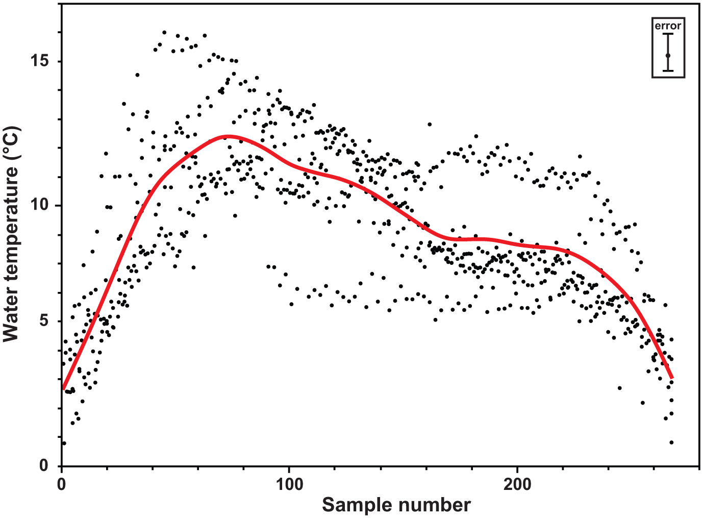
Seasonal temperature curve. Reconstructed water temperature based on all 796 stable oxygen isotope measurements. Spacing between individual data points has been adjusted to cover identical temporal ranges in all six ontogenetic years. Average line has been calculated using a cubic spline (λ = 8000; statistical software JMP version 9.0.1; SAS Institute Inc., 2007). Error bar in inlay accounts for uncertainty due to modern seasonal salinity variation and applies for all single data points (see section ‘Stable oxygen isotope analysis (δ¹⁸O)’).

Average BWT across all samples is 9.1°C, varying by ±0.3°C among the three specimens (Table 3). Since there are no long-term records of Dicksonfjorden water temperature, a direct modern analogue for comparison is lacking. A compilation of temperature data from a wider area (Table 1) indicates modern average water temperature of about 3°C at comparable water depth, which would indicate a decline in BWTs of about 6°C since the HCO. Furthermore, an average BWT of about 9°C satisfies the assumption that 9–10°C is the required summer minimum water temperature needed for spawning and reproduction in A. islandica (Golikov and Scarlato, 1973; Lutz et al., 1982; Peacock, 1989). All three shell specimens in this study recorded almost identical seasonal temperature amplitudes of 12.4°C (±0.4°C; Figures 3 and 4, Table 3). Modern water temperatures at comparable depth (Table 1) range between −1°C and 5°C, that is, the seasonal amplitude is about 6°C. Hence, average temperature has declined by 6°C since the HCO, and the seasonal amplitude has narrowed by 50%.

Even though the HCO period did not occur simultaneously throughout the Nordic Sea and Barents Sea areas, the 6°C higher HCO temperature found here is in very good agreement with previous temperature reconstructions for the northern North Atlantic HCO derived from diatoms (+3–5°C in Birks and Koc, 2002) and foraminifera (+4–5°C in Sarnthein et al., 2003; +6°C in Hald et al., 2004; +6°C in Ebbesen et al., 2007; +3–4°C in Rasmussen et al., 2014; and up to +6°C for BWT based on oxygen isotope data) in sediment cores. Additionally, studies based on plant macrofossils (‘at least’ 1.5°C higher July air temperatures in Birks, 1991), mollusc shells (+4°C in Lubinski et al., 1999; based on the work of Salvigsen et al., 1992) and insect data (+4–5°C summer air temperatures in Wohlfarth et al., 1995) support our findings. The reconstructed temperatures and seasonal temperature range presented here correspond very well (±0.1°C) to A. islandica derived southern North Sea water temperature values for the period 1884–1983 given in Schöne et al. (2004), where minimum temperatures of 2.9°C and maximum temperatures of 15.1°C result in a seasonal signal (February to September) of 12.2°C, which was also in good agreement with observational SST data. This suggests that recent southern North Sea conditions may be comparable to HCO conditions at Spitsbergen.

Given this substantiation, our results support the common assertion of polar region amplification associated with global warming (e.g. Hald et al., 2007; Serreze and Francis, 2006; Spielhagen et al., 2011) and the significant difference between global average values and actual regional impacts. Therefore, the presented temperatures might give an indication how an average increase in global temperatures by about 3.7°C, as suggested by the IPCC (2013) report, may be amplified on a regional scale such as the Svalbard archipelago.

Conclusion

We present a palaeo-environmental reconstruction for the early Holocene period in Svalbard, based on three sub-fossil shells of A. islandica from Dicksonfjorden (Figure 1). Radiocarbon (AMS) dating has determined that these specimens lived during the early Holocene Climate Optimum (9954–9782 cal. yr BP, Table 2).

Stable oxygen isotope (δ¹⁸O_shell) profiles of six ontogenetic years from three shells show distinct seasonal patterns with amplitudes of 2.7‰ to 2.9‰ (Figure 2).

Reconstructed maximum and minimum temperatures for the assumed shell growth period (April to August) of 15.2°C and 2.8°C imply a seasonality of about 12.4°C for the early Holocene at Svalbard, giving a first unique palaeo-environmental description of a fjord setting during the Holocene Climate Optimum at Spitsbergen and coinciding with temperature requirements for A. islandica today (Table 3, Figures 3 and 4).

An average BWT of 9.1°C argues for a +6°C warmer HCO at Spitsbergen, and hence our results distinctly exceed most previous global estimates (+1–3°C) but confirm studies indicating an amplified effect (+4–6°C) at high northern latitudes.

Climate archives with a sub-annual temporal resolution at high latitudes in the northern North Atlantic realm are rare. Due to changing climatic conditions over geological time-scales and related changes in the bio-geographic distribution of suitable archive species, it is challenging to provide continuous master chronologies for time spans such as the entire Holocene. However, this study demonstrates the potential of individual shell chronologies as well as of prospective cross-dated floating chronologies of the well-calibrated bio-archive A. islandica for providing valuable insights into palaeoceanographic and palaeo-environmental conditions at single points in time. However, special care has to be taken when interpreting these results as a proxy for the mean climate state of the early Holocene.

Footnotes

Acknowledgements

Kerstin Beyer and Lisa Schönborn (both Alfred Wegener Institute (AWI)) are thanked for their help with the isotope measurements. Further thanks go to Gernot Nehrke (AWI) for help with the Raman microscope and Rosie Sheward (NOC, Southampton) for suggestions that improved the written quality of the manuscript.

Funding

The first author (LB) was financed by the ‘Earth System Science Research School (ESSReS)’, an initiative of the Helmholtz Association of German Research Centres (HGF) at the Alfred Wegener Institute (AWI), Helmholtz Centre for Polar and Marine Research.

References

ACIA (2004) Impacts of a Warming Arctic – Arctic Climate Impact Assessment. Cambridge: Cambridge University Press.

Arthur

Williams

Jones

(1983) Seasonal temperature-salinity changes and thermocline development in the mid-Atlantic Bight as recorded by the isotopic composition of bivalves. Geology 11: 655–659.

Azetsu-Scott

Tan

(1997) Oxygen isotope studies from Iceland to an East Greenland Fjord: Behaviour of glacial meltwater plume. Marine Chemistry 56: 239–251.

Begum

Basova

Heilmayer

. (2010) Growth and energy budget models of the bivalve Arctica islandica at six different sites in the Northeast Atlantic realm. Journal of Shellfish Research 29: 107–115.

Berge

Johnsen

Nilsen

. (2005) Ocean temperature oscillations enable reappearance of blue mussels Mytilus edulis in Svalbard after a 1000 year absence. Marine Ecology Progress Series 303: 167–175.

Berger

Loutre

(1991) Insolation values for the climate of the last 10 million years. Quaternary Science Reviews 10: 297–317.

Birks

CJA

Koc

(2002) A high-resolution diatom record of late-Quaternary sea-surface temperatures and oceanographic conditions from the eastern Norwegian Sea. Boreas 31: 323–344.

Birks

(1991) Holocene vegetational history and climatic change in west Spitsbergen – Plant macrofossils from Skardtjørna, an Arctic lake. The Holocene 1: 209–218.

Bond

Kromer

Beer

. (2001) Persistent solar influence on North Atlantic climate during the Holocene. Science 294: 2130–2136.

10.

Bondevik

Mangerud

Ronnert

. (1995) Postglacial sea-level history of Edgeøya and Barentsøya, eastern Svalbard. Polar Research 14: 153–180.

11.

Borge

Bachmann

Bjørnstad

. (2007) Genetic variation in Holocene bowhead whales from Svalbard. Molecular Ecology 16: 2223–2235.

12.

Buchardt

Simonarson

(2003) Isotope palaeotemperatures from the Tjörnes beds in Iceland: Evidence of Pliocene cooling. Palaeogeography, Palaeoclimatology, Palaeoecology 189: 71–95.

13.

Butler

Wanamaker

Jr Scourse

. (2013) Variability of marine climate on the North Icelandic Shelf in a 1357-year proxy archive based on growth increments in the bivalve Arctica islandica. Palaeogeography, Palaeoclimatology, Palaeoecology 373: 141–151.

14.

Cargnelli

Griesbach

Packer

. (1999) Essential fish habitat source document: Ocean quahog, Arctica islandica, life history and habitat characteristics. NOAA Technical Memorandum 148: 1–12.

15.

Christensen

(2012) Temporal variation of arctic marine picophytoplankton focusing on. Micromonas pusilla (Mamiellophyceae). Master Thesis, University of Oslo.

16.

Cottier

Tverberg

Inall

. (2005) Water mass modification in an Arctic fjord through cross-shelf exchange: The seasonal hydrography of Kongsfjorden, Svalbard. Journal of Geophysical Research 110: C12005.

17.

Dahlgren

Weinberg

Halanych

(2000) Phylogeography of the ocean quahog (Arctica islandica): Influences of paleoclimate on genetic diversity and species range. Marine Biology 137: 487–495.

18.

Dettman

Lohmann

(1995) Microsampling carbonates for stable isotope and minor element analysis: Physical separation of samples on a 20 micrometer scale. Journal of Sedimentary Research, Section A: Sedimentary Petrology and Processes 65: 566–569.

19.

Dettman

Reische

Lohmann

(1999) Controls on the stable isotope composition of seasonal growth bands in aragonitic fresh-water bivalves (unionidae). Geochimica et Cosmochimica Acta 63: 1049–1057.

20.

Ebbesen

Hald

Eplet

(2007) Lateglacial and early Holocene climatic oscillations on the western Svalbard margin, European Arctic. Quaternary Science Reviews 26: 1999–2011.

21.

Fairbanks

(1989) A 17,000-year glacio-eustatic sea level record: Influence of glacial melting rates on the Younger Dryas event and deep-ocean circulation. Nature 342: 637–642.

22.

Feyling-Hanssen

(1955) Stratigraphy of the marine late-Pleistocene of Billefjorden, Vestspitsbergen. Norsk Polarinstitutt Skrifter 107: 1–207.

23.

Forman

(1990) Post-glacial relative sea-level history of northwestern Spitsbergen, Svalbard. Geological Society of America Bulletin 102: 1580–1590.

24.

Forwick

(2005) Marine-Geological Cruise to West Spitsbergen Fjords. Cruise Report, University of Tromsø, Norway, R/V Jan Mayen, 29 July–2 August.

25.

Gammelsrød

Rudels

(1983) Hydrographic and current measurements in the Fram Strait, August 1981. Polar Research 1: 115–126.

26.

Golikov

Scarlato

(1973) Method for indirectly defining optimum temperatures of inhabitancy for marine cold-blooded animals. Marine Biology 20: 1–5.

27.

Hald

Andersson

Ebbesen

. (2007) Variations in temperature and extent of Atlantic Water in the northern North Atlantic during the Holocene. Quaternary Science Reviews 26: 3423–3440.

28.

Hald

Ebbesen

Forwick

. (2004) Holocene paleoceanography and glacial history of the West Spitsbergen area, Euro-Arctic margin. Quaternary Science Reviews 23: 2075–2088.

29.

Hop

Pearson

Hegseth

. (2002) The marine ecosystem of Kongsfjorden, Svalbard. Polar Research 21: 167–208.

30.

Intergovernmental Panel on Climate Change (IPCC) (2013) Climate Change 2013: The Physical Science Basis. Contribution of Working Group I to the Fifth Assessment Report of the Intergovernmental Panel on Climate Change. Cambridge University Press, Cambridge.

31.

Ivany

Patterson

Lohmann

(2000) Cooler winters as a possible cause of mass extinctions at the Eocene/Oligocene boundary. Nature 407: 887–890.

32.

Jansen

(1989) The use of stable oxygen and carbon isotope stratigraphy as a dating tool. Quaternary International 1: 151–166.

33.

Jones

(1980) Annual cycle of shell growth increment formation in two continental shelf bivalves and its paleoecologic significance. Paleobiology 6: 331–340.

34.

Kaufman

Ager

Anderson

. (2004) Holocene thermal maximum in the western Arctic (0–180°W). Quaternary Science Reviews 23: 529–560.

35.

Koc Karpuz

Jansen

(1992) A high-resolution diatom record of the last deglaciation from the SE Norwegian Sea: Documentation of rapid climatic changes. Paleoceanography 7: 499–520.

36.

Koc

Jansen

(2002) Holocene climate evolution of the North Atlantic ocean and the Nordic Seas – A synthesis of new results. In: Wefer

Berger

Behre

. (eds) Climate Development and History of the North Atlantic Realm. Berlin, Heidelberg: Springer, pp. 165–173.

37.

Koc

Jansen

Haflidason

(1993) Paleoceanographic reconstructions of surface ocean conditions in the Greenland, Iceland and Norwegian seas through the last 14 ka based on diatoms. Quaternary Science Reviews 12: 115–140.

38.

Koc

Klitgaard-Kristensen

Hasle

. (2002) Late glacial palaeoceanography of Hinlopen Strait, northern Svalbard. Polar Research 21: 307–314.

39.

Kutzbach

Guetter

(1986) The influence of changing orbital parameters and surface boundary conditions on climate simulations for the past 18,000 years. Journal of the Atmospheric Sciences 43: 1726–1759.

40.

Landvik

Bondevik

Elverhøi

. (1998) The last glacial maximum of Svalbard and the Barents Sea area: Ice sheet extent and configuration. Quaternary Science Reviews 17: 43–75.

41.

Laudien

(2011) Physical Oceanography at Time Series Station Brandal in the Kongsfjorden (Spitsbergen, Arctic), 2009–09 to 2011–06. Bremerhaven: Alfred Wegener Institute, Helmholtz Centre for Polar and Marine Research.

42.

Lubinski

Forman

Miller

(1999) Holocene glacier and climate fluctuations on Franz Josef Land, Arctic Russia, 80°N. Quaternary Science Reviews 18: 85–108.

43.

Lubinski

Polyak

Forman

(2001) Freshwater and Atlantic water inflows to the deep northern Barents and Kara seas since ca 13 ¹⁴C ka: Foraminifera and stable isotopes. Quaternary Science Reviews 20: 1851–1879.

44.

Lutz

Mann

Goodsell

. (1982) Larval and early post-larval development of Arctica islandica. Journal of the Marine Biological Association of the United Kingdom 62: 745–769.

45.

MacLachlan

Cottier

Austin

WEN

. (2007) The salinity: δ¹⁸O water relationship in Kongsfjorden, western Spitsbergen. Polar Research 26: 160–167.

46.

Maliva

(1998) Skeletal aragonite neomorphism – Quantitative modelling of a two-water diagenetic system. Sedimentary Geology 121: 179–190.

47.

Mikalsen

Sejrup

(2000) Oxygen isotope composition of fjord and river water in the Sognefjorden drainage area, Western Norway. Implications for paleoclimate studies. Estuarine, Coastal and Shelf Science 50: 441–448.

48.

Morton

(2011) The biology and functional morphology of Arctica islandica (Bivalvia: Arcticidae): A gerontophilic living fossil. Marine Biology Research 7: 540–553.

49.

Nehrke

Poigner

Wilhelms-Dick

. (2012) Coexistence of three calcium carbonate polymorphs in the shell of the Antarctic clam Laternula elliptica. Geochemistry Geophysics Geosystems 13: Q05014.

50.

Nilsen

Cottier

Skogseth

. (2008) Fjord-shelf exchanges controlled by ice and brine production: The interannual variation of Atlantic Water in Isfjorden, Svalbard. Continental Shelf Research 28: 1838–1853.

51.

Peacock

(1989) Marine molluscs and late quaternary environmental studies with particular reference to the late-glacial period in Northwest Europe: A review. Quaternary Science Reviews 8: 179–192.

52.

Purton

LMA

Brasier

(1997) Gastropod carbonate δ¹⁸O and δ¹³C values record strong seasonal productivity and stratification shifts during the late Eocene in England. Geology 25: 871–874.

53.

Rasmussen

Forwick

Mackensen

(2012) Reconstruction of inflow of Atlantic Water to Isfjorden, Svalbard during the Holocene: Correlation to climate and seasonality. Marine Micropaleontology 94–95: 80–90.

54.

Rasmussen

Thomsen

Skirbekk

. (2014) Spatial and temporal distribution of Holocene temperature maxima in the northern Nordic seas: Interplay of Atlantic-, Arctic- and polar water masses. Quaternary Science Reviews 92: 280–291.

55.

Rasmussen

Thomsen

Slubowska

. (2007) Paleoceanographic evolution of the SW Svalbard margin (76°N) since 20,000 ¹⁴C yr BP. Quaternary Research 67: 100–114.

56.

Reimer

Baillie

MGL

Bard

. (2009) IntCal09 and Marine09 radiocarbon age calibration curves, 0–50,000 years cal BP. Radiocarbon 51: 1111–1150.

57.

Reistad

Breivik

Dinessen

(2011) Ice, Icing and Temperature Conditions around Svalbard. Norwegian Meteorological Institute met.no report 6, pp. 1–82. Available at: http://www.met.no/filestore/report6_2011.pdf.

58.

Reusche

Winsor

Carlson

. (2014) ¹⁰Be surface exposure ages on the late-Pleistocene and Holocene history of Linnébreen on Svalbard. Quaternary Science Reviews 89: 5–12.

59.

Ropes

Murawski

(1983) Maximum shell length and longevity in ocean quahogs, Arctica islandica Linné. International Council for the Exploration of the Sea C.M K 32: 1–8.

60.

Sakshaug

Johnsen

Volent

(2009) Light. In: Sakshaug

(ed.) Ecosystem Barents Sea. Trondheim: Tapir Academic Press, pp. 117–138.

61.

Saloranta

Svendsen

(2001) Across the Arctic front west of Spitsbergen: High-resolution CTD sections from 1998–2000. Polar Research 20: 177–184.

62.

Salvigsen

(1984) Occurrence of pumice on raised beaches and Holocene shoreline displacement in the inner Isfjorden area, Svalbard. Polar Research 2: 107–113.

63.

Salvigsen

(2002) Radiocarbon-dated Mytilus edulis and Modiolus modiolus from northern Svalbard: Climatic implications. Norwegian Journal of Geography 56: 56–61.

64.

Salvigsen

Høgvard

(2006) Glacial history, Holocene shoreline displacement and palaeoclimate based on radiocarbon ages in the area of Bockfjorden, north-western Spitsbergen, Svalbard. Polar Research 25: 15–24.

65.

Salvigsen

Forman

Miller

(1992) Thermophilous molluscs on Svalbard during the Holocene and their paleoclimatic implications. Polar Research 11: 1–10.

66.

Sarnthein

Van Kreveld

Erlenkeuser

. (2003) Centennial-to-millennial-scale periodicities of Holocene climate and sediment injections off the western Barents shelf, 75°N. Boreas 32: 447–461.

67.

Schöne

(2013) Arctica islandica (Bivalvia): A unique paleoenvironmental archive of the northern North Atlantic Ocean. Global and Planetary Change 111: 199–225.

68.

Schöne

Fiebig

(2009) Seasonality in the North Sea during the Allerød and Late Medieval Climate Optimum using bivalve sclerochronology. International Journal of Earth Sciences 98: 83–98.

69.

Schöne

Fiebig

Pfeiffer

. (2005a) Climate records from a bivalved Methuselah (Arctica islandica, Mollusca; Iceland). Palaeogeography, Palaeoclimatology, Palaeoecology 228: 130–148.

70.

Schöne

Freyre

Castro AD

Fiebig

. (2004) Sea surface water temperatures over the period 1884–1983 reconstructed from oxygen isotope ratios of a bivalve mollusk shell (Arctica islandica, southern North Sea). Palaeogeography, Palaeoclimatology, Palaeoecology 212: 215–232.

71.

Schöne

Houk

Freyre

Castro AD

. (2005b) Daily growth rates in shells of Arctica islandica: Assessing sub-seasonal environmental controls on a long-lived bivalve mollusk. PALAIOS 20: 78–92.

72.

Serreze

Francis

(2006) The Arctic on the fast track of change. Weather 61: 65–69.

73.

Sharin

Kokin

Gusev

. (2014) New geochronological data from Quaternary sediments of the Nordenskiold Land area (the Spitsbergen Archipelago). Vestnik St. Petersburg State University Series 7(1): 159–168.

74.

Skirbekk

Kristensen

Rasmussen

. (2010) Holocene climate variations at the entrance to a warm Arctic fjord: Evidence from Kongsfjorden trough, Svalbard. Geological Society, London, Special Publications 344: 289–304.

75.

Slubowska

Koc

Rasmussen

. (2005) Changes in the flow of Atlantic water into the Arctic Ocean since the last deglaciation: Evidence from the northern Svalbard continental margin, 80°N. Paleoceanography 20: PA4014.

76.

Slubowska-Woldengen

Rasmussen

Koc

. (2007) Advection of Atlantic Water to the western and northern Svalbard shelf since 17,500 cal yr BP. Quaternary Science Reviews 26: 463–478.

77.

Spielhagen

Werner

Sorensen

. (2011) Enhanced modern heat transfer to the Arctic by warm Atlantic water. Science 331: 450–453.

78.

Stemmer

Nehrke

Brey

(2013) Elevated CO₂ Levels do not affect the shell structure of the bivalve Arctica islandica from the Western Baltic. PLos One 8: e70106.

79.

Stuiver

Reimer

(1993) Extended ¹⁴C data base and revised CALIB 3.0 ¹⁴C age calibration program. Radiocarbon 35: 215–230.

80.

Svendsen

Mangerud

(1997) Holocene glacial and climatic variations on Spitsbergen, Svalbard. The Holocene 7: 45–57.

81.

Tverberg

Nøst

(2009) Eddy overturning across a shelf edge front: Kongsfjorden, west Spitsbergen. Journal of Geophysical Research 114: C04024.

82.

Wanamaker

Jr Kreutz

Schöne

. (2011) Gulf of Maine shells reveal changes in seawater temperature seasonality during the Medieval Climate Anomaly and the Little Ice Age. Palaeogeography, Palaeoclimatology, Palaeoecology 302: 43–51.

83.

Wassmann

Reigstad

Haug

. (2006) Food webs and carbon flux in the Barents Sea. Progress in Oceanography 71: 232–287.

84.

Weidman

Jones

Lohmann

(1994) The long-lived mollusc Arctica islandica: A new paleoceanographic tool for the reconstruction of bottom temperatures for the continental shelves of the northern North Atlantic Ocean. Journal of Geophysical Research 99: 18305–18314.

85.

Weslawski

Zajaczkowski

Kwasniewski

. (1988) Seasonality in an Arctic fjord ecosystem: Hornsund, Spitsbergen. Polar Research 6: 185–189.

86.

Williams

Arthur

Jones

. (1982) Seasonality and mean annual sea surface temperatures from isotopic and sclerochronological records. Nature 296: 432–434.

87.

Witbaard

Duineveld

GCA

De Wilde

PAWJ

(1997) A long-term growth record derived from Arctica islandica (Mollusca, Bivalvia) from the Fladen Ground (northern North Sea). Journal of the Marine Biological Association of the United Kingdom 77: 801–816.

88.

Witbaard

Duineveld

GCA

De Wilde

PAWJ

(1999) Geographical differences in growth rates of Arctica islandica (Mollusca: Bivalvia) from the North Sea and adjacent waters. Journal of the Marine Biological Association of the United Kingdom 79: 907–915.

89.

Wohlfarth

Lemdahl

Olsson

. (1995) Early Holocene environment on Bjørnøya (Svalbard) inferred from multidisciplinary lake sediment studies. Polar Research 14: 253–275.

The seasonal water temperature cycle in the Arctic Dicksonfjord (Svalbard) during the Holocene Climate Optimum derived from subfossil Arctica islandica shells

Abstract

Keywords

Introduction

Material and methods

Shell origin and preparation

Preservation of shell material

Dating of shell material

Stable oxygen isotope analysis (δ18O)

Modern water temperature data from Svalbard

Results

Preservation of shell material

Dating of shell material

Stable oxygen isotope analysis (δ18O)

Discussion

Season of growth

Water depth

(Sub-annual) salinity changes and δ18OSW

Palaeo-temperatures and seasonality

Conclusion

Footnotes

Acknowledgements

Funding

References

Stable oxygen isotope analysis (δ¹⁸O)

Stable oxygen isotope analysis (δ¹⁸O)

(Sub-annual) salinity changes and δ¹⁸O_SW