Direct transformation of tree-ring measurements into palaeoclimate reconstructions in three-dimensional space

Abstract

Here we propose a new method for dendroclimatic reconstructions. This DIrect REConstruction Technique (DIRECT) performs modelling of the age-dependent association between climate and growth in three-dimensional space and directly transforms the raw tree-ring values (on the scale of original growth units) into climate variability while considering the effect of age in this relationship. DIRECT was applied to maximum latewood density (MXD) data from Finnish/Swedish Lapland. The new DIRECT reconstruction was compared with a reconstruction produced using regional curve standardization (RCS), a method that is often used to preserve the low-frequency variability in tree-ring proxy data. Comparison of the DIRECT and RCS methods showed that both produced summer temperature reconstructions with approximately equal amounts of low-frequency palaeoclimate information. The DIRECT method avoids traditional detrending techniques by considering the cambial age of each tree when building the statistical climate–proxy model and identifying non-linear relationships between climate and tree growth. DIRECT provides objective consideration and removal of differential growth rates and age-related noise without losing the low-frequency portion of palaeoclimate variability. It is anticipated that DIRECT will prove to be a useful tool in regions where strong climate control enables the use of tree rings for palaeoclimate reconstructions.

Keywords

cambial trend dendroclimatology response surface temperature reconstruction tree-ring standardization volcano-induced regime shifts

Introduction

Palaeoclimatic reconstructions provide information that is required for improving our understanding of past, present and future climate variations on Earth, by employing indirect (or proxy) evidence of past climatic fluctuations and events. Reconstructions of past climatic variations can utilize a wide variety of proxy data, all of which have strengths and weaknesses (Jones et al., 1998, 2009). Tree rings are frequently used as indicators of past climate variability and have the advantage that each tree ring can be assigned a precise calendar year by the process of cross-dating. Consequently, tree-ring chronologies can be directly calibrated against instrumental climatic records. At high-altitude and high-latitude sites, tree-ring growth is highly dependent on warm-season temperatures. Significant positive correlations are often found between tree-ring chronologies of several tree species and summer temperatures over the Northern Hemisphere, especially for maximum latewood density (MXD; e.g. Briffa et al., 2002). Therefore, tree-ring chronologies can be combined to temporally and spatially extend reconstructions of temperature histories over the late Holocene (Briffa et al., 2001; D’Arrigo et al., 2006; Esper et al., 2002).

Despite their benefits, tree rings are proxies of biological origin, and the original measurement series may contain a considerable amount of non-climatic variability (Fritts, 1976). In the palaeoclimatic context, all non-climatic components of growth variability are obstacles of dendroclimatic calibrations and analyses; that is, the non-climatic growth disturbance represents noise in terms of dendroclimatology. A typical feature of both tree-ring width and MXD series is a growth trend persisting over the lifetime of each tree. Wide tree rings and rings with high MXD values are typically produced when trees are young, with a subsequent decline in ring width and MXD values as the tree ages (Briffa et al., 1992, 1996, 2001; Helama et al., 2008; Schweingruber et al., 1988). Compared with several other sources of dendroclimatic noise (Cook, 1990), the influence of which can be partly minimized during fieldwork (LaMarche, 1982; Schweingruber et al., 1990), age-dependent trend remains an unavoidable component of the noise in ring width and MXD series. Due to these non-climatic trends, individual tree-ring series are routinely standardized (detrended and indexed) prior to chronology construction and before the proxy data are transformed into palaeoclimate reconstruction. Although standardization is a dendrochronological routine, several alternative standardization methods exist. Importantly for palaeoclimate research, only a very small number of the existing algorithms for standardizing tree-ring data are capable of preserving the long-term growth variations that represent climate variability at low frequencies. However, the preservation of low-frequency variability in climatic reconstructions is especially important for determining whether recent climatic events are unprecedented in the context of the late Holocene (Kaufman, 2014).

The process of standardization is predominantly understood as the removal of the age-dependent trend from the tree-ring series (Fritts, 1976), and the common methods in dendroclimatic research (Fritts et al., 1969; Warren, 1980) are not designed to retain long-term variations in long multi-segment chronologies (Cook et al., 1995). Using these methods, tree-ring series are forced to have similar averages, which does not allow comparability between different tree generations. The desire to preserve the low-frequency information has significantly increased since the 1990s, according to the papers in which the regional curve standardization (RCS; Briffa et al., 1992, 1996) was presented. Since this time, the essential property of the RCS to retain the low-frequency tree-ring variability has been evidenced for several datasets (D’Arrigo et al., 2006; Esper et al., 2003; Helama et al., 2004b; Linderholm et al., 2010) with several improvements in the RCS procedure (Matskovsky, 2011; Matskovsky and Helama, 2014; Melvin and Briffa, 2014). The term standardization describes ‘the dendroclimatic methods used to both remove the noise from series of measures and to generate a chronology representing the common variance of tree growth on as long timescales as possible’ (Melvin, 2004).

In this study, we analyse an MXD dataset from northern Finland and Sweden (Esper et al., 2012; Melvin et al., 2013) to demonstrate that the raw tree-ring measurement series contain millennium-scale growth variations which can be used to extract valuable low-frequency palaeoclimate information. Our analyses are conducted using a novel dendroclimatic method that is capable of directly transforming the raw tree-ring series into palaeoclimate reconstructions. The method is based on a transfer surface that is constructed in three-dimensional (3D) space and incorporates not only tree-ring and climate data but also tree cambial age. After the surface is statistically modelled using these three types of data (measured tree-ring parameter, cambial age and climatic parameter) over the instrumental period, it is employed to simultaneously reconstruct climate estimates from tree-ring values by considering the differences in the shape of the transfer function for tree rings of different cambial ages. Thus, each raw tree-ring value is directly metamorphosed into a temperature estimate. We call this new method the DIrect REConstruction Technique (DIRECT).

Similar 3D methods have previously been applied in tree-ring width, dendroisotope, or tree height studies as response surfaces (Edwards et al., 2000; Graumlich, 1991, 1993; Graumlich and Brubaker, 1986; Salminen, 2009). These studies applied the 3D surface methods on tree radial (Graumlich, 1991, 1993; Graumlich and Brubaker, 1986), height growth (Salminen, 2009) or dendroisotope (Edwards et al., 2000). This study, as far as we are aware, represents the first attempt to employ the 3D surface method to explore the technique in a palaeoclimatic context with the focus on low-frequency variability. We also aim to demonstrate the potential of 3D surfaces as an objective method for the removal of differential growth rates and age-related noise from the initial tree-ring data, with the objective of producing palaeoclimate information of frequency-independent value. DIRECT is applied to highly temperature-sensitive MXD datasets (Esper et al., 2012; Melvin et al., 2013) that have served an important role as RCS-based reconstruction in a number of previous regional and hemispheric multi-proxy temperature reconstructions over the late Holocene (e.g. Esper et al., 2002; Jones et al., 1998; Ljungqvist et al., 2012; Mann et al., 2009; Osborn and Briffa, 2006).

Materials and methods

Tree-ring data

The four stages of the DIRECT are described in this section. The method is described using the tree-ring data of MXD from northern Finland and Sweden, north of the Arctic Circle between 69° and 67° N and 18° and 29° E (Esper et al., 2012; Melvin et al., 2013), and using the instrumental temperatures from this region of Finnish/Swedish Lapland (Klingbjer and Moberg, 2003). Based on the previous study (Matskovsky and Helama, 2014), the two MXD datasets were combined and their dendroclimatic associations were investigated using the mean June–August (JJA) temperature. This method of combining and analysing the data was consistently employed throughout this study. This MXD dataset comprises a composite chronology of living and subfossil pine (Pinus sylvestris L.) tree-ring series. The fieldwork, the sampling sites, and the x-ray-based microdensitometric analysis that produce the raw MXD series have been described in original publications (Esper et al., 2012; Grudd, 2008; Melvin et al., 2013). We have previously reviewed literature to provide an overview of the fieldwork history and the development of the microdensitometric machinery (Matskovsky and Helama, 2014). The dataset includes 430 series and covers the period between the years 216 BC and AD 2010 and the period between the years 8 BC and AD 2010 with replication of more than five series.

Basic concept and description of the DIRECT method

The process of dendroclimatic reconstruction proceeds through four steps. First, the cross-dated tree-ring series are standardized (Cook et al., 1990a; Fritts, 1976; Helama et al., 2004b). This process detrends the raw tree-ring data into dimensionless tree-ring indices that are no longer expected to contain long-term non-climatic trends. These trends are expected to arise partly from biological and ecological effects of tree ageing and partly from the geometric constraint of adding an annual volume of biomass to the stem of a tree with an increasing radius (Cook, 1990). Second, the individual series of tree-ring indices are averaged into a mean chronology (Cook et al., 1990b) to be utilized as proxy data. Third, the mean chronology is employed to explain the instrumental climate variability using the transfer functions over the calibration and verification periods. Fourth, after rigorous examination of the robustness of the climate–growth association and via calibration–verification exercises, the past climate variability can be reconstructed by applying the obtained transfer function over the pre-instrumental era of available tree-ring data.

The DIRECT employs an approach in which the actual process of standardization is avoided and the age-dependent climate–proxy association is simultaneously considered in dendroclimatic calibration when tree-ring data are being transformed into climate variability. The models of transfer functions are typically based on the linear relationships that are statistically defined using linear regression. Other approaches of model estimation comprise methods such as artificial neural networks (Helama et al., 2009a; Woodhouse, 1999), which have the capability of adjusting for any non-linearity of climate–growth relationships. In these cases, the explanatory variables of the model only consist of tree-ring index data. In the DIRECT, the two-dimensional transfer function, as commonly applied among the traditional dendroclimatic methods, assumes the form of a 3D surface (Figure 1a). The shape of the 3D surface is controlled by the axes of explanatory variables, the growth values and their cambial ages, and the axis of the explained variable, such as the instrumental data (Figure 1b).

Figure 1.

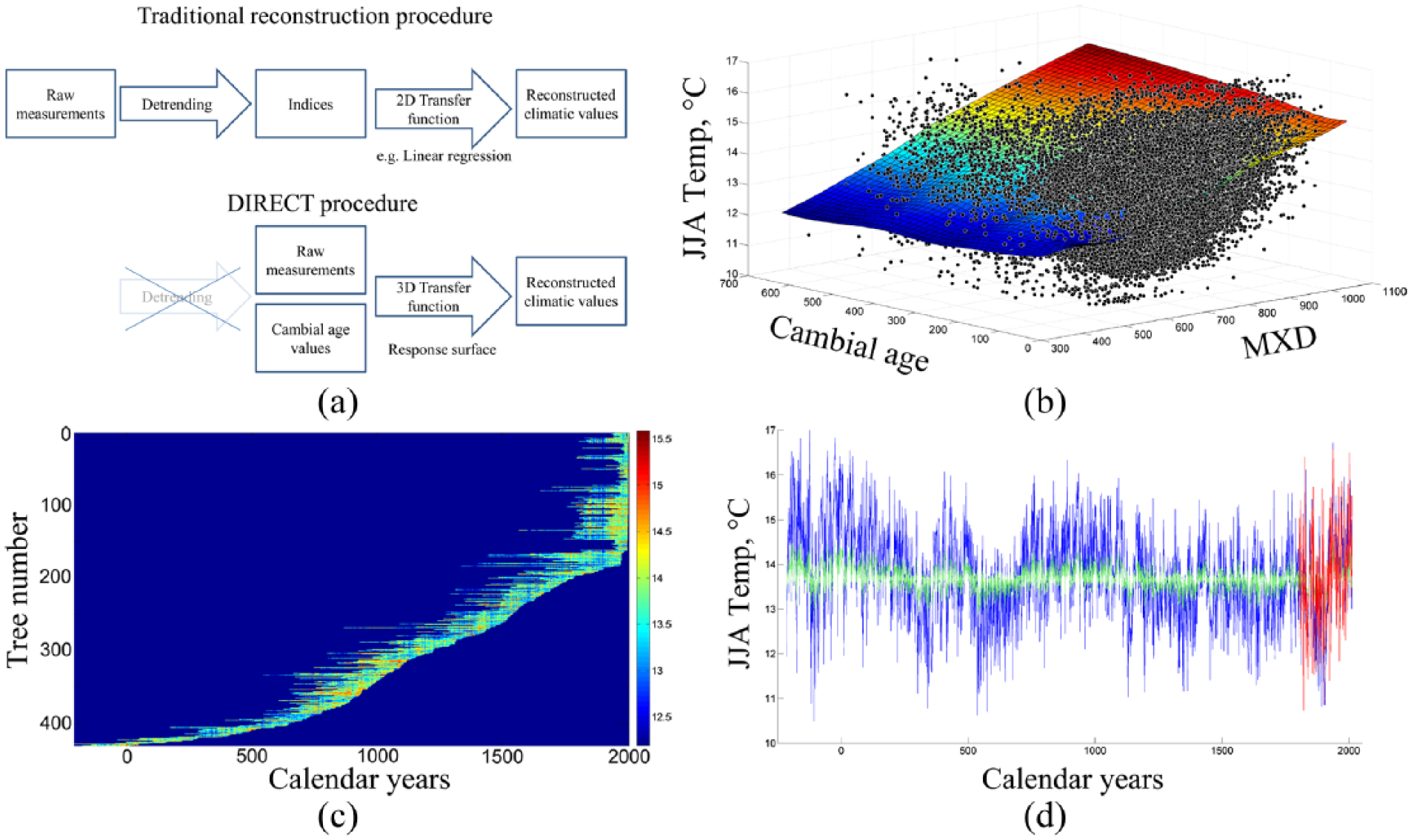
The DIRECT algorithm applied for the MXD of northern Fennoscandia: (a) The concept of the DIRECT compared with the traditional reconstruction procedure from tree-ring data; (b) The 3D surface is constructed as a transfer function model. The cloud of tree-ring data (black dots) over the instrumental period (AD 1802–2010) defined by MXD (x-axis), cambial age (y-axis) and JJA temperature (z-axis) for each tree ring smoothed by the 3D surface (coloured); (c) The transfer function, which was previously obtained as the 3D surface, is employed to transform each individual tree ring (with its MXD value and cambial age) into a temperature estimate (shown in colour). Tree rings are presented in series that correspond to individual trees; and (d) Averaging the individual values of temperature estimates for each calendar year and rescaling the variance of the mean reconstruction. The mean temperature reconstruction estimate time-series (green line) and the final rescaled reconstruction (blue line) are compared with the instrumental climate record (red).

Note that employing the cambial age as one of the explanatory variables simplifies how the tree-ring data can be transformed into estimates of climate variability. First, the use of mean chronology is unnecessary as the growth values are included in the calibration model as separate units; each value represents the tree-ring growth for a particular tree, age and year. A large number of growth values are available for modelling the 3D surface compared with the traditional approach, in which the number of annual growth values may be equivalent to the yearly length of the calibration period. Second, the detrending of tree-ring series to remove their non-climatic variations is unnecessary. Instead, the age-dependence in tree growth is simultaneously solved with the climate-dependence in the growth.

First step – Constructing the 3D surface

The first step of the DIRECT is to construct a surface that serves as a 3D representation of the age-dependent growth response to climate variability (Figure 1b). The exploited dimensions of cambial age, tree-ring value (MXD) and climatic parameter (JJA temperature) are employed to locate each tree ring into 3D space. The cloud of the tree-ring data, in which each point represents a ring formed during the instrumental period (i.e. the period with available climatic information), is smoothed by the thin-plate smoothing spline (Duchon, 1977) to construct the 3D surface. In this study, the smoothing was performed using MATLAB^® Curve Fitting Toolbox and the tpaps function. The rigidity of the surface is regulated by the smoothing parameter p, which represents a number between 0 and 1. As the smoothing parameter varies from 0 to 1, the smoothing spline varies from the least-squares approximation to the data by a linear polynomial when p is 0 to the thin-plate spline interpolant to the data when p is 1. To select an appropriate value of the parameter while avoiding overfitting (e.g. Figure S1c, available online), a cross-validation approach for constructing a surface on a randomly selected 50% of the sample was performed, and the selected parameter was evaluated using the data withheld from the surface construction. The smoothing value qualified as a robust value for the MXD data: 8 × 10⁻⁷.

Second step – Reconstructing climate for individual tree rings

After determining the 3D surface as a transfer function model, the next step of the DIRECT method proceeds via transformation of the individual tree rings into climate estimates (Figure 1c). Each individual tree ring represented by its MXD value and cambial age is utilized to derive a temperature estimate for corresponding calendar year. During this step, MXD and cambial age values are virtually equivalent in their effect on reconstructed temperature; thus, no special procedure (detrending) is required to separately eliminate the effect of age.

Third step – Averaging by year

As the next step of the DIRECT, the reconstructed climate estimates for each calendar year are averaged into a single time-series (Figure 1d).

Fourth step – Rescaling

The fourth and final step is to rescale the annual variations of the obtained palaeoclimate reconstruction. Compared with the traditional dendroclimatic approach, the DIRECT averages the proxy series after they have been transformed into palaeoclimate estimates. Any lack of correlativity among these series is known to produce lessened and underestimated variance in the mean time-series (Osborn et al., 1997). In addition, the smoothing of the initial data by a 3D surface (Step 1) causes a loss of its original variance. Therefore, the obtained mean climate estimate time-series is rescaled to exhibit the mean and variance that are equivalent to the instrumental temperatures (Figure 1d). These results were achieved using both the variance adjustment and the smoothed series variance adjustment approaches (Lee et al., 2007). The former is applied to the unsmoothed data, whereas the latter is applied subsequently to the data smoothed using the 15-year moving average (Matskovsky and Helama, 2014). Next, the mean and the variance were estimated for both the mean reconstruction and the instrumental temperature record over the calibration period. Finally, the mean reconstruction was scaled to represent the mean and standard deviation of the instrumental temperature record using the parameters estimated from the smoothed time-series.

Estimating uncertainties

Uncertainties of the temperature reconstruction were expected to originate from two independent sources. The first type of uncertainty is associated with the data replication, and the second type of uncertainty is associated with the instrumental period. The instrumental period is employed for 3D surface modelling, and the associated uncertainty about this surface affects the total period reconstruction. The estimation was performed using a bootstrapping procedure that is tailored to the DIRECT method. The sample of interest was resampled 1000 times with replacement. In the case of the first uncertainty type, the sample consisted of the reconstructed temperature values, which were derived from individual tree rings for each calendar year. In the case of the second uncertainty type, the sample comprised all years in the instrumental period, the corresponding temperatures and the tree rings formed during these years. Note that the second uncertainty can only be estimated for the pre-instrumental period as the instrumental period is bootstrapped for the calculations. Consequently, the bootstrap distributions of the statistics were obtained. First, we utilized α/2 × 100 and (1 − α/2) × 100 percentiles of this distribution to estimate the confidence limits, with α = 0.05. To estimate the uncertainty coming from both sources, α = (0.05)^0.5 was employed to compute the final 95% confidence interval. These calculations assumed that the uncertainties of the two types are independent.

Calibration and verification statistics

The instrumental period (AD 1802–2010) was divided into early (AD 1802–1906) and late (AD 1907–2010) periods to be employed as calibration and verification periods and vice versa to produce the summer (June through August) temperature reconstruction. In this manner, the evaluation of the reconstruction that was built using the DIRECT method follows common approaches and statistics to assess the quality of the tree-ring based palaeoclimate reconstruction. The statistics included the coefficient of determination (R²), the Pearson correlation coefficient (r), the reduction of error (RE), the coefficient of efficiency (CE) and the root mean square error (RMSE; Cook et al., 1994).

Estimation of long-term temperature trends

Previous studies have emphasized the interest in revealing the long-term temperature trends in tree-ring based temperature reconstructions (Esper et al., 2012, 2014; Helama et al., 2012; Mann et al., 1999). This trend line can be simply derived using linear regression; however, this estimation disregards the uncertainty in the underlying data. A bootstrap analysis that is tailored for estimating the trend in the tree-ring chronology of varying sample replications was performed by generating 1000 reconstructions using resampling with replacement. For each reconstruction, a number of randomly selected tree-ring series were replaced by another randomly selected series from the complete dataset. The trend line can be estimated 1000 times for each of the mean reconstructions using the limited number of series that were employed to calculate the mean, which enabled the estimation of uncertainty around the long-term trend. The estimates of temperature change were compared with the previously obtained estimations for dendroclimatic studies in the study region (Esper et al., 2012, 2014; Melvin et al., 2013).

Comparisons with RCS-based temperature reconstruction

The DIRECT-based temperature reconstruction was compared with the reconstruction produced using the traditional dendroclimatic approach, that is, RCS. The smoothing of the standardization curve was performed using time-varying response smoothing (Melvin et al., 2007) and a cubic spline with 50% variance cut-off (Cook and Peters, 1981), in which the spline stiffness for each year is equivalent to the cambial age in years added by 15 years. The mean MXD chronology was computed by averaging the processed MXD series into a mean chronology. The RCS-based palaeotemperature record was achieved using smoothed variance adjustment (Lee et al., 2007). First, the 15-year moving average was employed to smooth the tree-ring chronology and the temperature record. Second, the mean and the variance were estimated for both of the smoothed time-series over the calibration period. Third, the chronology was scaled to the climate record using the parameters estimated from the smoothed time-series.

Results

Age-dependent MXD response to temperature

Comparing the climate–growth associations in 3D space with cambial age and using the MXD value of individual rings enables the detection of instability in these relationships. Examination of the 3D surface (Figure 1b) transverse to the axis of cambial age illustrates how the age distinctly influences the temperature-dependent MXD production (Figure 2). This dendroclimatic relationship is positive but not linear. The rings younger than 150 years exhibit a notable non-linearity in their response to mean summer temperature; it appears that the MXD production is not noticeably enhanced in young trees until the observed temperature increases above 13°C. Beyond this temperature, a weaker response becomes evident.

Figure 2.

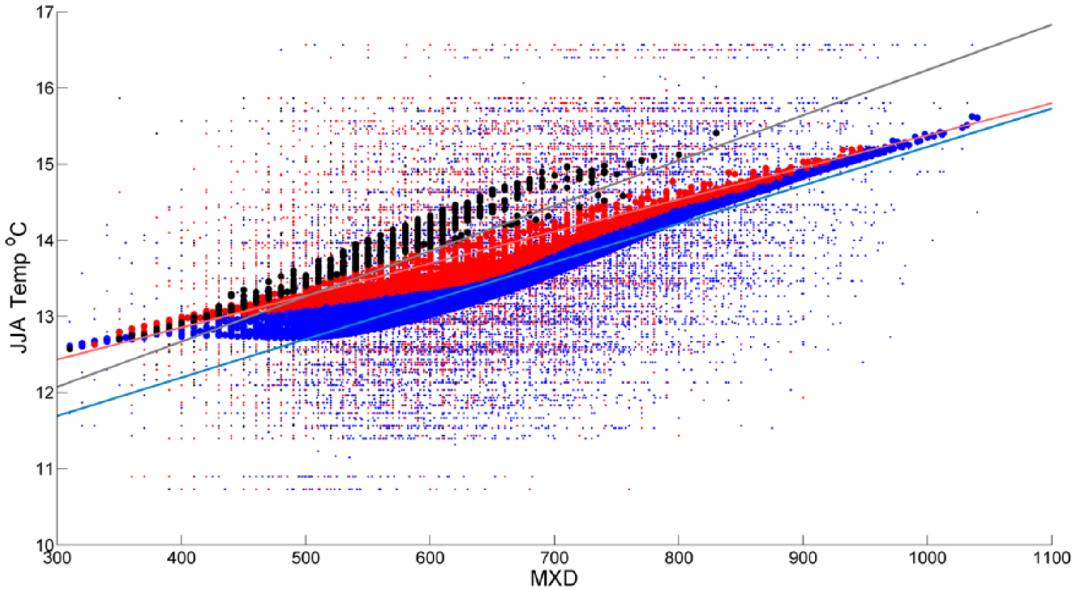
Illustrating the climate–MXD relations for three different age classes (blue dots for tree rings of 1–150 years, red dots for tree rings of 151–400 years, and black dots for tree rings older than 400 years). Smaller dots show the individual MXD values relative to instrumental JJA temperatures over the instrumental period (AD 1802–2010). Larger dots show different age parts of the 3D surface – the mean JJA temperatures for each (MXD, Cambial age) pair. Straight lines exemplify the total difference in the linear temperature–MXD relations for each of the three age classes (the lines generated using linear regression).

A similar feature is also observed for older pines. In the age class of 151- to 400-year-old trees, the temperature–MXD linkage is more gradual in conditions below 13.5°C compared with the growth response to temperatures above this level. Hence, the MXD production becomes more responsive to temperature variations above this boundary. However, the MXD may not provide equally reliable proxy for colder temperature variations. The generic slopes of the climate–growth relationships (as exemplified by straight lines in Figure 2) differentiate between the age classes. These results provide a more complex view of MXD production, its temperature-dependence, and its use as a temperature proxy than previously appreciated. DIRECT helps to overcome these circumstances as the use of the 3D surface considers any non-linearity that is inherent to climate–proxy relations.

Temperature reconstruction using the DIRECT

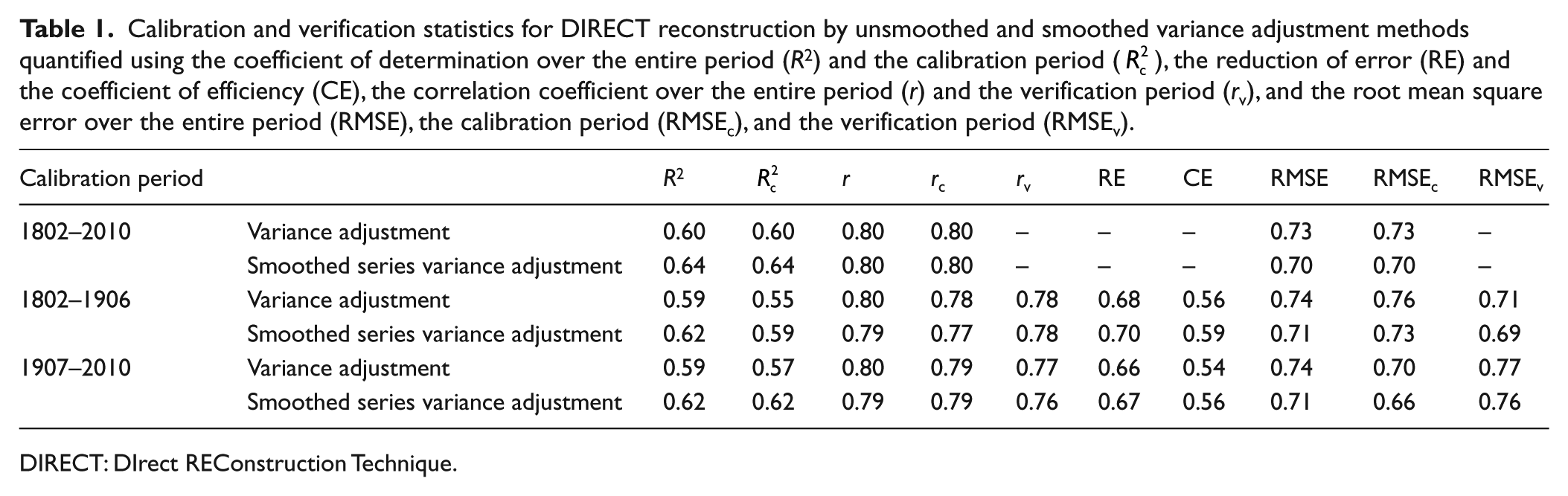
New DIRECT-based temperature reconstructions were derived using both variance adjustment and smoothed series variance adjustment approaches. These calibrations and verifications of the mean reconstruction (Table 1) using these approaches explain 55% to 62% of the instrumental temperature variance over the sub-periods (AD 1802–1906 and 1907–2010). The smoothed series variance adjustment produced larger coefficients of determination (R²) as determined over the same sub-periods. The reduction of error (RE) and coefficient of efficiency (CE) statistics showed significantly positive values, which indicate real skill in the reconstructions (refer to Cook et al., 1994). Note that the RMSEs for the smoothed series variance adjustments were invariably smaller compared with the variance adjustment approach in Step 4 of the algorithm.

Table 1.

Calibration and verification statistics for DIRECT reconstruction by unsmoothed and smoothed variance adjustment methods quantified using the coefficient of determination over the entire period (R²) and the calibration period ( $R_{c}^{2}$ ), the reduction of error (RE) and the coefficient of efficiency (CE), the correlation coefficient over the entire period (r) and the verification period (r_v), and the root mean square error over the entire period (RMSE), the calibration period (RMSE_c), and the verification period (RMSE_v).

Calibration period		R ²	$R_{c}^{2}$	r	r _c	r _v	RE	CE	RMSE	RMSE_c	RMSE_v
1802–2010	Variance adjustment	0.60	0.60	0.80	0.80	–	–	–	0.73	0.73	–
	Smoothed series variance adjustment	0.64	0.64	0.80	0.80	–	–	–	0.70	0.70	–
1802–1906	Variance adjustment	0.59	0.55	0.80	0.78	0.78	0.68	0.56	0.74	0.76	0.71
	Smoothed series variance adjustment	0.62	0.59	0.79	0.77	0.78	0.70	0.59	0.71	0.73	0.69
1907–2010	Variance adjustment	0.59	0.57	0.80	0.79	0.77	0.66	0.54	0.74	0.70	0.77
	Smoothed series variance adjustment	0.62	0.62	0.79	0.79	0.76	0.67	0.56	0.71	0.66	0.76

DIRECT: DIrect REConstruction Technique.

The same patterns of test statistics were observed for the total instrumental period (AD 1802–2010). Over this period, the mean reconstruction explained 60% of the instrumental temperature variance using the variance adjustment and 64% of the corresponding variance using the smoothed series variance adjustment approach. Additionally, the RMSEs for the latter approach were smaller than for the former approach. These statistics implied improved skill of the smoothed series variance adjustment in producing the final reconstruction. Consequently, this approach was applied in Step 4 of the DIRECT to produce the JJA temperature reconstruction for subsequent comparisons.

The new DIRECT reconstruction closely follows the observed temperature variability over the instrumental period (Figure 3a). The reconstruction shows a highly variable temperature history over the Common Era (Figure 3b). The main characteristics of the new reconstruction are represented in its low-frequency temperature variability. The modern warming is preceded by the multi-centennial period of cooler summer temperatures, often known as the ‘Little Ice Age’ (LIA; Bradley and Jones, 1993; Mann et al., 2009; Matthews and Briffa, 2005). In addition, the modern warming is matched with the period of similarly warm temperatures from the 8th century to the 11th century AD, which is analogous with the ‘Medieval Climate Anomaly’ (MCA; Goosse et al., 2012; Graham et al., 2011; Mann et al., 2009). The reconstruction also provides evidence of warm temperatures during the first BC/AD centuries. Similar features of the reconstruction were evident with experimental reconstructions, in which the modelling of the 3D surface was performed using differing smoothing parameters (Figures S1 and S2, available online), evolutionary intervals of calibration period (Figure S3, available online), and different numbers of trees (i.e. subsets of the complete dataset) in the reconstruction (Figure S4, available online).

Figure 3.

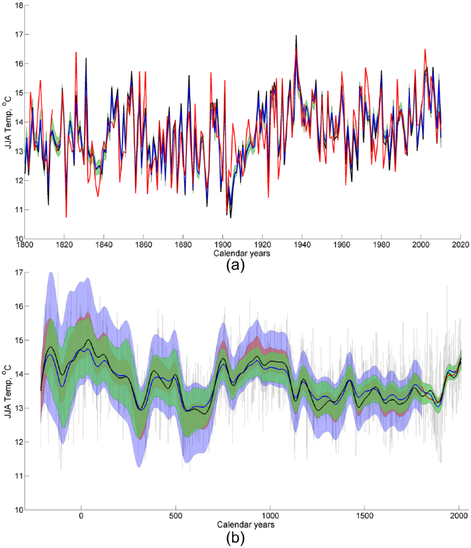
Instrumental JJA temperatures (red), the DIRECT- (blue) and RCS-based (black) reconstructions, and uncertainty of DIRECT reconstruction: data replication uncertainty (green shading), instrumental period uncertainty (red shading) and combined uncertainty (blue shading): (a) Instrumental period and (b) Reconstruction period. Series are smoothed by 100-year splines. Unsmoothed DIRECT reconstruction also shown in grey.

We note a number of significant differences when two alternative reconstructions were produced using only the high and low MXD values for respective DIRECT reconstructions (Figure 4). Compared with the DIRECT reconstructions, which were based on all available MXD values, the two artificially created reconstructions produce a final temperature reconstruction which is a combination of high and low MXD derivatives. In this regard, this comparison between the high-MXD reconstruction and the low-MXD reconstruction and their corresponding time-varying sample replications (Figure 4) demonstrates how the low-frequency variability is stored in the tree-ring data. The number of high value MXD rings increases during the MCA and the most recent era, whereas the number of low value MXD rings during the LIA is high. Although the quantity of the tree-ring proxy is important in the assessment of the mean proxy value, the number of high- and low-MXD rings contributes to the mean proxy value and its low-frequency variations.

Figure 4.

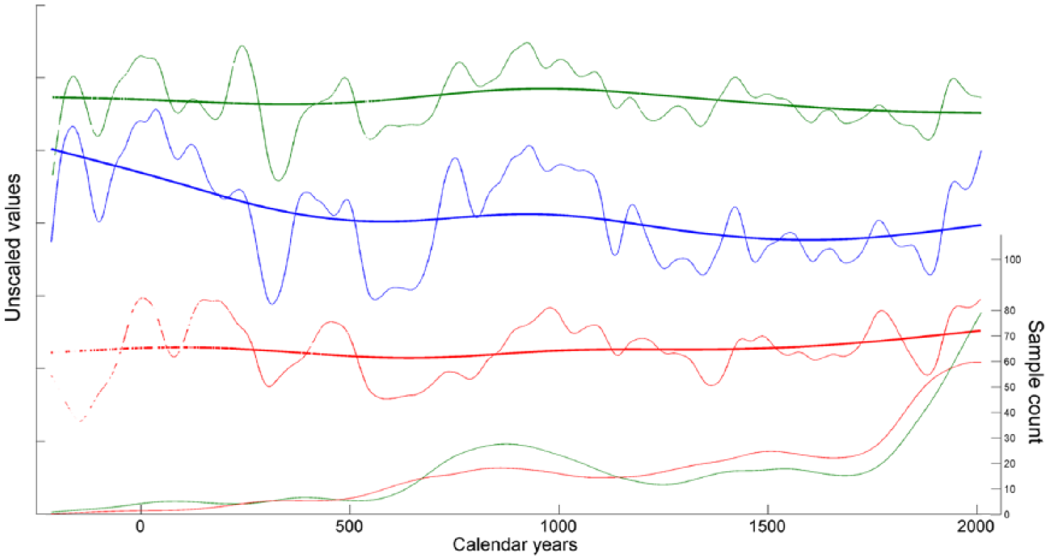
Comparison of DIRECT reconstructions based on high (green) and low (red) MXD values contrasted by the DIRECT reconstruction based on all available MXD values (blue). Replication of rings with high (green) and low (red) densities is shown. The fourth step (rescaling) of the DIRECT algorithm is omitted for visual comparison reasons. Annual time-series are smoothed with 100- and 300-year splines.

The new palaeoclimate evidence inferred from the DIRECT reconstruction is contrasted with the RCS-based reconstruction derived from the identical MXD data. This comparison is intended to highlight any differences between our new and conventional dendroclimatic temperature reconstructions.

Comparison of DIRECT- and RCS-based reconstructions

Our new DIRECT-based reconstruction is similar to the RCS-based reconstruction over the instrumental period (Figure 3). The Pearson correlation between the reconstructions over this period is 0.983. In addition to visual comparison, the two reconstructions can be compared by their correlations with the instrumental temperature record. Over the early period, the DIRECT (Table 1) and RCS reconstructions explained 59% and 58%, respectively, of the instrumental temperature variance, whereas over the late period the correlations were 62% and 60%, respectively. Over the entire instrumental period, the DIRECT- and RCS-based reconstructions explained 64% (refer to Table 1) and 62%, respectively, of the instrumental temperature variance. Although these percentages are similar, the values indicate a slight improvement in R² when the DIRECT method was employed.

The DIRECT and RCS reconstructions remain comparable over the first (AD 1–1000) and second (AD 1001–2000) millennia with inter-correlations of 0.986 for both periods. In both of the reconstructions, the coolest years occurred in AD 574 and the warmest years occurred in AD 1937 and 125 BC for the DIRECT reconstruction and RCS reconstruction, respectively. The maximum absolute difference between the reconstructions was 1.2°C (for AD 1453). Although these statistics are obtained for the annual variability in the reconstructed temperatures, the low-frequency comparison reveals a set of differences between the DIRECT reconstruction and RCS reconstruction. The warmest 30-year periods for the DIRECT reconstruction and RCS reconstruction were AD 23–52 and 21–50, respectively, over which the reconstructed temperatures remained 1.26°C warmer and 1.68°C warmer, respectively, than the mean temperatures over the AD 1901–2000 period in the corresponding reconstructions. The coolest 30-year periods for the DIRECT reconstruction and RCS reconstruction were AD 536–565 and 1452–1481, respectively, over which the temperatures in both cases remained 1.18°C cooler than the mean temperature of the 20th century. The difference between the warmest 30-year period and the coolest 30-year period translates into temperature amplitudes of 2.42 and 2.86°C, respectively, which reveals larger climate fluctuation in the RCS reconstruction.

A similar comparison was made using 100-year periods. While the DIRECT reconstruction exhibited the warmest centurial interval over the AD 25–124 period, the RCS reconstruction showed the warmest corresponding spell over the 31 BC–AD 70 period. For these intervals, the temperature departures indicated 0.87 and 1.12°C warmer climates compared with the AD 1901–2000 period in the DIRECT reconstruction and RCS reconstruction, respectively. The coolest 100-year periods occurred in AD 536–635 and 572–671, respectively, over which the temperatures of the DIRECT reconstruction and RCS reconstruction appeared 0.91°C cooler and 0.9°C cooler, respectively, than the 20th century. The corresponding temperature amplitudes of 1.79 and 2.02°C demonstrate a larger climate fluctuation in the RCS reconstruction. The maximum differences between the 100-year periods of the DIRECT reconstruction and RCS reconstruction are +0.24°C for AD 1206–1305, −0.28°C for 105–5 BC and AD 22–121.

Comparison of long-term temperature trends

Negative trend lines, that is, a stronger long-term temperature cooling, were observed for the RCS reconstruction for various intervals when the two reconstructions were compared over the past two millennia (Table S1, available online). These trends indicated a cooling of approximately 0.6°C (significant at α = 0.05) over the Common Era for DIRECT reconstruction (Figure S5, available online) and 0.8°C for RCS reconstruction. Over the past 1500 years, the indications of long-term cooling were stronger for RCS compared with the DIRECT reconstructions (Table S1, available online).

Interesting comparisons can also be made between the long-term temperature trends of the DIRECT reconstruction and other studies (Esper et al., 2012, 2014; Matskovsky and Helama, 2014; Melvin et al., 2013). The reconstructions based on tree-ring material from northernmost Swedish Lapland (Melvin et al., 2013) showed a significantly reduced long-term cooling. The long-term change in this proxy data is positive for the AD 517–2006 period, whereas the other reconstructions showed indications of cooling. Considering this feature of the Finnish/Swedish dataset, the strong cooling trends that were recently observed using the Finnish data (Esper et al., 2012, 2014) can be expected because of the origin of these data. The DIRECT reconstruction (which is a composite of both Finnish data and Swedish data) showed a bi-millennial trend of cooling comparable with the RCS-based reconstructions inferred from Finnish data (Esper et al., 2012, 2014). These analyses demonstrate the robustness of the DIRECT reconstruction for capturing the long-term climatic trend during the Common Era.

Discussion

The performance of the DIRECT and the RCS methods is similar when estimating the low-frequency temperature variability in the Common Era. The DIRECT method produces a number of features characteristic of low-frequency palaeoclimate information. We note that both reconstructions – the DIRECT and RCS – reproduced the main features of the temperature variations over the Common Era. One noticeably large difference between the DIRECT and RCS reconstructions is during the late-MCA, the 10th century AD and the 11th century AD, when the RCS reconstruction showed considerably warmer temperatures (Figure 3b). Interestingly, this interval coincided with the period in which the experimental reconstructions primarily diverged when these reconstructions were produced using artificially reduced sample replication (Figure S4, available online). Additionally, the RCS method is known to be prone to systematic biases near the beginning and end of the series (Briffa and Melvin, 2011). Conversely, the detrending end effect is not an issue with DIRECT reconstruction for which the growth trend/detrend issues are virtually absent. Note that the MXD dataset is relatively well-replicated over the majority of its length. If the replication had been smaller, a number of similar or more apparent biases could have been observed. We anticipate that these biases may reduce the quality of the present RCS reconstruction.

A major benefit of the 3D surface and the DIRECT method is that this methodology considers the difference in the climatic responses of trees of different ages and readily applies the obtained age-dependent relationships to derive the palaeoclimate estimates. Previously, the age-dependent growth responses have been demonstrated for Scots pine in Scandinavia (Linderholm and Linderholm, 2004) and several other tree species and regions (e.g. Carrer and Urbinati, 2004; Copenheaver et al., 2011; Wu et al., 2013). The 3D surface produced using our method provides a means for visualizing, quantifying and utilizing the reconstruction of the potentially differing climatic responses. This capability is derived from a construction of the 3D surface, which has a different shape and describes the climate–growth relationships for different biological ages. This feature analysis is not possible for reconstructions that are dependent on tree-ring indices as the indices of different biological ages are routinely mixed in averaging a mean chronology, which is then used to construct the transfer function. The use of a 3D surface, as applied in the DIRECT, provides a means for both visualizing and quantifying the potentially differing climatic response of trees of different ages.

Although our analyses have concentrated on palaeoclimate implications, the DIRECT may possess potentials for dendroecological studies. Given that the age-dependency in tree growth response appears unexplored but is a potentially arising dendroecological topic, the 3D surface can be employed to provide details about the growth response to climatic variations and the shape of this surface can be employed to quantify the possibility of age-dependency in this response.

Limitations of the DIRECT method

In addition to the benefits, a set of limitations may affect the performance of the DIRECT method. First, a considerably high amount of data for the instrumental period is needed to construct the 3D surface. A lack of data during the instrumental period will unavoidably increase the model uncertainty. A common feature of tree-ring chronologies is that the most recent end of the chronology and the instrumental period are predominantly covered by biologically old trees. Theoretically, if the instrumental period is shorter than the biological age of these trees, a part of the plain that is shaped by the cambial ages and growth values would lack the data that are required to bridge the gap over the part of the plain to be covered by cambially young rings. This requirement can be feasibly fulfilled by a proper sampling strategy, that is, by coring old trees and sampling a representative set of young trees. Second, DIRECT transforms the growth values into climate variability via a statistical model that is applied in 3D space and incorporates tree-ring measurements, cambial age and climate data. The model construction necessitates that the growth responses are profoundly linked to a single climatic factor. The MXD production of our northern pines appears to be largely controlled by the summer temperature variability. However, control of MXD by several climatic factors would impair the analyses and make the DIRECT reconstruction unfeasible. A third possible limitation of the methodology applied in this paper is that the limiting factor must be determinable using standard dendroclimatic methods (e.g. Biondi and Waikul, 2002) prior to the construction of the 3D surface and prior to its application for reconstruction purposes. The last two limitations are natural limitations of any reconstruction using a transfer function, but they get additional implications in DIRECT which unites standardization and transfer function. Fourth, the computational cost is large compared with commonly applied standardization methods. The highest incurred computational cost is related to the construction of the 3D surface to be smoothed by the thin-plate smoothing spline. These costs are multiplied by the use of cross-validation and/or bootstrapped uncertainty estimates, as applied in this study. Fifth, the use of a reduced set of tree rings that only cover the instrumental period, which represent the age-related MXD production, may be considered to be a limitation. This limitation means that it is assumed that the age-dependency of MXD production did not change during the reconstruction period.

New palaeoclimate evidence

The DIRECT reconstruction was shown to achieve several beneficial characteristics of low-frequency palaeoclimate information. We employ this advantage to obtain new palaeoclimate evidence inferred from the DIRECT reconstruction. Concomitantly, our interpretation concentrates on the low-frequency band of summer temperature variations that pertain to the period of June through August in the context of the most anomalous temperature events. The new reconstruction reproduces the variable temperature conditions during the past millennium, which represent a corresponding picture of temperature history over the Northern Hemisphere (Bradley and Jones, 1993; Goosse et al., 2012; Graham et al., 2011; Mann et al., 2009; Matthews and Briffa, 2005). The DIRECT reconstruction reveals long-term cooling during the LIA and considerable warming during the MCA. The 20th century marks a period of generally warm temperatures; however, the temperatures of the MCA were reconstructed to be warmer and the long duration of the former makes the MCA incomparable to the 20th-century warmth (Matskovsky and Helama, 2014).

On a century scale, the climatic cooling during the LIA was not as severe as the cooling phase during the 6th and 7th centuries AD as the ultimately coolest centennial period occurred in AD 536–635. The year AD 536 is known for its catastrophic and anomalous climate conditions, which prevailed over large areas of the Northern Hemisphere (Arjava, 2005; Baillie, 2008; Stothers, 1984, 1999). The summer of AD 536 was one of the coolest seasons as experienced in the study region in the context of the previous 7.6 thousand years (Helama et al., 2013; Jones et al., 2013). An analysis of multiple ice cores unveiled a signal that is consistent with the volcanic hypothesis for the event (Larsen et al., 2008). The climatic effects of volcanic eruptions are known, however, to persist over the first and second post-eruption years (Bradley, 1988; Robock, 2000). This extremely cool year was, however, followed by a century-scale cooling that represents one of the most eye-catching features of the reconstruction (Figure 3b). Parallel lines of evidence have recently identified an abrupt onset of the long-term LIA cooling as volcanically triggered regime shifts in climate (Gennaretti et al., 2014; Miller et al., 2012). These implications, which were derived from proxies of tree-ring and ice-cap growth from Arctic Canada and Iceland, were elaborated by previous millennium climate simulations, which suggest that short-lived volcanic eruptions may cause persistent regime shifts in the ocean circulation with spinning of the subpolar gyre and weakening of the Atlantic meridional overturning circulation (Schleussner and Feulner, 2013). Consequently, a significant cooling is expected to occur in the study region where the climate variability is coupled with natural instability of thermohaline circulation (Helama et al., 2009b). Cumulatively, the palaeoclimate evidence of the DIRECT may indicate the possibility of a volcano-induced onset of significantly reduced summer temperature over the northern Europe during the 6th and 7th centuries AD, which is similar to the previous findings about the climate system during the LIA.

A low-frequency feature that is common to several tree-ring proxy compilations is a millennia-long trend of temperature decline (Esper et al., 2012, 2014; Helama et al., 2012; Mann et al., 1999). This trend can be connected to the Milankovitch theory of orbital forcing, which is expected to cause decreased summer insolation in these regions over the present interglacial (Berger, 1978, 1988). Previously, the orbital forcing and consequent decline of summer insolation have been linked with macro- and megafossil evidence of retreating tree-limits in Fennoscandia through the Holocene (Eronen et al., 1999; Helama et al., 2004a; Kullman, 1992; Payette et al., 2002). The benefit of tree-ring data to trace this trend is that its slope can be determined for any range of calendar years. Although the DIRECT reconstruction corresponded with orbital forcing and previous MXD-based estimates (Esper et al., 2012) and exhibited trends of temperature cooling for various intervals over the past 1500–2000 years, the discrepancy among the DIRECT/RCS proxies of this study (Table S1, available online) and previous (Esper et al., 2012, 2014) studies and the Swedish RCS chronologies (Melvin et al., 2013) was inevitable. Why does the Swedish RCS chronology exhibit a positive trend over the past 1500 years? Does the negative long-term trend that originates from the Finnish MXD data represent an unbiased climatic signal?

Research previously suggested (Esper et al., 2012) that the enhanced sample replication was a reason to unveil the cooling trend in their RCS chronology. Our bootstrapping analysis did not, however, support this idea as the artificial reduction of replication did not produce positive trends in the case of DIRECT reconstruction (Figure S5, available online). Previous studies have indicated (Esper et al., 2014) a total positive and non-climatic long-term trend in the MXD chronology due to the natural decaying process of subfossil wood as the older discs are perceived lighter than younger discs. In contrast to this hypothesis, we argue that this lightening is likely to result from the dissolution of non-structural and secondary constituents of wood (Hillis, 1971, 1985) into the water and that the actual subfossil material of initially denser wood may preserve longer than subfossil wood of lesser density and durability. Consequently, a negative long-term trend in the wood density can be traced from a density analysis of extant samples due to taphonomical processes. We previously compared the metadata of Swedish (Melvin et al., 2013) and Finnish (Esper et al., 2012) MXD materials to conclude that one of the main differences between these sample arrays relates to their biogeographical aspects (Matskovsky and Helama, 2014). The Finnish material includes several boreal forest sites in the south and central Lapland, whereas the Swedish material is restricted to a much more northern timberline location. Whether the biogeographical matters contribute to the millennia-long trends in the chronologies and their respective reconstructions and whether the boreal forest MXD data behaves differently compared with timberline MXD data over corresponding timescales remain an unspecified issue.

Conclusion

The main purpose of this study was to introduce a new method for tree-ring-based reconstructions of past climate variability. One of the benefits of this DIRECT method is its avoidance of detrending and associated potential biases in performing dendroclimatic analyses. A tree-ring chronology can be purely expressed as climate (instead of growth) variability as the effects of cambial age are simultaneously considered when the data of individual tree-ring values are transformed into climate variability. An additional advantage of the methodology is that the modelled 3D surface visualizes and quantifies the age-dependent relationships between climate and growth. Compared with traditional dendroclimatic methods, in which the standardized series of tree-ring indices are averaged into a mean chronology, the 3D surface transforms the growth values into climate estimates by considering not only the cambial trends but also any potential variation in dendroclimatic associations as a function of tree age. Furthermore, the 3D surface has no linearity constraints.

Footnotes

Acknowledgements

We are grateful to the two anonymous reviewers for their valuable comments that helped to improve the manuscript. We acknowledge GHF Young for the text editing.

Funding

This study was funded by the Russian Science Foundation (grant no. 14-17-00645). Funding support to S Helama was provided by the Academy of Finland (grant no. 251441). V Matskovsky was partly supported by the Russian Foundation for Basic Research (grant no. 12-05-31126).

References

Arjava

(2005) The Mystery Cloud of 536 CE in the Mediterranean sources. Dumbarton Oaks Papers 59: 73–94.

Baillie

MGL

(2008) Proposed re-dating of the European ice core chronology by seven years prior to the 7th century AD. Geophysical Research Letters 35: L15813. DOI: 10.1029/2008GL034755.

Berger

(1978) Long-term variations of caloric insolation resulting from the earth’s orbital elements. Quaternary Research 9: 139–167.

Berger

(1988) Milankovitch theory and climate. Reviews of Geophysics 26: 624–657.

Biondi

Waikul

(2004) DENDROCLIM2002: A C++ program for statistical calibration of climate signals in tree-ring chronologies. Computers & Geosciences 30: 303–311.

Bradley

(1988) The explosive volcanic eruption signal in Northern Hemisphere continental temperature records. Climatic Change 12: 221–243.

Bradley

Jones

(1993) ‘Little Ice Age’ summer temperature variations: Their nature and relevance to recent global warming trends. The Holocene 3: 367–376.

Briffa

Melvin

(2011) A closer look at Regional Curve Standardization of tree-ring records: Justification of the need, a warning of some pitfalls, and suggested improvements of its application. In: Hughes

Diaz

Swetnam

(eds) Dendroclimatology: Progress and Prospects. Berlin: Springer-Verlag, pp. 113–145.

Briffa

Jones

Bartholin

. (1992) Fennoscandian summers from AD 500: Temperature changes on short and long timescales. Climate Dynamics 7: 111–119.

10.

Briffa

Jones

Schweingruber

. (1996) Tree-ring variables as proxy-climate indicators: Problems with low frequency signals. In: Jones

Bradley

Jouzel

(eds) Climatic Variations and Forcing Mechanisms of the Last 2000 Years. Berlin: Springer-Verlag, pp. 9–41.

11.

Briffa

Osborn

Schweingruber

. (2001) Low-frequency temperature variations from a northern tree ring density network. Journal of Geophysical Research 106: 2929–2941.

12.

Briffa

Osborn

Schweingruber

. (2002) Tree-ring width and density data around the Northern Hemisphere: Part 1, local and regional climate signals. The Holocene 12: 737–757.

13.

Carrer

Urbinati

(2004) Age-dependent tree-ring growth responses to climate in Larix decidua and Pinus cembra. Ecology 85(3): 730–740.

14.

Cook

(1990) Conceptual linear aggregate model for tree rings. In: Cook

Kairiukstis

(eds) Methods of Dendrochronology: Applications in the Environmental Science. Dordrecht: Kluwer Academic Publishers, pp. 98–104.

15.

Cook

Peters

(1981) The smoothing spline: A new approach to standardizing forest interior tree-ring width series for dendroclimatic studies. Tree-Ring Bulletin 41: 45–53.

16.

Cook

Briffa

Jones

(1994) Spatial regression methods in dendroclimatology – A review and comparison of two techniques. International Journal of Climatology 14: 379–402.

17.

Cook

Briffa

Meko

. (1995) The segment length curse in long tree-ring chronology development for paleoclimatic studies. The Holocene 5: 229–237.

18.

Cook

Briffa

Shiyatov

. (1990a) Tree-ring standardization and growth-trend estimation. In: Cook

Kairiukstis

(eds) Methods of Dendrochronology: Applications in the Environmental Science. Dordrecht: Kluwer Academic Publishers, pp. 104–123.

19.

Cook

Shiyatov

Mazepa

(1990b) Estimation of the mean chronology. In: Cook

Kairiukstis

(eds) Methods of Dendrochronology: Applications in the Environmental Science. Dordrecht: Kluwer Academic Publishers, pp. 123–132.

20.

Copenheaver

Crawford

Todd

(2011) Fearer Age-specific responses to climate identified in the growth of Quercus alba. Trees 25(4): 647–653.

21.

D’Arrigo

Wilson

Jacoby

(2006) On the long-term context for late twentieth century warming. Journal of Geophysical Research 111: D03103. DOI: 10.1029/2005JD006352.

22.

Duchon

(1977) Splines minimizing rotation invariant semi-norms in Sobolev spaces. In: Schempp

Zeller

(eds) Lecture Notes in Math, vol. 571. Berlin: Springer-Verlag, pp. 85–100.

23.

Edwards

TWD

Graf

Trimborn

. (2000) δ¹³C response surface resolves humidity and temperature signals in trees. Geochimica et Cosmochimica Acta 64: 161–167.

24.

Eronen

Hyvarinen

Zetterberg

(1999) Holocene humidity changes in northern Finnish Lapland inferred from lake sediments and submerged Scots pines dated by tree rings. The Holocene 9: 569–580.

25.

Esper

Cook

Schweingruber

(2002) Low-frequency signals in long tree-ring chronologies for reconstructing past temperature variability. Science 295: 2250–2253.

26.

Esper

Cook

Krusic

. (2003) Tests of the RCS method for preserving low-frequency variability in long tree-ring chronologies. Tree-Ring Research 59: 81–98.

27.

Esper

Dutorn

Krusic

. (2014) Northern European summer temperature variations over the Common Era from integrated tree-ring density records. Journal of Quaternary Science 29: 487–494.

28.

Esper

Frank

Timonen

. (2012) Orbital forcing of tree-ring data. Nature Climate Change 2: 862–866.

29.

Fritts

(1976) Tree Rings and Climate. London: Academic Press.

30.

Fritts

Mosimann

Bottorff

(1969) A revised computer program for standardizing tree-ring series. Tree-Ring Bulletin 29: 15–20.

31.

Gennaretti

Arseneault

Nicault

. (2014) Volcano-induced regime shifts in millennial tree-ring chronologies from northeastern North America. Proceedings of the National Academy of Science of the United States of America 111: 10077–10082.

32.

Goosse

Crespin

Dubinkina

. (2012) The role of forcing and internal dynamics in explaining the ‘Medieval Climate Anomaly’. Climate Dynamics 39: 2847–2866.

33.

Graham

Amman

Fleitmann

. (2011) Support for global climate reorganization during the ‘Medieval Climate Anomaly’. Climate Dynamics 37: 1217–1245.

34.

Graumlich

(1991) Subalpine tree growth, climate, and increasing CO_2: An assessment of recent growth trends. Ecology 72: 1–11.

35.

Graumlich

(1993) A 1000-year record of temperature and precipitation in the Sierra Nevada. Quaternary Research 39: 249–255.

36.

Graumlich

Brubaker

(1986) Reconstruction of annual temperature (1590–1979) for Longmire, Washington, derived from tree rings. Quaternary Research 25: 223–234.

37.

Grudd

(2008) Torneträsk tree-ring width and density AD 500–2004: A test of climatic sensitivity and a new 1500-year reconstruction of north Fennoscandian summers. Climate Dynamics 31: 843–857.

38.

Helama

Holopainen

Macias-Fauria

. (2013) A chronology of climatic downturns through the mid- and late-Holocene: Tracing the distant effects of explosive eruptions from palaeoclimatic and historical evidence in northern Europe. Polar Research 32: 15866. DOI: 10.3402/polar.v32i0.15866.

39.

Helama

Lindholm

Timonen

. (2004a) Dendrochronologically dated changes in the limit of pine in northernmost Finland during the past 7.5 millennia. Boreas 33: 250–259.

40.

Helama

Lindholm

Timonen

. (2004b) Detection of climate signal in dendrochronological data analysis: A comparison of tree-ring standardization methods. Theoretical and Applied Climatology 79: 239–254.

41.

Helama

Makarenko

Karimova

. (2009a) Dendroclimatic transfer functions revisited: Little Ice Age and Medieval Warm Period summer temperatures reconstructed using artificial neural networks and linear algorithms. Annales Geophysicae 27: 1097–1111.

42.

Helama

Seppä

Bjune

. (2012) Fusing pollen-stratigraphic and dendroclimatic proxy data to reconstruct summer temperature variability during the past 7.5 ka in subarctic Fennoscandia. Journal of Paleolimnology 48: 272–286.

43.

Helama

Timonen

Holopainen

. (2009b) Summer temperature variations in Lapland during the Medieval Warm Period and the Little Ice Age relative to natural instability of thermohaline circulation on multi-decadal and multi-centennial scales. Journal of Quaternary Science 24: 450–456.

44.

Helama

Vartiainen

Kolström

. (2008) X-ray microdensitometry applied to subfossil tree-rings: Growth characteristics of ancient pines from the southern boreal forest zone in Finland at intra-annual to centennial time-scales. Vegetation History and Archaeobotany 17: 675–686.

45.

Hillis

(1971) Distribution, properties and formation of some wood extractives. Wood Science and Technology 5: 272–289.

46.

Hillis

(1985) Occurrence of extractives in wood tissues. In: Higuchi

(ed.) Biosynthesis and Biodegradation of Wood Components. Orlando, FL: Academic Press, pp. 209–228.

47.

Jones

Briffa

Barnett

. (1998) High-resolution palaeoclimatic records for the last millennium: Interpretation, integration and comparison with General Circulation Model control-run temperatures. The Holocene 8: 455–471.

48.

Jones

Briffa

Osborn

. (2009) High-resolution palaeoclimatology of the last millennium: A review of current status and future prospects. The Holocene 19: 3–49.

49.

Jones

Melvin

Harpham

. (2013) Cool North European summers and possible links to explosive volcanic eruptions. Journal of Geophysical Research 118: 6259–6265.

50.

Kaufman

(2014) A community-driven framework for climate reconstructions. Eos, Transactions of the American Geophysical Union 95: 361–362.

51.

Klingbjer

Moberg

(2003) A composite monthly temperature record from Tornedalen in northern Sweden, 1802–2002. International Journal of Climatology 23: 1465–1494.

52.

Kullman

(1992) Orbital forcing and tree-limit history: Hypothesis and preliminary interpretation of evidence from Swedish Lappland. The Holocene 2: 131–137.

53.

LaMarche

Jr (1982) Sampling strategies. In: Hughes

Kelly

Pilcher

(eds) Climate from Tree Rings. Cambridge: Cambridge University Press, pp. 2–6.

54.

Larsen

Vinther

Briffa

. (2008) New ice core evidence for a volcanic cause of the A.D. 536 dust veil. Geophysical Research Letters 35: L04708. DOI: 10.1029/2007GL032450.

55.

Lee

TCK

Zwiers

Tsao

(2007) Evaluation of proxy based millennial reconstruction methods. Climate Dynamics 31: 263–281.

56.

Linderholm

(2004) Age-dependent climate sensitivity of Pinus sylvestris L. in the central Scandinavian Mountains. Boreal Environment Research 9: 307–317.

57.

Linderholm

Gunnarson

Liu

(2010) Comparing Scots pine tree-ring proxies and detrending methods among sites in Jämtland, west-central Scandinavia. Dendrochronologia 28: 239–249.

58.

Ljungqvist

Krusic

Brattström

. (2012) Northern Hemisphere temperature patterns in the last 12 centuries. Climate of the Past 8: 227–249.

59.

Mann

Bradley

Hughes

(1999) Northern Hemisphere temperatures during the past millennium: Inferences, uncertainties, and limitation. Geophysical Research Letters 26: 759–762.

60.

Mann

Zhang

Rutherford

. (2009) Global signatures and dynamical origins of the Little Ice Age and Medieval Climate Anomaly. Science 326: 1256–1260.

61.

Matskovsky

(2011) Estimation of biases in RCS chronologies of tree rings. Journal of Siberian Federal University: Biology 4: 389–404 (In Russian).

62.

Matskovsky

Helama

(2014) Testing long-term summer temperature reconstruction based on maximum density chronologies obtained by reanalysis of tree-ring data sets from northernmost Sweden and Finland. Climate of the Past 10: 1473−1487. DOI: 10.5194/cp-10-1-2014.

63.

Matthews

Briffa

(2005) The ‘Little Ice Age’: Re-evaluation of an evolving concept. Geografiska Annaler 87A: 17–36.

64.

Melvin

(2004) Historical growth rates and changing climatic sensitivity of boreal conifers. Thesis, University of East Anglia, Available at: http://www.cru.uea.ac.uk/cru/pubs/thesis/2004-melvin/.

65.

Melvin

Briffa

(2014) CRUST: Software for the implementation of Regional Chronology Standardisation: Part 1. Signal-Free RCS. Dendrochronologia 32: 7–20.

66.

Melvin

Briffa

Nicolussi

. (2007) Time-varying response smoothing. Dendrochronologia 25: 65–69.

67.

Melvin

Grudd

Briffa

(2013) Potential bias in ‘updating’ tree-ring chronologies using Regional Curve Standardisation: Re-processing 1500-years of Torneträsk density and ring-width data. The Holocene 23: 364–373.

68.

Miller

Geirsdóttir

Zhong

. (2012) Abrupt onset of the Little Ice Age triggered by volcanism and sustained by sea-ice/ocean feedbacks. Geophysical Research Letters 39: L02708. DOI: 10.1029/2011GL050168.

69.

Osborn

Briffa

(2006) The spatial extent of 20th-century warmth in the context of the past 1200 years. Science 313: 841–844.

70.

Osborn

Briffa

Jones

(1997) Adjusting variance for sample-size in tree-ring chronologies and other regional mean timeseries. Dendrochronologia 15: 89–99.

71.

Payette

Eronen

Jasinski

JJP

(2002) The Circumboreal Tundra–Taiga Interface: Late Pleistocene and Holocene changes. Ambio Special Report 12: 15–22.

72.

Robock

(2000) Volcanic eruptions and climate. Reviews of Geophysics 38: 191–219.

73.

Salminen

(2009) The effect of temperature on height growth of Scots pine in northern Finland. Dissertationes Forestales 96: 1–39.

74.

Schleussner

Feulner

(2013) A volcanically triggered regime shift in the subpolar North Atlantic Ocean as a possible origin of the Little Ice Age. Climate of the Past 9: 1321–1330.

75.

Schweingruber

Bartholin

Schär

. (1988) Radiodensitometric-dendroclimatological conifer chronologies from Lapland (Scandinavia) and the Alps (Switzerland). Boreas 17: 559–566.

76.

Schweingruber

Kairiukstis

Shiyatov

(1990) Sample selection. In: Cook

Kairiukstis

(eds) Methods of Dendrochronology: Applications in the Environmental Science. Dordrecht: Kluwer Academic Publishers, pp. 23–35.

77.

Stothers

(1984) Mystery Cloud of A.D 536. Nature 307: 344–345.

78.

Stothers

(1999) Volcanic dry fogs, climate cooling, and plague pandemics in Europe and the Middle East. Climatic Change 42: 713–723.

79.

Warren

(1980) On removing the growth trend from dendrochronological data. Tree-Ring Bulletin 40: 35–44.

80.

Woodhouse

(1999) Artificial neural networks and dendroclimatic reconstructions: An example from the Front Range Colorado, USA. The Holocene 9: 521–529.

81.

Chen

. (2013) Age-dependent tree-ring growth responses of Schrenk spruce (Picea schrenkiana) to climate – A case study in the Tianshan Mountain, China. Dendrochronologia 31(4): 318–326.

Supplementary Material

Please find the following supplemental material available below.

For Open Access articles published under a Creative Commons License, all supplemental material carries the same license as the article it is associated with.

For non-Open Access articles published, all supplemental material carries a non-exclusive license, and permission requests for re-use of supplemental material or any part of supplemental material shall be sent directly to the copyright owner as specified in the copyright notice associated with the article.

0.00 MB