Calibrating aquatic microfossil proxies with regression-tree ensembles: Cross-validation with modern chironomid and diatom data

Abstract

We examine the ability of four different regression-tree ensemble techniques (bagging, random forest, rotation forest and boosted tree) in calibration of aquatic microfossil proxies. The methods are tested with six chironomid and diatom datasets, using a variety of cross-validation schemes. We find random forest, rotation forest and the boosted tree to have a similar performance, while bagging performs less well and in several cases has trouble producing continuous predictions. In comparison with commonly used parametric transfer-function approaches (PLS, WA, WA-PLS), we find that in some cases tree-ensemble methods outperform the best-performing transfer-function technique, especially with large datasets characterized by complex taxon responses and abundant noise. However, parametric transfer functions remain competitive with datasets characterized by low number of samples or linear taxon responses. We present an implementation of the rotation forest algorithm in R.

Keywords

bagging boosted regression tree partial least squares random forest rotation forest weighted averaging

Introduction

Quantitative environmental reconstructions prepared from aquatic microfossils have a multitude of applications, including environmental monitoring, palaeoclimate research, and the study of sensitivity, resilience and human impact in ecosystems. Starting in the 1970s, numerous quantitative approaches have emerged to infer palaeoenvironmental parameters from microfossil assemblages (Juggins and Birks, 2012). Key techniques in palaeolimnological reconstructions have been regression-based multivariate transfer functions such as weighted averaging (WA; Birks et al., 1990b) or weighted averaging-partial least squares (WA-PLS; ter Braak and Juggins, 1993), based on parametric estimation of taxon responses (e.g. linear or unimodal) using modern calibration data. Past environmental values are then predicted based on the modelled responses for the taxa found in the fossil assemblages. Such parametric transfer functions have been complemented by methods based on assemblage matching (the modern-analogue technique (MAT)) and less frequently by other approaches such as ones based on Bayesian statistics or artificial neural networks (Juggins and Birks, 2012).

While parametric transfer functions remain a cornerstone of palaeoenvironmental reconstruction, in other fields of quantitative ecology, such as species-distribution modelling, parametric modelling tools (e.g. generalized linear modelling) have been noted as having considerable limitations in modelling species–climate relationships. Consequently, ecologists have increasingly turned to so-called machine-learning (ML) algorithms, which explore the data while making minimal assumptions about the species–environment relationships (Elith et al., 2006; Zimmermann et al., 2010). Among the emerging ML-based modelling techniques are methods based on creating ensembles of regression-tree models. In recent years, there has been growing interest in applying such regression-tree ensembles in fossil proxy calibration and palaeoenvironmental reconstruction (Goring et al., 2010; Juggins et al., 2015; Salonen et al., 2012, 2014; Simpson and Birks, 2012). There is clear potential in such transfer of methodology, as while the typical aim of palaeoenvironmental reconstruction (i.e. quantifying past environmental change) differs from that of species-distribution modelling (predicting range shifts under climatic change), the two applications are similar with respect to the statistical modelling as both are underpinned by models of taxon response over environmental gradients.

Based on the general properties of regression trees, several potential advantages have been identified for tree ensembles as proxy-calibration tools. These include (1) their ability to model complex (e.g. bimodal) taxon responses, (2) their ability to deal with calibration datasets showing a diverse combination of response shapes, (3) their ability to model interactions between predictors, (4) their inherent selectivity in only using taxa showing an important response along the reconstructed gradient and (5) their sensitivity to rare indicator taxa (Juggins et al., 2015; Salonen et al., 2014). While these expected strengths are acknowledged, the empirical evidence about the performance of tree-ensemble methods in calibrating microfossil proxies is only starting to emerge. A general challenge in this work is the difficulty of evaluating the reliability of any proxy calibration (Juggins and Birks, 2012). Commonly used cross-validation (CV) schemes (e.g. leave-one-out (LOO)) can be susceptible to showing inflated performance in the presence of spatial autocorrelation (Telford and Birks, 2009) or correlated, ecologically significant secondary gradients (Juggins, 2013a), while the sensitivity to such confounding factors may vary between methods (Juggins et al., 2015; Salonen et al., 2014; Telford and Birks, 2009), considerably complicating between-methods comparisons. Meanwhile, the assessment of predictions prepared for down-core (fossil) data is often challenging because of limited prior information on the past environmental conditions (but see Telford and Birks, 2011). Goring et al. (2010) applied a single tree-ensemble method, the random forest (Breiman, 2001), in split-sampling tests with modern pollen samples. They found random forest to outperform WA/WA-PLS in predicting summer growing degree days but not in predicting summer precipitation, while MAT performed best with both variables. However, Goring et al. (2010) note the challenges in assessing the relative performance between methods because of spatial autocorrelation. Salonen et al. (2014) tested another tree-ensemble method, the boosted regression tree (BRT; De’ath, 2007), in pollen–climate calibration with inconclusive results as BRTs failed to consistently outperform WA and MAT in robust h-block CV. Two studies have tested BRTs using k-fold CV with modern diatom datasets, and found BRTs to not improve on parametric methods including WA and maximum likelihood calibration of response curves (MLRC) (Juggins et al., 2015; Simpson and Birks, 2012). However, when predicting for simulated fossil datasets, Juggins et al. (2015) found BRTs to often outperform WA and MLRC, especially in situations where some taxa mainly respond to a non-reconstructed secondary variable and independent past shifts occur in that secondary variable. In summary, while increasing evidence exists about the usefulness of tree ensembles from other applications (Simpson and Birks, 2012), the evidence on their ability to improve on classical parametric methods in calibration of fossil proxies remains limited and inconclusive.

Here, we test the ability of several tree-ensemble approaches in the prediction of environmental parameter values based on aquatic microfossil assemblages. The performance of tree ensembles is compared against commonly used parametric transfer-function techniques. We use six datasets, representing two key palaeolimnological proxies (diatoms and chironomids), several environmental response variables and three different continents (Europe, North America and Africa). The predictive ability with each dataset is assessed by applying a variety of CV schemes, where the selection of the most suitable CV scheme depends on the spatial structure of the individual dataset.

Materials and methods

Datasets

We test the predictive ability of different calibration approaches using six datasets, each consisting of samples of modern diatom or chironomid assemblages obtained from aquatic environments (mostly surface sediment samples from lakes and ponds) and observations on the modern values of an environmental variable that is considered to be an important environmental driver of species-distribution patterns (see references in Table 1 for more information on proxy–environment relationships). Details and references for the used datasets are presented in Table 1. The datasets differ considerably in terms of number of samples (69–622), number of predictor variables, that is, the number of diatom or chironomid taxa (78–652), and complexity of taxon response. All variables are continuous: taxon abundance percentages for all predictors and measured environmental values for the response variables.

Table 1.

Details and references for the datasets used.

Code	Location	Predictor	Response	No. of samples	No. of predictors	Gradient span	Cross-validation type	References
Dia–pH_UK	United Kingdom	Diatoms	Water pH	167	277	4.3–7.3	10-fold (10 repeats)	Surface water acidification Programme (Birks et al., 1990a; Stevenson et al., 1991)
Dia–pH_EU	Europe	Diatoms	Water pH	622	652	0.3–8.4	10-fold (10 repeats)	European Diatom Database Initiative (http://craticula.ncl.ac.uk/Eddi/jsp/index.jsp)
Dia–logEC	Uganda	Diatoms	Water log electrical conductivity	69	265	1.8–4.2	10-fold (10 repeats)	Mills and Ryves (2012)
Chi–Tjul	North America	Chironomids	Mean July air temperature (°C)	434	78	2.0–16.3	10-fold (10 repeats), h-block	Fortin et al. (2015)
Chi–depth	Massachusetts	Chironomids	Water depth (m)	98	82	0.3–9.3	Leave-one-cluster-out	Engels and Cwynar (2011)
Dia–colour	Finland	Diatoms	Water colour (mgPt/L)	225	214	5–350	Leave-one-cluster-out	Soininen et al. (2004) and Pajunen et al. (2016)

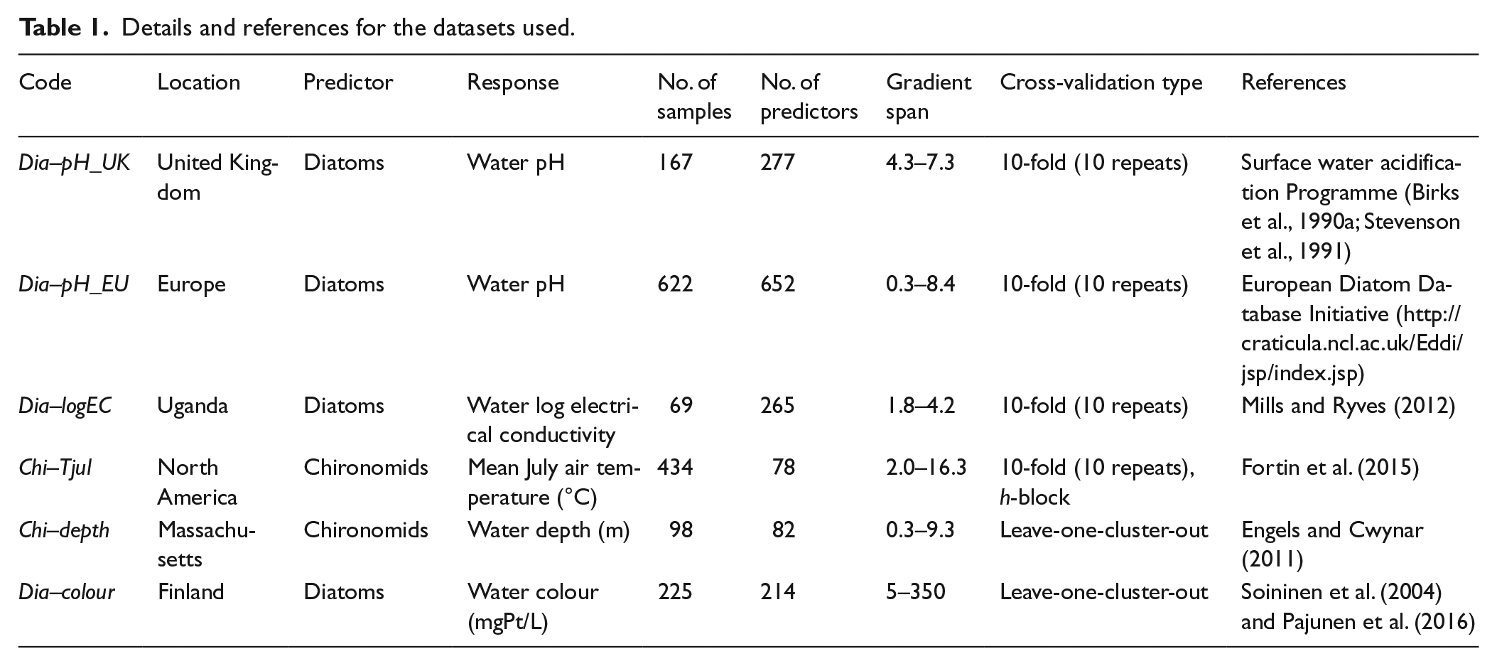
Two of these are lake diatom–water pH datasets, originating from the Surface Waters Acidification Programme of the United Kingdom (Dia–pH_UK) and the European Diatom Database Initiative (Dia–pH_EU). The latter dataset is considerably larger in terms of geographic span and number of samples. A third diatom dataset (Dia–logEC) is sampled from Ugandan crater lakes, with water log electrical conductivity (logEC) as the response variable. The fourth dataset (Chi–Tjul) consists of chironomid samples from North American lakes, with mean July air temperature (T_jul) as response variable. The final two datasets (Chi–depth, Dia–colour) share the key feature that they are spatially clustered, with each cluster alone sampling a significant portion of the environmental gradient. This allows a leave-one-cluster-out CV (LOCO CV; Wenger and Olden, 2012) to be performed with these datasets, in effect constituting a k-fold external CV and providing a robust estimate of predictive ability for new data. Chi–depth consists of chironomid assemblages sampled along depth gradients from seven lakes in southeast Massachusetts, with 5–25 samples from each lake and 98 samples in total (Figure 1a). We use water depth as the response variable with this dataset. Dia–colour consists of benthic diatom assemblages, sampled from stone surfaces in Finnish streams. We note that this is not a traditional palaeolimnological calibration dataset as the species samples come from stream epilithon and not lake surface sediment. While this dataset may not be directly applicable to palaeolimnological reconstructions, we use it here as the spatial structure of the data enables the LOCO CV to be performed, and the dataset can thus serve as a useful test case of the ability of different methods to model environment–diatom relations. The sampling locations form eight spatial clusters, with 13–59 sampling sites in each cluster and 225 samples in total (Figure 1b). We use water colour (mgPt/L) as the response variable with the Dia–colour dataset (e.g. Battarbee et al., 1997; Soininen et al., 2004; Steinberg, 2003). Water colour was chosen from a set of environmental factors identified in earlier work as important ecological drivers in this dataset, also including growing degree days, conductivity and total phosphorus (e.g. Pajunen et al., 2016; Soininen et al., 2004). With water colour, the individual clusters span overlapping segments of the gradient, a requirement for implementing the LOCO CV. Conductivity and growing degree days were rejected for not meeting this requirement, while total phosphorus was rejected for showing very poor performance in preliminary CV runs. Some samples from the high ends of the gradients were removed from Dia–colour (two samples with water colour >350 mgPt/L) and Chi–depth (six samples with water depth >9.3 m) as these gradient segments were only covered by a single sample cluster, making prediction of these values in LOCO CV impossible. Outliers identified by the dataset authors were removed from Dia–logEC (seven samples; for details, see Mills and Ryves, 2012) and Chi–Tjul (one sample; cf. Fortin et al., 2015).

Figure 1.

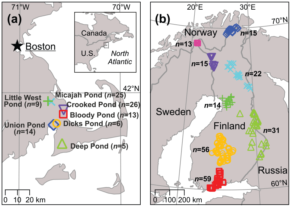
Maps of datasets (a) Chi–depth and (b) Dia–colour (see Table 1 for details). Different symbols indicate spatial cluster membership. Numbers of samples in each spatial cluster are indicated.

Calibration methods

We test four different algorithms for building regression-tree ensembles: bagging (Breiman, 1996), random forest (RaF; Breiman, 2001), rotation forest (RoF; Rodríguez et al., 2006) and BRT (De’ath, 2007). All four approaches build on the simple regression tree (De’ath and Fabricius, 2000), a commonly used and versatile data analysis tool. However, a weakness of the single-tree model is poor predictive ability for new data, a drawback of the simple model structure. The ensemble methods used here are based on improving the predictive ability by combining a large number of trees while still benefiting of many of the intrinsic advantages of a tree-based model (Simpson and Birks, 2012).

Bagging, RaF and RoF are closely related methods which all generate a set number of trees and calculate the prediction based on the mean of the predictions from the individual trees (or a majority vote for a categorical response). The three methods differ in that they use increasingly complex ways to introduce diversity into the ensemble. In bagging, each tree is built with a bootstrap sample of the training data. The bootstrap is also used in RaF, but additionally, only a random subset of the predictor set is provided when determining each tree split. In RoF, the individual trees are likewise built from bootstrap samples. However, in RoF, the training data predictor set for each tree is then divided into K random subsets, and principal component analysis (PCA) is applied separately on each subset. This creates a random rotation of the predictor space for each tree and adds a second layer of stochasticity into RoF model building. In effect, these introduced stochasticities force the individual learners (trees) to view the data in slightly different contexts (e.g. using a subset of samples or predictors) which helps the learners to produce diverse and complementary ‘rules of thumb’ which then enable the combined ensemble to predict accurately. In the ensemble building in bagging and RaF/RoF, new trees are calculated independently, without considering the predictive power of the previous trees. Our final tree-ensemble method, the BRT, differs significantly in that the ensemble is built sequentially, with each added tree aiming to explain the residuals of the previously fitted ensemble. The BRT can thus be likened to an additive regression model in which the individual terms are regression trees (e.g. Elith et al., 2008; Kuncheva and Rodríguez, 2007; Simpson and Birks, 2012). RaF and BRT have seen increasing use in palaeoecology (for a review, cf. Simpson and Birks, 2012; for more recent examples, cf. Felde et al., 2014; Juggins et al., 2015; Li et al., 2015; Salonen et al., 2012, 2014; Veloz et al., 2012; Zhao et al., 2012). Bagging or RoF has not, to our knowledge, been previously used in palaeoecology or palaeolimnology.

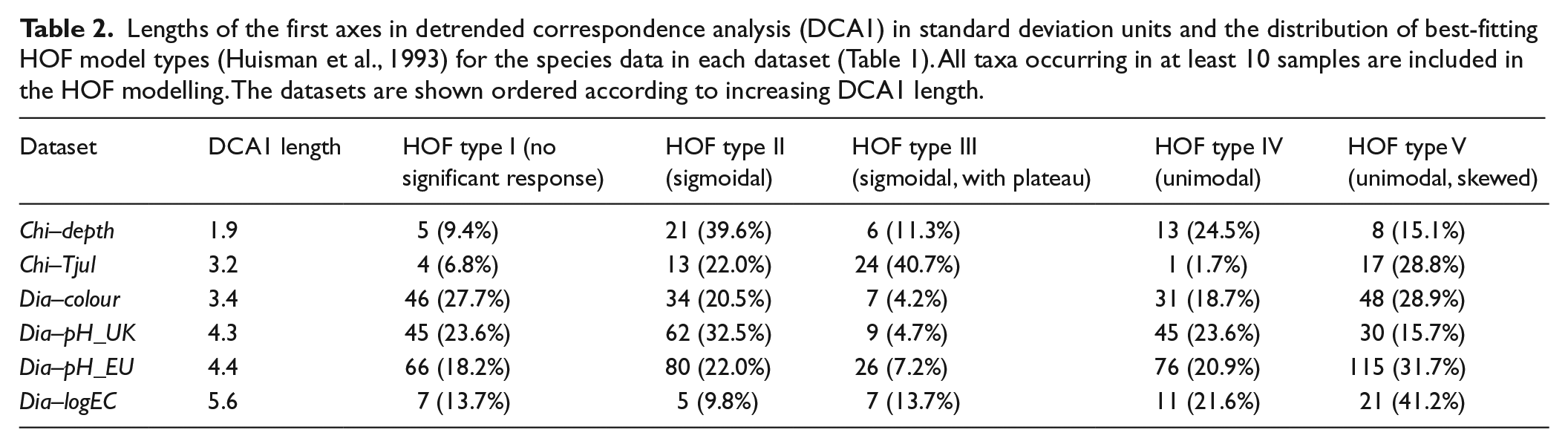
We also use three commonly used transfer functions to assess the performance of these tree-ensemble techniques against parametric methods: PLS, WA and WA-PLS. The three techniques differ in the shape of assumed response which is linear in PLS and unimodal in WA/WA-PLS (Juggins and Birks, 2012). To guide the choice between PLS and WA/WA-PLS, we fit HOF models to the percentage values of each taxon (Huisman et al., 1993; implemented using the R package eHOF (version 1.5.4; Jansen and Oksanen, 2013)). In HOF, increasingly complex parametric response models are fitted to determine the most complex model to give a statistically significant improvement in fit. In addition, we calculate for each dataset the lengths of first axes in detrended correspondence analysis (DCA), another commonly used method to choose between linear and unimodal modelling (Lepš and Šmilauer, 2003). The DCA first-axis lengths are shortest with the two chironomid datasets (Table 2). With these datasets, the predominant determined response, among taxa showing any significant response (i.e. the final fitted model type is other than I), is sigmoidal (Table 2; HOF model type II or III). A short DCA axis length (1.90) is found with Chi–depth, and we thus choose PLS with this dataset, as done in the original work of Engels et al. (2012). The authors of Chi–Tjul consider their dataset a borderline case between linear and unimodal modelling (Fortin et al., 2015), and here, we use both PLS and WA/WA-PLS with this dataset. With the remaining datasets, the DCA axis lengths are longer while the predominant response shape becomes unimodal (Table 1; model type IV or V), and thus, WA/WA-PLS is chosen with these datasets.

Table 2.

Lengths of the first axes in detrended correspondence analysis (DCA1) in standard deviation units and the distribution of best-fitting HOF model types (Huisman et al., 1993) for the species data in each dataset (Table 1). All taxa occurring in at least 10 samples are included in the HOF modelling. The datasets are shown ordered according to increasing DCA1 length.

Dataset	DCA1 length	HOF type I (no significant response)	HOF type II (sigmoidal)	HOF type III (sigmoidal, with plateau)	HOF type IV (unimodal)	HOF type V (unimodal, skewed)
Chi–depth	1.9	5 (9.4%)	21 (39.6%)	6 (11.3%)	13 (24.5%)	8 (15.1%)
Chi–Tjul	3.2	4 (6.8%)	13 (22.0%)	24 (40.7%)	1 (1.7%)	17 (28.8%)
Dia–colour	3.4	46 (27.7%)	34 (20.5%)	7 (4.2%)	31 (18.7%)	48 (28.9%)
Dia–pH_UK	4.3	45 (23.6%)	62 (32.5%)	9 (4.7%)	45 (23.6%)	30 (15.7%)
Dia–pH_EU	4.4	66 (18.2%)	80 (22.0%)	26 (7.2%)	76 (20.9%)	115 (31.7%)
Dia–logEC	5.6	7 (13.7%)	5 (9.8%)	7 (13.7%)	11 (21.6%)	21 (41.2%)

CV schemes

A range of CV approaches are used with the six datasets, with each dataset using a CV type best suited for the spatial structure in the data. CV performance is assessed mainly based on the root-mean-square error of prediction (RMSEP); however, the maximum bias of each model is also considered. With the two spatially clustered datasets, we perform LOCO CV, with the models in each iteration trained with samples from all but one lake (with Chi–depth) or sample cluster (with Dia–colour). These models are used to predict the environmental values for a test set consisting of the left-out lake or sample cluster. LOCO CV provides a strong test of model transferability (i.e. generality), particularly since the clusters differ considerably in environmental character in terms of secondary gradients, for example, with different clusters of Dia–colour (Figure 1) sampling different sections of the latitudinal gradient in growing degree days (le Roux et al., 2013; Wenger and Olden, 2012). With the remaining datasets, LOCO CV is not possible, and with these datasets, we perform a conventional 10-fold CV. The 10-fold CV is repeated 10 times to stabilize the results across CVs using different random divisions of samples to 10 groups.

A limitation of 10-fold CV is that it may give an over-optimistic view of predictive ability in the presence of spatial autocorrelation in the calibration data. A k-fold CV is marginally more robust to spatial autocorrelation compared with the commonly used LOO CV, as pseudoreplicate samples have a small chance (1/k) of being removed from the training data; however, no explicit attempt is made to remove pseudoreplication (see also Trachsel and Telford, 2015). Of the four datasets here using 10-fold CV, three describe the response of diatom communities to water chemistry parameters (Dia–pH_UK, Dia–pH_EU, Dia–logEC). Such datasets are typically little affected by spatial autocorrelation as the water chemistries of lakes are individualistic even over small distances (Telford and Birks, 2009; Trachsel and Telford, 2015), and 10-fold CV is thus likely to give a robust estimate of predictive ability with these datasets. The situation may, however, be different for the final dataset (Chi–Tjul) as the environmental drivers include a continental-scale climatic gradient. We thus supplement the 10-fold CV for Chi–Tjul with an h-block CV, a CV approach robust to spatial autocorrelation (Telford and Birks, 2009). In h-block CV, observations within h km of the test observation are omitted during the CV. A challenge with h-block CV is the selection of a correct value for h: if h is too small, the CV performance may remain inflated by spatial autocorrelation in nuisance variables, while if h is too large, predictive ability is hampered because of lack of data (Trachsel and Telford, 2015). Here, we run h-block CV at a range of h from 100 to 1000 km at 100 km increments, to examine the behaviour of the calibration models as samples from an increasingly large neighbourhood are omitted. As a guide to assessing the results, we also estimate the optimal h following Telford and Birks (2009), who suggest estimating h as the range of a circular variogram fitted to the residuals of a WA model in LOO CV. Trachsel and Telford (2015) suggest a complementary approach to estimate the correct h. This involves creating simulated variables with the same autocorrelation structure as the variable of interest, running h-block CV for these simulated variables using a range of h and using the h for which the cross-validated coefficient of determination (r²) is closest to the r² between the simulated variables and the variable of interest. However, this approach cannot be implemented for our ensemble-learner methods because of the prohibitive calculation requirements of running h-block CVs for a range of simulated variables.

Implementation

All analyses were performed in R (version 3.0.3; R Core Team, 2014). R code for implementing different CV approaches and palaeoreconstructions with these calibration methods is included in Supplementary Data (available online).

PLS, WA and WA-PLS calibrations were prepared using the package rioja (version 0.8-7; Juggins, 2013b) with square-root-transformed species data. The methods were run in several variations, using WA with inverse, classical and monotonic deshrinking, and each of these with and without tolerance downweighting, while PLS and WA-PLS were run using one-, two- and three-component models. Results for the best-performing PLS or WA/WA-PLS model are shown with each dataset. The van der Voet (1994) t-test was used to choose between PLS and WA-PLS models with different numbers of components.

Bagging was implemented using the package rpart (version 4.1-8; Therneau et al., 2014) to prepare the individual (unpruned) tree models; for the bootstrap aggregation routine, see Supplementary Data (available online). RaF models were prepared using randomForest (version 4.6-10; Liaw and Wiener, 2002) and BRTs with gbm (version 2.1; Ridgeway, 2013). The ensemble size used with bagging, RaF and RoF was mostly 500 trees; however, with some larger datasets, a 100-tree ensemble was used with RoF because of computer memory requirements. BRT parameters were determined by running CVs with a grid of combinations for learning rate (LR), tree complexity (TC), bagging fraction (BF) and maximum number of trees (MT).

The RoF algorithm has not been available for R, and we publish an implementation here (Supplementary Data, available online). In addition to ensemble size (L), RoF requires a second parameter, the number of groups K in which the predictors are passed through the PCA. Kuncheva and Rodríguez (2007) tested RoF with 32 datasets and did not find a pattern for best K and were thus unable to recommend a value. We tested the effect of K by running CVs for each dataset with a range of K values, with K producing the lowest mean RMSEP chosen for the final analysis. We further explored the effect of ensemble size by running CVs for each dataset using a range of L.

Results

Model parameterization

The best-performing calibration method parameterizations for each dataset are shown in Table 3. Among parametric methods, a one-component PLS model was chosen for Chi–depth. With two of the datasets selected for unimodal modelling (Dia–pH_UK, Dia–pH_EU), two-component WA-PLS showed sufficient reduction in RMSEP and was chosen over WA, while the remaining datasets use different variations of WA. In CVs with different BRT parameterizations, we found lowest RMSEP using a low LR and allowing the ensembles to grow large (MT = 10,000 or 20,000 trees). With TC, some initial improvement in predictive ability was found with all datasets going from TC = 1 to larger values, with RMSEP falling with increasing TC until stabilizing at a TC ranging from 2 to 12, depending on dataset. This supports the suggestion of Schonlau (2005) to use high rather than low TC when in doubt. We found occasionally considerable differences in RMSEP with BF = 0.75 compared with BF = 0.5, and thus, we recommend testing the effect of BF.

Table 3.

Parameterization of calibration methods for each dataset (Table 1).

Dataset	Parametric method	Bagging	Random forest	Rotation forest	Boosted regression tree
Dia–pH_UK	WA-PLS (2 components)	500 trees	500 trees	500 trees, K = 4	TC = 4, LR = 0.0005, BF = 0.75, MT = 20,000
Dia–pH_EU	WA-PLS (2 components)	500 trees	500 trees	100 trees, K = 11	TC = 12, LR = 0.001, BF = 0.5, MT = 20,000
Dia–logEC	WA (inverse deshrinking)	500 trees	500 trees	500 trees, K = 3	TC = 2, LR = 0.001, BF = 0.75, MT = 20,000
Chi–Tjul	WA (monotonic deshrinking, tolerance downweighting)	500 trees	500 trees	100 trees, K = 7	TC = 5, LR = 0.001, BF = 0.5, MT = 20,000
Chi–depth	PLS (1 component)	500 trees	500 trees	500 trees, K = 5	TC = 4, LR = 0.0005, BF = 0.75, MT = 10,000
Dia–colour	WA (inverse deshrinking)	500 trees	500 trees	500 trees, K = 25	TC = 4, LR = 0.001, BF = 0.75, MT = 10,000

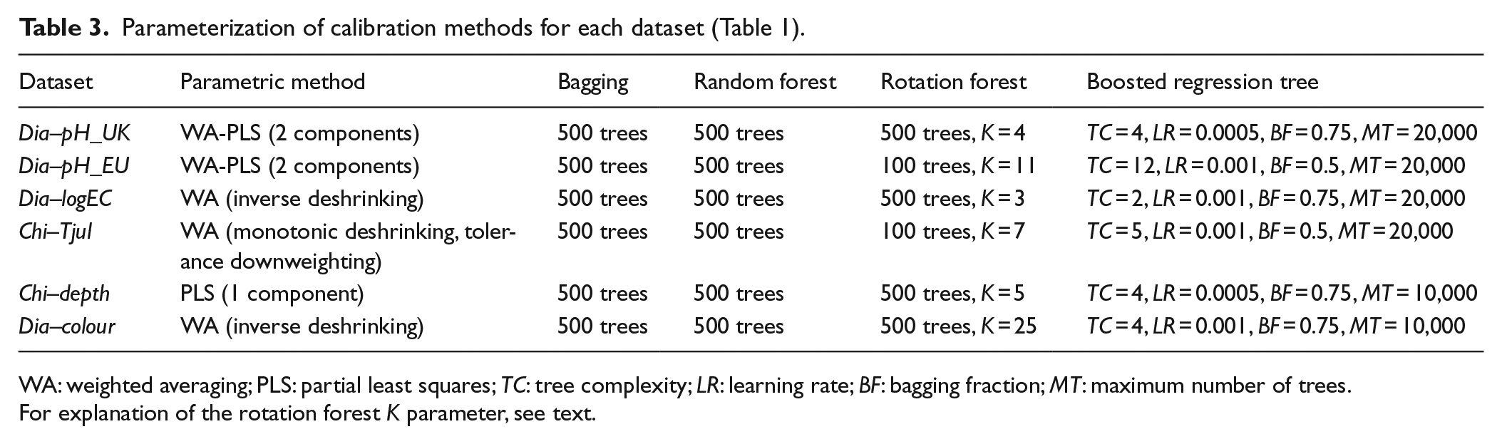
WA: weighted averaging; PLS: partial least squares; TC: tree complexity; LR: learning rate; BF: bagging fraction; MT: maximum number of trees.

For explanation of the rotation forest K parameter, see text.

The effect of RoF parameters on cross-validated RMSEP is plotted in Figure 2. All datasets show an improvement in predictions going from K = 2 to larger values (Figure 2, upper panels), while increasing K starts to eventually hurt performance with all datasets. However, the K giving best CV performance varies with dataset, and no clear relationship is seen between best K and either the number of predictors or the number of samples. Like Kuncheva and Rodríguez (2007), we thus cannot recommend a single value to use. However, we note that the sensitivity of RMSEP to K is not great, and for most datasets used here, any K between 5 and 10 would allow close to optimal performance. While we here mostly used ensembles of 500 trees, the plots of RMSEP as function of L (Figure 2, lower panels) show that with these datasets RMSEP tends to stabilize at a lower L of ca. 50.

Figure 2.

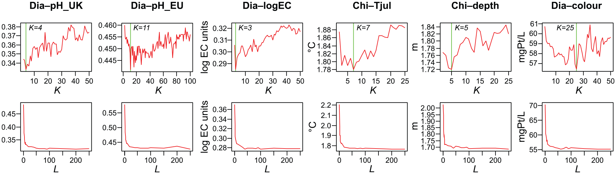
Effect of rotation forest parameters on predictive performance. The upper panels show the effect of K (the number of groups in which the predictor set is passed through principal component analysis) on cross-validated root-mean-square error of prediction (RMSEP) while using ensembles of 10 trees. The K producing the lowest RMSEP is indicated with a vertical line. The lower panels show the effect of L (ensemble size) on RMSEP while using the optimal K. Results are shown for six datasets (see Table 1 for details). All plots are based on running 10 repeats of leave-one-cluster-out (for Chi–depth and Dia–colour) or 10 repeats of 10-fold (for other datasets) cross-validations with each K or L tested, with mean RMSEP reported for each K or L.

Model performance

CV results for the calibration models are presented in Figure 3. With one dataset (Chi–depth), the parametric PLS transfer function (RMSEP = 1.61 m) improves on all tree-ensemble approaches (RMSEP between 1.68 m (RoF) and 1.83 m (BRT)). With the Dia–pH_UK, Dia–pH_EU and Dia–logEC datasets, the parametric transfer function used (WA or WA-PLS) has near-identical performance with the best-performing tree-ensemble approach (either BRT or RaF). With Chi–Tjul and Dia–colour datasets, all tree-ensemble methods improve on the parametric transfer function used (WA). With Dia–colour, the difference between the best tree-ensemble method and WA is quite small (RMSEP = 52.5 mgPt/L with BRT and 57.7 mgPt/L with WA), while a larger difference is found with Chi–Tjul (RMSEP = 1.65°C with RaF and 1.92°C with WA). With Dia–colour, all methods show a relatively poor performance, possibly owing to the relatively weak signal of water colour in the diatom data, as evidenced by the proportion of non-informative taxa in HOF modelling (Table 2). However, for all methods, the cross-validated RMSEP (52.5–57.7 mgPt/L) is smaller than the standard deviation of water colour in the calibration data (65.4 mgPt/L). The diatom–water colour models especially struggle to predict for the samples with high observed water colour values of ⩾200 mgPt/L, with all predicted values falling well below the observations, while for the low end of the water colour gradient (observed values < 200 mgPt/L), especially the best models produce a satisfactory pattern around the 1:1 line in the observed–predicted plots.

Figure 3.

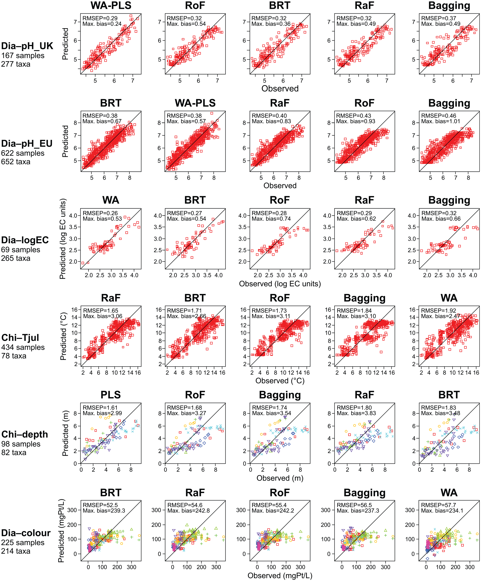
Model performance in cross-validation. The models are shown for each dataset ordered according to increasing root-mean-square error of prediction (RMSEP). Results are shown for six datasets (see Table 1 for details). For each dataset, results are shown using a parametric transfer function (one of partial least squares (PLS), weighted averaging (WA) or weighted averaging-partial least squares (WA-PLS)), bagging, random forest (RaF), rotation forest (RoF) and a boosted regression tree (BRT). Each plot shows the sample-specific predictions versus the observed environmental values. Indicated within each plot are cross-validation performance statistics including the RMSEP and the maximum bias. The cross-validation type used is leave-one-cluster-out for Chi–depth and Dia–colour, while the predictions and performance statistics for the other datasets are the means from 10 runs of 10-fold cross-validation. The sample symbols for Chi–depth and Dia–colour indicate spatial sample cluster membership (see Figure 1).

Results of the complementary h-block CVs for Chi–Tjul are shown in Figure 4. For all calibration methods, RMSEP increases between h = 0 km and h = 200 km, where RMSEP remains constant until h = 500 km. With h larger than 500 km, RMSEP for tree-ensemble techniques increases again, whereas RMSEP of WA with monotonic deshrinking (which is conceptually related to two-component WA-PLS) only starts increasing with h larger than 800 km. The results of h-block CV were as expected for datasets affected by spatial autocorrelation. The increase of RMSEP at short distances of h is indicative of performance estimates affected by spatial autocorrelation. Removing spatially close samples, pseudoreplicates that are not fully independent of the test sample are removed from the training set. As lack of independence increases transfer-function performance (lower RMSEP), removal of spatially close samples leads to increased RMSEP. The increase in RMSEP with large values of h is caused by the reduction in data and thereby information available (Trachsel and Telford, 2015). Between the two distances of h with increasing RMSEP, that is, at h between 200 and 500 km, RMSEP is largely unaffected by h. This region is expected to show unbiased performance estimates, avoiding use of pseudoreplicates but still having enough information to make meaningful inference. The value of h estimated with the method proposed by Telford and Birks (2009) was of 475–525 km (Figure 4) and thereby at the upper end of the lengths of h where RMSEP was not affected by the removal distance. Trachsel and Telford (2015) found that estimates of h obtained using a circular variogram were usually larger than estimates of h obtained using other methods. Hence, h of 475–525 km is certainly conservative. In conclusion, the finding based on 10-fold CV of RaF showing lowest RMSEP for Chi–Tjul is not changed using h-block CV. However, the performance gap between WA and best tree-ensemble methods narrows somewhat in h-block versus 10-fold CV. This is expected, as tree-ensemble methods predict based on a subset of training samples residing in a single terminal tree node, and thus, they benefit more of individual pseudoreplicate samples compared with WA which predicts using taxon responses estimated based on the entire training data.

Figure 4.

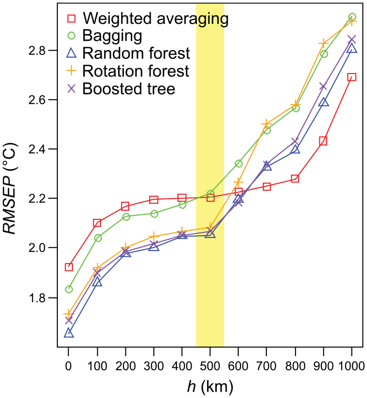
Cross-validated root-mean-square error of prediction (RMSEP) for the dataset Chi–Tjul (see Table 1 for details). Results are shown with h-block cross-validations (Telford and Birks, 2009) using a range of values between 100 and 1000 km for h, while the results for h = 0 km are from a 10-fold cross-validation repeated 10 times. The h value suggested by the test of Telford and Birks (2009) for an unbiased estimate of predictive ability (see text for details) is shown highlighted.

Discussion

This is the first time that different tree-ensemble techniques are compared in fossil proxy calibration, and based on these findings, we can make some generic recommendations about the use of these methods. Among the tree-ensemble approaches tested here, bagging constitutes a baseline algorithm which the other methods build upon. In our results, we find bagging to have the worst performance among tree-ensemble methods for all but one dataset (Chi–depth). A noteworthy feature in the model predictions with bagging are the gaps in the distributions of predictions seen with a number of the datasets, for example, at ca. 6 with Dia-pH_UK, at 2.9–3.4 with Dia–logEC and at ca. 7 and 10°C with Chi–Tjul (Figure 3). Thus, with these datasets, tree building from bootstrap samples does not appear fully sufficient to ensure diverse predictions, and especially with the smallest dataset used (Dia–logEC), the predictions remain clearly semi-discrete. By comparison, these gaps in predictions disappear or become less conspicuous with RaF and RoF (Figure 3) which add further sources of stochasticity into the model building. In view of these results, we cannot recommend the use of bagging in palaeolimnological proxy calibration. By comparison, we find little to choose between RaF, RoF and BRT as they show near-identical performance with most datasets, and each of them has best performance among tree-ensemble methods with at least one dataset. Kuncheva and Rodríguez (2007) tested a number of tree-based algorithms, including bagging, RaF and RoF (but not BRT) in classification, that is, with a categorical response. They ran 10-fold CVs using 32 datasets featuring diverse sample sizes and varying combinations of categorical and continuous predictors. In these classification tests, bagging outperformed RaF with some datasets and had only slightly inferior overall performance. However, Kuncheva and Rodríguez (2007) found RoF to improve considerably on both bagging and RaF.

A distinguishing feature between the tree-ensemble methods are the maximum bias figures, which are lowest for BRT with all but one dataset (Chi–depth). For most models (28 out of 30), the maximum bias value comes from a gradient-end segment, that is, either the first or the last of the 10 segments used for maximum bias calculation. Looking at the predicted–observed plots (Figure 3), the tendency to overestimate for low observed values and underestimate for high observed values is clearly present in all tree-ensemble models. Bias towards dataset mean at gradient ends is an inevitable feature of tree-ensemble predictors, as with gradient-end samples the trees become increasingly likely to predict using samples located towards the centre of the gradient. Based on the maximum bias figures, BRT appears somewhat more robust to this effect, and this is particularly well seen in the gradient-end predictions with Dia–pH_EU where BRT considerably improves on the other tree-ensemble approaches. However, we find parametric transfer functions which, unlike tree ensembles, have some ability to extrapolate beyond the calibration data (Birks et al., 2010), to have the lowest maximum bias with all datasets.

We note three methodological features which set tree ensembles apart from transfer-function approaches such as WA/PLS/WA-PLS and which should be considered in palaeolimnological applications. First, none of the tree-ensemble methods yield exactly the same results with repeated runs (unlike, for example, PLS/WA/WA-PLS) because of the random selection of samples and possibly also predictors during tree building. This causes some instability in the predictions, and also in CV metrics like RMSEP, even in CV schemes using a predetermined division of samples into test and training sets (LOO, h-block, LOCO) instead of a randomized grouping (k-fold). However, in 10 repeated runs of the LOCO CV using Chi–depth, we found relatively small ranges of variation in RMSEP with bagging (1.73–1.75 m), RaF (1.77–1.83 m), RoF (1.68–1.70 m) and BRT (1.80–1.85 m), supporting our conclusions about the relative performance of the methods. With Dia–colour, the relative variation in RMSEP was smaller than with Chi–depth with all tree-ensemble methods, so it appears that the individual trees became more stable with the larger dataset. Second, tree ensembles are not affected by commonly used species-data transformations, as the individual tree splits are determined by the rank order for each predictor, and this order is preserved in monotonic transformations such as the square-root transformation (De’ath and Fabricius, 2000). Third, all predictor variables need not be continuous (e.g. taxon percentages), but any mixture of continuous, binary and categorical predictor variables can be employed (Elith et al., 2008). This could be useful in incorporating non-continuous supplementary variables (e.g. observations of botanical macroremains) in environmental reconstructions (see Salonen et al. (2014) for further discussion). Likewise, the response (environmental) variable can be binary or categorical instead of continuous (De’ath and Fabricius, 2000).

A striking feature in our results is the inability of tree ensembles to compete with a simple, one-component PLS transfer function with Chi–depth. We suggest three possible contributors to this. First, many of the most abundant chironomid taxa show a strong, linear or otherwise monotonic responses to water depth (Engels and Cwynar, 2011; Table 1), and such relative absence of nonlinearities or interactions would diminish many of the intrinsic advantages of tree-based modelling while linearity (as in PLS) may prove an adequate approximation (De’ath and Fabricius, 2000; Schonlau, 2005). Second, this dataset is one of the smallest used here, and especially with one cluster omitted in LOCO CV, the data may become sparse enough to disadvantage tree-based methods, which base each prediction on a small subset of samples residing in a terminal tree node and thus require densely sampled calibration data to populate the gradient evenly with terminal nodes for accurate prediction (Hjort and Marmion, 2008; Wisz et al., 2008). By comparison, a method such as PLS or WA/WA-PLS which estimates taxon responses using the entire training set may prove more robust to gaps in gradient sampling. This is also a possible explanation for the superior performance of WA compared with tree-ensemble methods with large values of h (>500 km) in h-block CV (Figure 4) for the Chi–Tjul dataset, where the performance of all methods starts to weaken because of poor sampling of the gradient, but WA suffers considerably less and starts to outperform all tree-ensemble approaches by h = 700 km. Third, the water-depth signal appears to be strong in the chironomid data, as a comparatively small proportion of taxa shows no significant response in HOF modelling. By contrast, we find all tree-ensemble methods to improve on WA with Dia–colour, the dataset with the largest proportion of non-informative taxa (Table 1). A high number of non-informative taxa might favour the tree-based models which are inherently selective in identifying and employing the best indicator taxa while ignoring taxa which have no indicator value (Juggins et al., 2015).

Conclusion

In practice, a proxy-calibration method must often be chosen without access to fully independent test sets, and assessing the relative strengths of different methods can be challenging (Juggins and Birks, 2012; Trachsel and Telford, 2015). Thus, it would be useful to identify guidelines for recognizing calibration scenarios (e.g. dataset size, distribution of response shapes or the relative influence of the reconstructed variable) which might favour a specific method family, such as parametric transfer functions or a tree-based approach. Here, we have shown that tree-ensemble methods can in some cases outperform a generally robust transfer-function technique, especially with larger datasets characterized by complex and diverse taxon responses and abundant noise. However, parametric transfer functions often show near-equal performance or even improve on tree ensembles, particularly with smaller datasets and data characterized by strong, linear species responses. Considering this pattern, it seems prudent to expand the testing of tree-ensemble approaches to even larger and more complex calibration datasets, such as the continental-scale pollen–climate datasets commonly used in palaeoclimate studies. We encourage researchers to further test these methods using a range of new proxy datasets representing different taxa, environments and spatio-temporal scales; to explore the potential and limitations of these methods; and to identify scenarios and applications where they may prove especially useful.

Footnotes

Acknowledgements

SE is grateful to Les C Cwynar for support in producing the Massachusetts chironomid data. We thank Andrew Scott Medeiros, Keely Mills and Jan Weckström for their help in acquiring data for this study.

Funding

This work was funded by the Academy of Finland programme on long-term environmental changes (project no. 278692). JSS acknowledges additional funding from the Finnish Cultural Foundation. AJV is supported by a Canadian Institute for Health Research (CIHR) grant (MOP-97939) and MT by the Norwegian Research Council FriMedBio project palaeoDrivers (213607).

References

Battarbee

Flower

Juggins

. (1997) The relationship between diatoms and surface water quality in the Høylandet area of Nord-Trøndelag, Norway. Hydrobiologia 348: 69–80.

Birks

HJB

Heiri

Seppä

. (2010) Strengths and weaknesses of quantitative climate reconstructions based on late-Quaternary biological proxies. The Open Ecology Journal 3: 68–110.

Birks

HJB

Juggins

Line

(1990a) Lake surface-water chemistry reconstructions from palaeolimnological data. In: Mason

(ed.) The Surface Waters Acidification Programme. Cambridge: Cambridge University Press, pp. 301–313.

Birks

HJB

Line

Juggins

. (1990b) Diatoms and pH reconstruction. Philosophical Transactions of the Royal Society of London, Series B: Biological Sciences 327: 263–278.

Breiman

(1996) Bagging predictors. Machine Learning 24: 123–140.

Breiman

(2001) Random forests. Machine Learning 45: 5–32.

De’ath

(2007) Boosted trees for ecological modeling and prediction. Ecology 88: 243–251.

De’ath

Fabricius

(2000) Classification and regression trees: A powerful yet simple technique for ecological data analysis. Ecology 81: 3178–3192.

Elith

Graham

Anderson

(2006) Novel methods improve prediction of species’ distributions from occurrence data. Ecography 29: 129–151.

10.

Elith

Leathwick

Hastie

(2008) A working guide to boosted regression trees. Journal of Animal Ecology 77: 802–813.

11.

Engels

Cwynar

(2011) Changes in fossil chironomid remains along a depth gradient: Evidence for common faunal thresholds within lakes. Hydrobiologia 665: 15–38.

12.

Engels

Cwynar

Rees

ABH

. (2012) Chironomid-based water depth reconstructions: An independent evaluation of site-specific and local inference models. Journal of Paleolimnology 48: 693–709.

13.

Felde

Bjune

Grytnes

J-A

. (2014) A comparison of novel and traditional numerical methods for the analysis of modern pollen assemblages from major vegetation–landform types. Review of Palaeobotany and Palynology 210: 22–36.

14.

Fortin

M-C

Medeiros

Gajewski

. (2015) Chironomid-environment relations in northern North America. Journal of Paleolimnology 54: 223–237.

15.

Goring

Lacourse

Pellatt

. (2010) Are pollen-based climate models improved by combining surface samples from soil and lacustrine substrates. Review of Palaeobotany and Palynology 162: 203–212.

16.

Hjort

Marmion

(2008) Effects of sample size on the accuracy of geomorphological models. Geomorphology 102: 341–350.

17.

Huisman

Olff

Fresco

LFM

(1993) A hierarchical set of models for species response analysis. Journal of Vegetation Science 4: 37–46.

18.

Jansen

Oksanen

(2013) How to model species responses along ecological gradients – Huisman-Olff-Fresco models revisited. Journal of Vegetation Science 24: 1108–1117.

19.

Juggins

(2013a). Quantitative reconstructions in palaeolimnology: New paradigm or sick science? Quaternary Science Reviews 64: 20–32.

20.

Juggins

(2013b) rioja: Analysis of Quaternary science data. Available at: https://cran.r-project.org/web/packages/rioja/index.html (accessed 22 February 2016).

21.

Juggins

Birks

HJB

(2012) Quantitative environmental reconstructions from biological data. In: Birks

HJB

Lotter

Juggins

. (eds) Tracking Environmental Change using Lake Sediments, Vol. 5: Data Handling and Numerical Techniques. Dordrecht: Springer, pp. 431–494.

22.

Juggins

Simpson

Telford

(2015) Taxon selection using statistical learning techniques to improve transfer function prediction. The Holocene 25: 130–136.

23.

Kuncheva

Rodríguez

(2007) An experimental study on rotation forest ensembles. In: Haindl

Kittler

Roli

(eds) Multiple Classifier Systems. Berlin: Springer, pp. 459–468.

24.

Lepš

Šmilauer

(2003) Multivariate Analysis of Ecological Data using CANOCO. Cambridge: Cambridge University Press, 269 pp.

25.

le Roux

Lenoir

Pelissier

. (2013) Horizontal, but not vertical, biotic interactions affect fine-scale plant distribution patterns in a low energy system. Ecology 94: 671–682.

26.

Zheng

. (2015) Assessing the importance of climate variables for the spatial distribution of modern pollen data in China. Quaternary Research 83: 289–297.

27.

Liaw

Wiener

(2002) Classification and regression by randomForest. R News 2(3): 18–22.

28.

Mills

Ryves

(2012) Diatom-based models for inferring past water chemistry in western Ugandan crater lakes. Journal of Paleolimnology 48: 383–399.

29.

Pajunen

Luoto

Soininen

(2016) Climate is an important driver for stream diatom distributions. Global Ecology and Biogeography. 25: 198–206.

30.

R Core Team (2014) R: A Language and Environment for Statistical Computing. Vienna: R Foundation for Statistical Computing. Available at: http://www.R-project.org/.

31.

Ridgeway

(2013) gbm: Generalized boosted regression models. R package version 2.1. Available at: http://CRAN.R-project.org/package=gbm (27 January 2015).

32.

Rodríguez

Kuncheva

Alonso

(2006) Rotation forest: A new classifier ensemble method. IEEE Transactions on Pattern Analysis and Machine Intelligence 28: 1619–1630.

33.

Salonen

Luoto

Alenius

. (2014) Reconstructing palaeoclimatic variables from fossil pollen using boosted regression trees: Comparison and synthesis with other quantitative reconstruction methods. Quaternary Science Reviews 88: 69–81.

34.

Salonen

Seppä

Luoto

. (2012) A North European pollen–climate calibration set: Analysing the climatic responses of a biological proxy using novel regression tree methods. Quaternary Science Reviews 45: 95–110.

35.

Schonlau

(2005) Boosted regression (boosting): An introductory tutorial and a Stata plugin. The Stata Journal 5: 330–354.

36.

Simpson

Birks

(2012) Statistical learning in palaeolimnology. In: Birks

HJB

Lotter

Juggins

. (eds) Tracking Environmental Change using Lake Sediments: Data Handling and Numerical Techniques. Dordrecht: Springer, pp. 249–327.

37.

Soininen

Paavola

Muotka

(2004) Benthic diatom communities in boreal streams: Community structure in relation to environmental and spatial gradients. Ecography 27: 330–342.

38.

Steinberg

(2003) Ecology of Humic Substances in Freshwaters: Determinants from Geochemistry to Ecological Niches. Berlin: Springer.

39.

Stevenson

Juggins

Birks

HJB

. (1991) The Surface Waters Acidification Project Palaeolimnology Programme: Modern Diatom/Lake-Water Chemistry Data-Set. London: ENSIS.

40.

Telford

Birks

HJB

(2009) Evaluation of transfer functions in spatially structured environments. Quaternary Science Reviews 28: 1309–1316.

41.

Telford

Birks

HJB

(2011) A novel method for assessing the statistical significance of quantitative reconstructions inferred from biotic assemblages. Quaternary Science Reviews 30: 1272–1278.

42.

ter Braak

CJF

Juggins

(1993) Weighted averaging partial least squares regression (WA-PLS): An improved method for reconstructing environmental variables from species assemblages. Hydrobiologia 269–270: 485–502.

43.

Therneau

Atkinson

Ripley

(2014) Recursive partitioning and regression trees. Available at: http://cran.r-project.org/web/packages/rpart/index.html (12 January 2015).

44.

Trachsel

Telford

(2015) Technical Note: Estimating unbiased transfer-function performances in spatially structured environments. Climate of the Past Discussions 11: 4729–4749.

45.

van der Voet

(1994) Comparing the predictive accuracy of models using a simple randomization test. Chemometrics and Intelligent Laboratory Systems 25: 313–323.

46.

Veloz

Williams

Blois

. (2012) No-analog climates and shifting realized niches during the late quaternary: Implications for 21st-century predictions by species distribution models. Global Change Biology 18: 1698–1713.

47.

Wenger

Olden

(2012) Assessing transferability of ecological models: An underappreciated aspect of statistical validation. Methods in Ecology and Evolution 3: 260–267.

48.

Wisz

Hijmans

. (2008) Effects of sample size on the performance of species distribution models. Diversity and Distributions 14: 763–773.

49.

Zhao

Liu

. (2012) Application and limitations of the Artemisia/Chenopodiaceae pollen ratio in arid and semi-arid China. The Holocene 22: 1385–1392.

50.

Zimmermann

Edwards

Graham

. (2010) New trends in species distribution modelling. Ecography 33: 985–989.