Millennial to secular time-scale impacts of climate and sea-level changes on mangroves from the Doce River delta,Southeastern Brazil

Abstract

This work integrates geomorphological, sedimentological, and palynological data with radiocarbon dating, as well as δ¹³C, δ¹⁵N, and C/N from sedimentary organic matter to provide a model of mangrove dynamics during the evolution of a wave-dominated delta in Southeastern Brazil. Mangrove dynamics are analyzed within the context of millennial and secular climatic and sea-level changes. Tidal flats, positioned at highest limit of the intertidal zone along the edge of a lagoon sheltered by beach ridges, were occupied by wetlands represented by mangrove and herbaceous vegetation during the mid-Holocene high sea level. After considering the relative sea-level fall and relatively higher fluvial sediment discharge, during the last ~6350 years, progradation took place along this shoreline, resulting in extensive beach ridge deposits that overlie transgressive muds. This process led to loss of mangrove area. Similar dynamics were repeated at ~3043 cal. yr BP, although in a relatively more distal (i.e. seaward) position. Between ~1337 and ~900 cal. yr BP, a tidal flat attached to the edge of a lagoon near the modern coastline was colonized by herbaceous vegetation (C4 plants). The next phase, which occurred between ~900 and ~400 or ~100 cal. yr BP, is marked by the transition from herbaceous to mangrove tidal flats with an increased trend of terrestrial organic matter. During the recent centuries, a mangrove vegetation became established, and there was an increased trend of estuarine-derived organic matter. This mangrove phase, recorded during the last century(ies), may be due to a relative sea-level rise. Under this scenario, erosion of beach ridges and expansion of lagoons and mangroves are expected along the littoral of the State of Espírito Santo in Southeastern Brazil.

Keywords

facies association Holocene isotopes mangrove palynology sea level

Introduction

Today, there is great concern about how mangroves will respond to changes in temperature, CO₂, rainfall, storms, and sea-level rise (Blasco et al., 1996; Duke et al., 2007; McLeod and Salm, 2006; Masselink and Gehrels, 2014). The ecosystem products and services provided by mangrove forests are well understood and include the protection of coasts from erosion (Ewel et al., 1998), sources and sinks of organic carbon (Dittmar et al., 2006), sediments (Walsh and Nittrouer, 2004), and plant and animal productivity (Ewel et al., 1998). Another important aspect related to mangrove forests and global climate change is the role of these systems in the carbon sequestration and storage (Alongi, 2014; Donato et al., 2011; Giri et al., 2011). Despite mangroves being among the most carbon-rich biomes, containing an average of 937 tC ha⁻¹ (Alongi, 2012), they represent only 0.5% of the coastal habits to carbon sequestration in the global coastal ocean (Alongi, 2014). The global carbon sequestration induced by mangroves (13.5 Gt yr⁻¹) may compensate about 1% of carbon sequestration by the world’s forests; however, as coastal habitats, they account for 14% of carbon sequestration by the global ocean (Alongi, 2012).

It is important to note that the Brazilian coast contains the world’s third largest unitary mangrove region, estimated to cover a total area of 962,683 ha (Giri et al., 2011), along a coastline of approximately 7637 km (Schaeffer-Novelli et al., 1990).

However, global mangrove distributions have fluctuated throughout geological and human history due to climatic changes and sea-level oscillations (Alongi, 2008; Cohen et al., 2012; Fromard et al., 2004). Regarding the Brazilian littoral, post-glacial sea-level rise and changes in fluvial discharges are considered the main driving forces to the mangrove expansion or contraction phases (Cohen et al., 2012, 2014), although tectonics might have played a role in this geological setting (Miranda et al., 2009; Rossetti and Valeriano, 2007) at least during the Holocene.

Considering Holocene sea-level changes, it appears to have crossed the present level around 7000 yr BP, reaching 4–6 m above the present one in many areas of the Brazilian coast (Angulo et al., 2006; Martin and Suguio, 1992; Reis et al., 2013; Rossetti et al., 2008), as well as other areas of the South American coast (Milne et al., 2005). Globally, over the last 1000 years, the minimum sea level (−19 to −26 cm) occurred around AD 1730 and the maximum sea level (12–21 cm) around AD 1150 (Grinsted et al., 2009). A similar sea-level trend was recorded along the northern Brazilian littoral, which had significant impact on mangrove dynamics (Cohen et al., 2005a, 2005b). The combination of paleo sea-level data and long-tide gauge records confirms that the rate of rise has increased from low rates of change during the late-Holocene (order of tenths of millimeter per year) to rates of almost 2 mm yr⁻¹ averaged over the 20th century, with a likely continuing acceleration during the 20th century (Church et al., 2013). The relative sea-level (RSL) rise has caused a mangrove retraction along the northern Brazilian littoral. The loss of mangrove area is mainly due to the erosion and landward sand migration, which covers the mudflat and asphyxiates the vegetation (Cohen et al., 2009; Cohen and Lara, 2003; França et al., 2012).

Regarding the littoral of the State of Espírito Santo in Southeastern Brazil, the nonequilibrium between fluvial sediment supply and RSL changes during the Pleistocene (Cohen et al., 2014; Rossetti et al., 2015), and Holocene (Buso Junior et al., 2013; França et al., 2013, 2015) has significantly affected the depositional systems and created and destroyed areas suitable to mangrove development (Castro et al., 2013; França et al., 2013).

In order to propose a model to explain the relationship between the evolution of beach ridges, formed during the development of deltaic systems, and mangrove dynamics according to climate and sea-level changes, this work emphasizes the late-Holocene deposits of the Doce River delta plain, mainly those formed in the last 1300 years BP. The interpretations are based on the characterization of geomorphology, sedimentology, palynology, and bulk sedimentary organic matter through δ¹³C, δ¹⁵N, and C/N analyses of sediment cores from a coastal plain occupied by mangrove and herbaceous vegetation and temporally dated with ¹⁴C dating.

Modern settings

Study area and geological setting

The study site is located on the Doce River delta, State of Espírito Santo, Southeastern Brazil (Figure 1), about 60 km from the mouth of the Doce River. The Holocene sedimentary history in this sector is strongly controlled by RSL changes, fluvial supply, and longshore transport (Cohen et al., 2014). The study area is composed of a Miocene age plateau represented by continental deposits of the Barreiras Formation, which are slightly sloping seaward. This site is characterized by many wide valleys with flat bottoms where silty deposits were accumulated during the Quaternary (Martin et al., 1996). The study area is part of a larger area of tectonically stable Precambrian crystalline rocks. Four geomorphological units are recognized in this area: (1) a mountainous province constituted by Precambrian rocks having a multidirectional rectangular dendritic drainage network; (2) a seaward gently slopping tableland consisting of fluvial, alluvial fan and probably also marine transgressive siliciclastic deposits of the Neogene Barreiras Formation (Arai, 2006; Dominguez et al., 2009); (3) a coastal plain area, with fluvial, transitional, and shallow marine sediments deposited during RSL changes (Martin and Suguio, 1992); and (4) an inner continental shelf area (Asmus et al., 1971).

Figure 1.

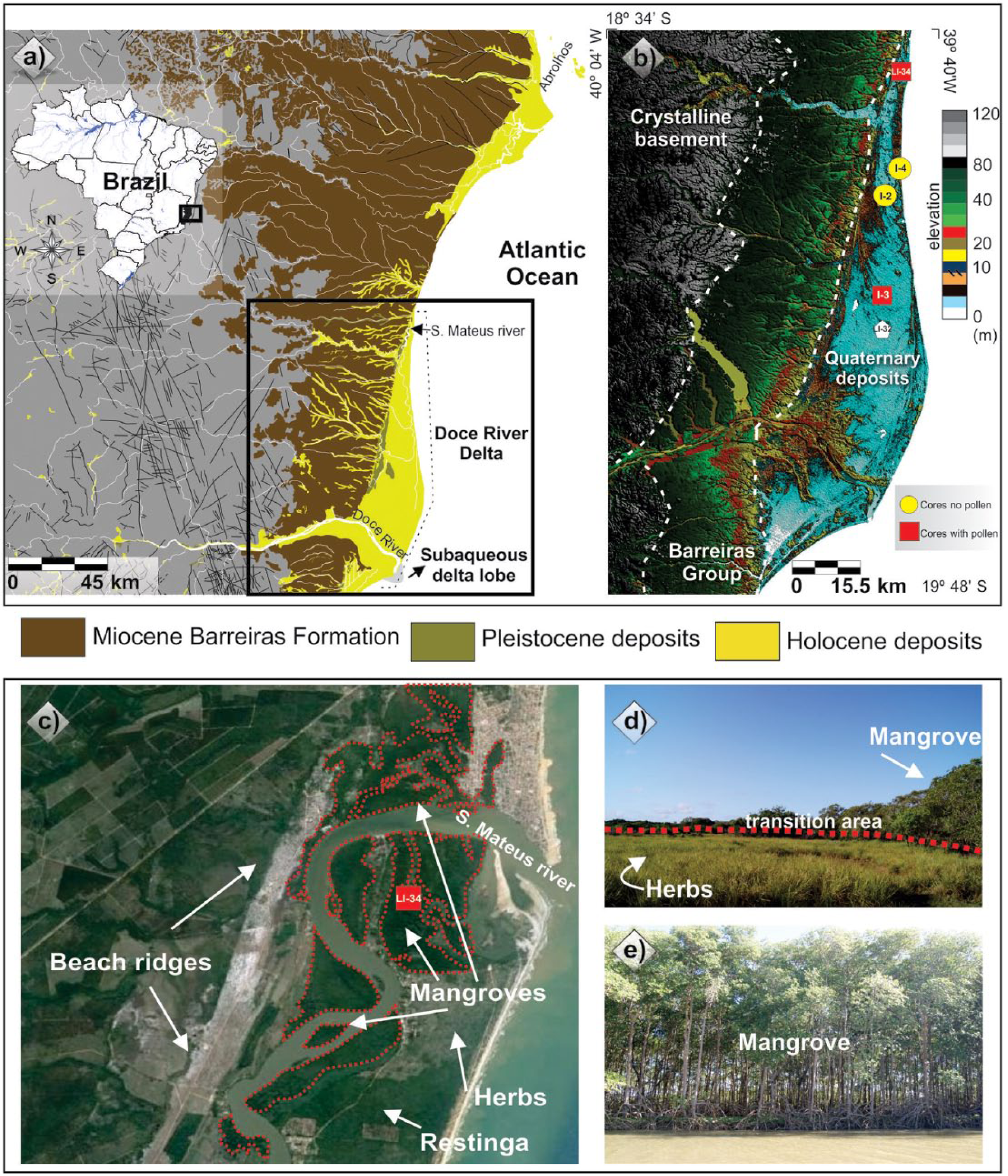
Location of the study area: (a) Miocene Barreiras Formation, Pleistocene and Holocene deposits, and the Doce River delta; (b) topographic profile obtained from the digital elevation model – SRTM, illustrating a large area slightly more depressed on the Doce River delta plain; (c) satellite image with beach ridges, herbaceous plain, and mangroves developed in the Holocene; (d) the contact between mangrove and herbaceous vegetation; and (e) the mangrove ecosystem.

Modern climate

The region is characterized by a warm and humid tropical climate with annual precipitation averaging 1400 mm (Peixoto and Gentry, 1990). Higher precipitation generally occurs in the summer, with a dry fall-winter season controlled by the position of both the Intertropical Convergence Zone (ITCZ) and the South Atlantic Convergence Zone (SACZ; Carvalho et al., 2004). The area is entirely located within the South Atlantic trade wind belt (NE-E-SE). This is related to a local high-pressure cell and the periodic advance of the Atlantic Polar Front during the autumn and winter, which generates SSE winds (Dominguez et al., 1992; Martin et al., 1998). The rainy season occurs between the months of November and January, with a drier period between May and September. The average temperature ranges between 20°C and 26°C.

Modern vegetation

Wetlands cover a significant part of the study site, with mangrove trees being 5–15 m in height. Important species, such as Rhizophora mangle and Laguncularia racemosa, occur near lagoon margins, while Avicennia germinans grows mainly on higher topographic elevations. The mangrove ecosystem is currently restricted to the northern littoral of the coastal plain (Bernini et al., 2006). Ipomoea pes-caprae, Hancornia speciosa, Chrysobalanus icaco, Hirtella Americana, Cereus fernambucensis, and palm trees characterize the sandy coastal plain, as well as orchids and bromeliads that grow on the trunks and branches of larger trees. Tropical rainforest occurs naturally on higher terrains, where the most representative plant families are Annonaceae, Fabaceae, Myrtaceae, Sapotaceae, Bignoniaceae, Lauraceae, Hippocrateaceae, Euphorbiaceae, and Apocynaceae (Peixoto and Gentry, 1990). The coastal plain between São Mateus and Doce River is characterized by freshwater species, such as Hypolytrum sp. and Panicum sp., and brackish or marine water species, such as Polygala cyparissias, Remiria maritima, Typha sp., Cyperus sp., Montrichardia sp., Tapirira guianensis, and Symphonia globulifera. Herbaceous vegetation dominates the sampling site, being represented by Araceae, Cyperaceae, and Poaceae, with some trees and shrubs on the plain’s edge.

Materials and methods

Remote sensing

The mapping of detectable vegetation contrasts for the study area was based on analysis of freely available remote sensing data. A LANDSAT optical images acquired on April 2013 and January 1984 were obtained from National Institute of Space Research (INPE, Brazil) and United States Geological Survey (USGS) global archive (Woodcock et al., 2008). These optical images have a level 1 terrain (L1T) processing, meaning that the data had been radiometrically and geometrically corrected and orthorectified. A three-color band composition (red, green, blue, 543) image was created and processed using the SPRING 4.3.3 package to discriminate the geomorphological features of interest.

Further processing included the following:

Digitalization of individual images showing vegetation boundaries and posterior layer overlap using georeferenced points to develop a time series. Image texture, object size, and shape features allowed a clear delimitation of the dense mangrove areas, due to the contrast with other adjacent vegetation types.

Sample synthetic color images (2015, CNES/ASTRIUM) available from Google Earth (Yu and Gong, 2011) were used as a reference to characterize vegetation classes. These images present higher resolution than the LANDSAT images used in the temporal spatial analysis.

Topographic data were derived from SRTM − 30-m digital elevation model, downloaded from the USGS Seamless Data Distribution System (http://earthexplorer.usgs.gov/). Image interpretation of elevation data was carried out using the Global Mapper 12 software.

Selection of areas for field validation of satellite images and more detailed evaluation of changes in vegetation coverage. A total of 10 sites were checked to validate the classification of vegetation cover derived from satellite image analyses. The transition mangrove or herbaceous and mangrove or restinga vegetation were chosen for the fieldwork.

Fieldwork

The fieldwork was carried out in July 2011, September 2013, and August 2015. The 4-m-deep sediment core LI-34 (18°36′27.4″S or 39°44′40.4″W, 2 m elevation) was taken on a mangrove tidal mudflat, while the 7.5-m-deep I-2 (18°51.1″S or 39°48.6′W, 6 m elevation), 9-m-deep I-3 (19°03′13.6″S or 39°46′55″W, 5 m elevation), and 5-m-deep I-4 (19°04′28″S or 39°43′21″W, 5 m elevation) cores were taken from a restinga vegetation, using a Russian sampler (Cohen, 2003; Figure 1). The core Li-32 (França et al., 2013) has been correlated with the new cores due to its more proximal position (Figure 2), which records the early- to mid-Holocene marine transgression followed by the mid-Holocene to late-Holocene marine regression in the study area (França et al., 2013).

Figure 2.

Correlation of facies associations identified in the studied cores.

Visual observation and photographic documentation were used to determine the main geobotanical units. Porewater salinities of surface (0–10 cm) of tidal flats were determined in the field by a refractometer. The geographical positions of cores were determined by global positioning system (GPS) using the SAD69 as reference datum. The study site presents a tidal range of 1.5 m (Departamento de Hidrografia e Navegação, 2014).

Facies description

The cores were submitted to x-rays in order to identify the sedimentary features. They were transported to the Laboratory of Chemical Oceanography, Federal University of Pará (UFPA), where sediment grain sizes were determined using a SHIMADZU SALD 2101 laser diffraction particle size analyzer, and the graphics were obtained using the Sysgran program (Camargo, 1999). The sediment grain size distribution follows the grain size scale of Wentworth (1922), with sand (2–0.0625 mm), silt (62.5–3.9 µm), and clay fractions (3.9–0.12 µm). Following proposals of Harper (1984) and Walker and James (1992), facies analysis included description of color (Munsell Color, 2009), lithology, texture, and structure. The sedimentary facies were codified following Miall (1978).

Palynological analysis

For pollen analysis, 1-cm³ samples were taken at 10-cm intervals along the core LI-34 and between 9 and 6 m depth in the core I-3. All samples were prepared using standard pollen analytical techniques including acetolysis (Faegri and Iversen, 1989). Sample residues were mounted on slides in a glycerin gelatin medium. Pollen and spores were identified by comparison with reference collections of about 4000 Brazilian forest taxa and various pollen keys (Absy, 1975; Colinvaux et al., 1999; Markgraf and D’Antoni, 1978; Roubik and Moreno, 1991; Salgado-Labouriau, 1997), jointly with the reference collection of the Laboratory of Coastal Dynamics – UFPA and ¹⁴C Laboratory of the Center for Nuclear Energy in Agriculture (CENA/USP). A minimum of 300 pollen grains were counted for each sample. Pollen results for cores I-2 and I-4 are not presented due to the low concentration of grains. The total pollen sum excludes fern spores, algae, and foraminiferal tests. Pollen and spore data are presented in pollen diagrams as percentages of the total pollen sum. The taxa were grouped according to source: mangroves, trees and shrubs, palms, and herbs pollen. The software TILIA and TILIAGRAPH were used for calculation and plotting of pollen diagrams (Grimm, 1990). CONISS was used for cluster analysis of pollen taxa, which allowed the zonation of the pollen diagrams (Grimm, 1987).

Isotopic and chemical analysis

Samples (6–50 mg) were collected at 10-cm intervals only in core LI-34 due to its high organic matter preservation and muddy nature. Sediments were treated with 4% HCl to eliminate carbonates, washed with distilled water until the pH reached 6, dried at 50°C, and finally homogenized. These samples were analyzed for total organic carbon (TOC) and total nitrogen (TN), a process that was carried out at the Stable Isotope Laboratory of the CENA/USP. The results are expressed as percentages of dry weight, with analytical precision of 0.09% (TOC) and 0.07% (TN), respectively. The ¹³C and ¹⁵N results are expressed as δ¹³C and δ¹⁵N with respect to Vienna Pee Dee Belemnite (VPDB) standard and atmospheric air, using the following notation:

\begin{matrix} δ^{13} C (‰) = [(\frac{R_{1 sample}}{R_{2 standard}}) - 1] 1000 \\ δ^{15} N (‰) = [(\frac{R_{3 sample}}{R_{4 standard}}) - 1] 1000 \end{matrix}

where R_1sample and R_2standard are the ¹³C/¹²C ratio of the sample and standard, and R_3sample and R_4standard are the ¹⁵N/¹⁴N ratio of the sample and standard, respectively. Analytical precision is ±0.2‰ (Pessenda et al., 2004).

The organic matter source dependent of the environment, with different δ¹³C, δ¹⁵N, and C/N compositions (e.g. Lamb et al., 2006), is as follows: The C3 terrestrial plants, mainly represented by trees and shrubs, shows δ¹³C values between −32‰ and −21‰ and C/N ratio > 12, while C4 plants, mainly represented by herbs, have δ¹³C values ranging from −17‰ to −9‰ and C/N ratio > 20 (Deines, 1980; Meyers, 1997). Freshwater algae have δ¹³C values between −25‰ and −30‰ (Meyers, 1997; Schidlowski et al., 1983) and marine algae around −24‰ to −16‰ (Meyers, 1997). The plants of aquatic environments normally use dissolved inorganic nitrogen, which is isotopically enriched in ¹⁵N by 7–10‰ relative to atmospheric N (0‰); thus, terrestrial plants that use N₂ derived from the atmosphere have δ¹⁵N values ranging from 0‰ to 2‰ (Meyers, 2003; Thornton and McManus, 1994). The binary analysis between δ¹³C versus C/N was used to interpret sources of organic matter (Lamb et al., 2006; Meyers, 2003; Wilson et al., 2005).

Radiocarbon dating

Based on stratigraphic discontinuities that suggest changes in the tidal inundation regime, nine bulk samples (10 g each) were selected for radiocarbon analysis. In order to avoid natural contamination by shell fragments, roots, seeds, and so on (e.g. Goh, 2006), the sediment samples were checked and physically cleaned under the stereomicroscope. The organic matter was chemically treated to remove younger organic fractions (i.e. fulvic and/or humic acids) and eliminate adsorbed carbonates. This was achieved by placing the samples in 2% HCl at 60°C for 4 h, followed by rinses with distilled water to neutralize the pH. The samples were dried at 50°C. A detailed description of the chemical treatment for sediment samples can be found in Pessenda et al. (2010, 2012). Radiocarbon dating for the sedimentary succession was provided by accelerator mass spectrometry (AMS). Samples were analyzed at the Radiocarbon Laboratory of the Universidade Federal Fluminense (LAC-UFF) and Center for Applied Isotope Studies, University of Georgia (UGAMS), which received the purified CO₂ in evacuated glass ampoules prepared at the ¹⁴C Laboratory of CENA/USP. Radiocarbon ages were normalized to a δ¹³C of −25‰ VPDB and reported as calibrated years (calibrated years before the present; 2σ) using CALIB 6.0 (Reimer et al., 2009). The dates are reported in the text as the median of the range of calibrated ages (Table 1).

Table 1.

Sediment samples selected for radiocarbon dating and results (Doce River delta) with code site, laboratory number, depth, material, ¹⁴C yr BP, and calibrated ages and median of calibrated ages, and sedimentation rates.

Code site and laboratory number	Core	Depth (m)	Material	Ages (¹⁴C yr BP, 1σ)	Ages (cal. yr BP, 2σ)	Median of age range (cal. yr BP)	Sedimentation rates (mm yr⁻¹)
LACUFF 140157	I-2	5.6	Bulk sedimentation	2092 ± 47	1933–2156	2040	2.6
LACUFF 140156	I-2	7.8	Bulk sedimentation	4708 ± 63	5318–5492	5400	0.65
LACUFF140142	I-3	2.62–2.63	Bulk sedimentation	2754 ± 60	2753–2980	2860	0.90
LACUFF140143	I-3	5.85–5.88	Bulk sedimentation	5571 ± 30	6301–6405	6350	0.92
LACUFF140144	I-3	8.04–8.09	Bulk sedimentation	5604 ± 31	6309–6442	6370	109.5
LACUFF13021	LI-34	0.60–0.64	Bulk sedimentation	338 ± 43	307–409	358	1.5
LACUFF13022	LI-34	1.35–1.40	Bulk sedimentation	195 ± 37	105–114	110	–
UGAMS15848	LI-34	2.60–2.63	Bulk sedimentation	1200 ± 25	1210–1227	1219	2.3
UGAMS15849	LI-34	3.72–3.75	Bulk sedimentation	1440 ± 25	1299–1375	1337	9.5

Results

Geomorphology and vegetation

Five geomorphological units characterize the Doce River delta plain: (1) beach ridges or spits, (2) fluvial and distributary channels, (3) interdistributary bays, (4) transgressive (estuarine, lagoonal, and embayment) environments, and (5) fluvial terraces (Rossetti et al., 2015). Regarding the sampling sites and the objective of this work, only beach ridges were described based on satellite images. In the study site, beach ridges form elongated, narrow, and convex-upward morphologies positioned parallel to nearly parallel to coastline. In the field, beach ridges present undulating reliefs and on depressions, in the proximal portion of the delta plain, freshwater marshes mainly represented by herbs with some palms and shrubs occur. A gradual transition occurs toward the distal portion of the delta plain close to the shoreline, which presents many coastal sand barriers parallel to the shore and sometimes are separated from the mainland by lagoons. This geomorphological unit is colonized by ‘restinga’ vegetation. It is mainly dominated by palm trees as well as Ipomoea pes-caprae, Hancornia speciosa, Chrysobalanus icaco, Hirtella Americana, Cereus fernambucensis, and Anacardium occidentale.

The studied lagoon presents muddy tidal flats with smooth gradients dissected by creeks that enable the tidal influence on inner zones. The tidal flats exhibit porewater salinity gradients (30–80‰) that reflect on vegetation zones. Herbaceous vegetation, dominated by Cyperaceae and Poaceae (only those tolerate salinity species), occurs generally in the inner part of muddy tidal flats, and it is flooded only by the highest spring tides because it occupies surfaces topographically higher than mangroves, mainly represented by Rhizophora, Avicennia, and Laguncularia in the mid-tide mark. The limits between mangrove, restinga, and herbaceous vegetation are always clearly fixed because the transition between these vegetation units causes a spectral response easily distinguishable in color band composition of satellite images. During the fieldwork, it was possible to confirm these vegetation units (Figure 1).

In the study site, usually, the transition restinga or mangrove (Figure 1d) occurs abruptly by a topographical difference. These locations present erosion of highest surface and subsequent sedimentation in an appropriate lower level to the tidal influence and mangrove development. Thus, in this situation, the mangrove expansion occurs by erosion of substrate adjacent to tidal flat. However, at the sampling site of the core Li-34, the mangrove or herbaceous vegetation transitions are smooth. This suggests that mangrove migration to higher surfaces may take place by a rise in the tidal limits.

Radiocarbon dating

The ages, shown in Table 1, indicate sediment deposition during the mid-Holocene and late-Holocene, with deposition since ~6370 cal. yr BP. The ages also indicate that the studied deposits accumulated relatively continuously according to vertical accretion range of 0.65–109.5 mm yr⁻¹. However, in the upper part of the core LI-34 (1.5–0.5 m depth), an age inversion was recorded, which is probably due to bioturbation (Pessenda et al., 2012), as typical in mangrove ecosystems.

Description of facies, pollen, and isotope values

The studied deposits consist mostly of greenish gray or dark brown muddy and sandy silts arranged into either fining (LI-34) or coarsening (I-2, I-3, and I-4) upward successions (Figure 2 and Table 2). In addition, these deposits are characterized by massive sand, parallel-laminated mud, as well as flaser and lenticular heterolithic muddy silts internally with convolute and cross lamination. Bioturbation characterized by benthic organisms, mollusk shells, plant remains, roots, and root marks are locally present.

Table 2.

Summary of facies association with sedimentary characteristics, predominance of pollen groups, and geochemical data.

Facies association	Facies description	Pollen predominance	Geochemical data	Interpretation
A	Fine- to medium-grained with massive sand packet (facies Sm). Greenish gray sand with shells and poorly sorted	Herbs and grasses	δ¹³C = −32‰ to −28‰; δ¹⁵N = 4.4–5.7‰; TOC = 0.1–0.2%; N = ~0.01%; C/N = 12–15	Foreshore
B	Heterolithic sand or mud bedding (facies SMh) greenish gray, with benthic tubes, many roots and root marks. Flaser bedding (facies Sf). Silty sand and sandy silt, fine- to medium-grained poorly sorted and cross lamination (facies Sm) with shells	Herbs, trees and shrubs	δ¹³C = −21‰ to −4‰; δ¹⁵N = 3.9–6.3‰; TOC = 1–4%; N = 0–0.2%; C/N = 14–26	Herbaceous flat
C	Flaser bedding (facies Sf) with plant remains and cross lamination. Lenticular bedding with convolute lamination (facies Ml) and heterolithic bedding (facies SMb) greenish gray, with benthic tubes, many roots and root marks	Mangrove, herbs, trees, shrubs, and palms	δ¹³C = −31‰ to −16‰; δ¹⁵N = 2.3–4.5‰; TOC = 0.3–3.6%; N = 0–0.15%; C/N = 15–27	Mangrove or herbaceous flat
D	Plastic, heterolithic bedding (facies SMb) greenish gray, with benthic tubes, many roots and root marks	Mangrove, herbs, trees, and shrubs	δ¹³C = ~−27‰; δ¹⁵N = 2.5–4‰; TOC = 1.4–4.5%; N = 0–0.19%; C/N = 16–27	Mangrove tidal flat
E	It is characterized by silty to fine-grained sands and laminated muds with plant remains that grade upward into coarse-grained sandy deposits with cross-laminated or cross-stratified sand, characterizing coarsening upward successions	Low pollen concentration	No data	Beach ridges
F	Fine- to medium-grained sand, heterolithic bedding (facies SMb) and massive sand (Sm)	Low pollen concentration	No data	Tidal flat or channel

TOC: total organic carbon.

The textural analysis and sedimentary structures associated with the pollen records, combined with δ¹³C, δ¹⁵N, TOC, N, and C/N values from cores LI-34, I-2, I-3, and I-4, allowed the identification of six facies associations related to a typical coastal plain setting (Figure 2 and Table 2). These include foreshore, herbaceous flat, mangrove or herbaceous flat, mangrove tidal flat, tidal flat or channel, and beach ridge complex.

Facies association A (foreshore)

Facies association A occurs at the base of core LI-34, continuing upward until at least ~1337 cal. yr BP (Figure 3). It consists of fine- to medium-grained massive sands (facies Sm) with shell fragments. Based on cluster analyses (Figure 4), this pollen record corresponds to the zone A32 (core LI-32, 4.0–3.7 m depth, three samples) described by França et al. (2013).

Figure 3.

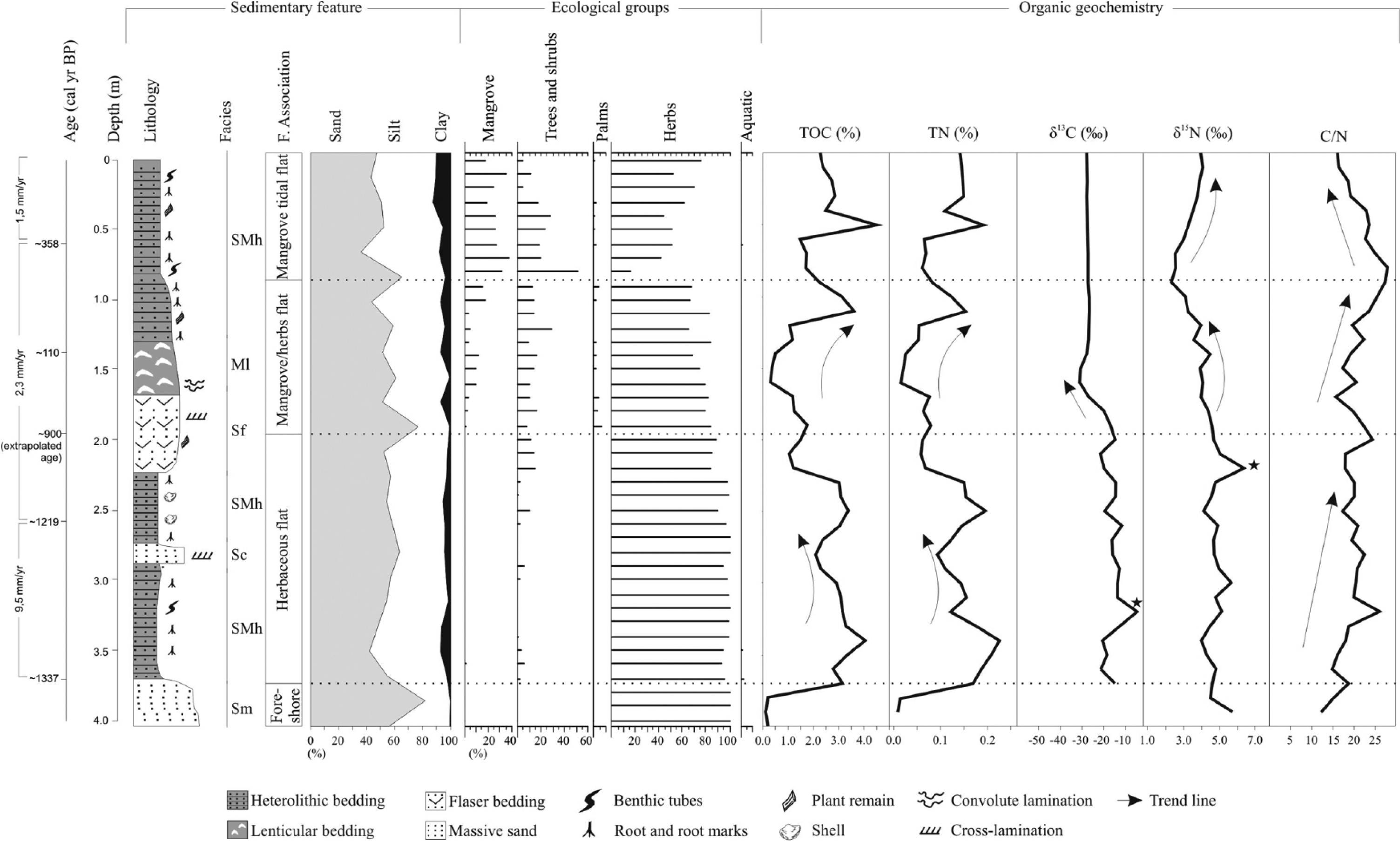
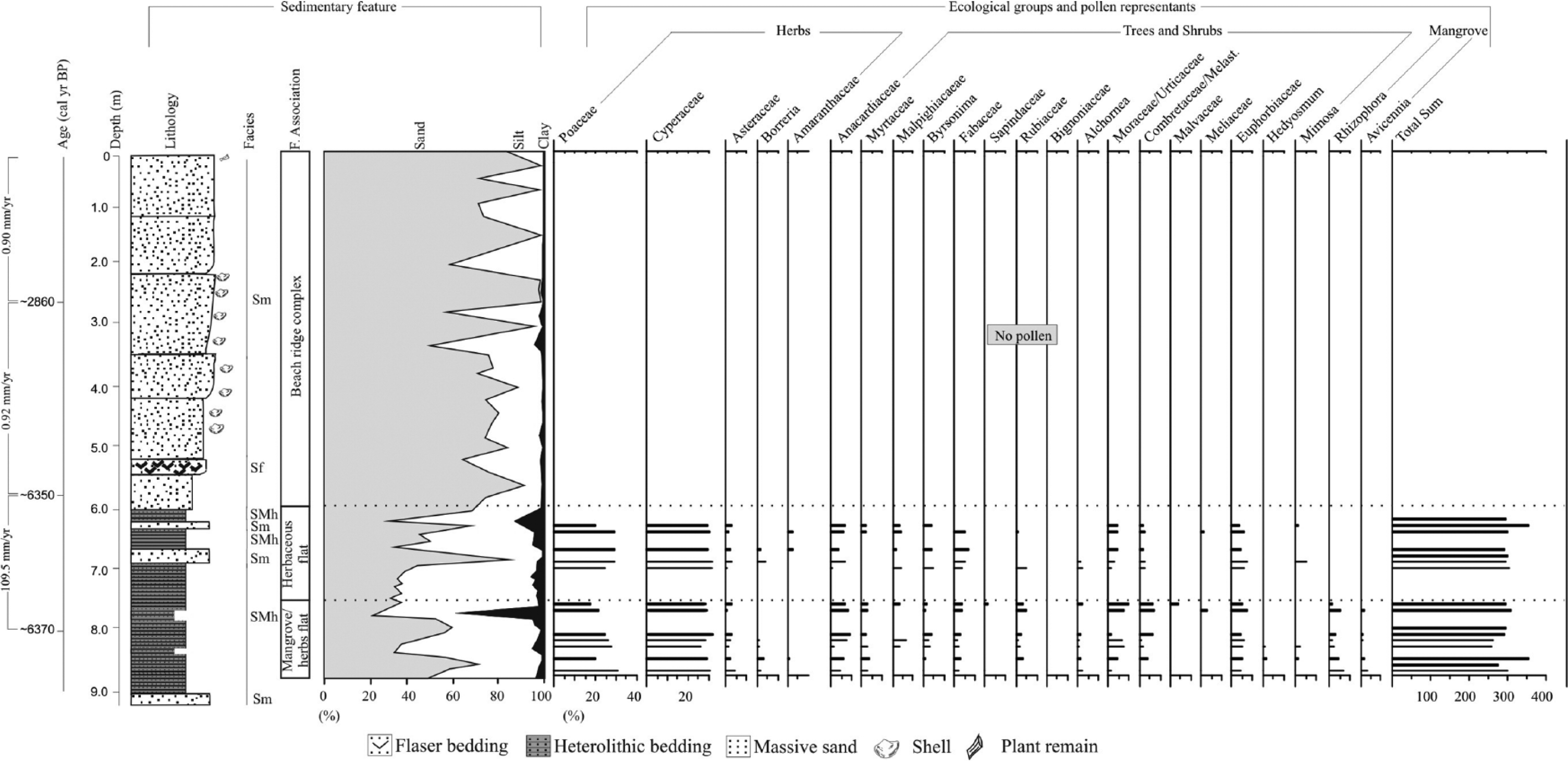
Summarized results for core LI-34, with variation as a function of core depth showing chronological and lithological profiles with sedimentary facies, as well as ecological pollen groups and geochemical variables. Pollen data are presented in the pollen diagrams as percentages of the total pollen sum.

Figure 4.

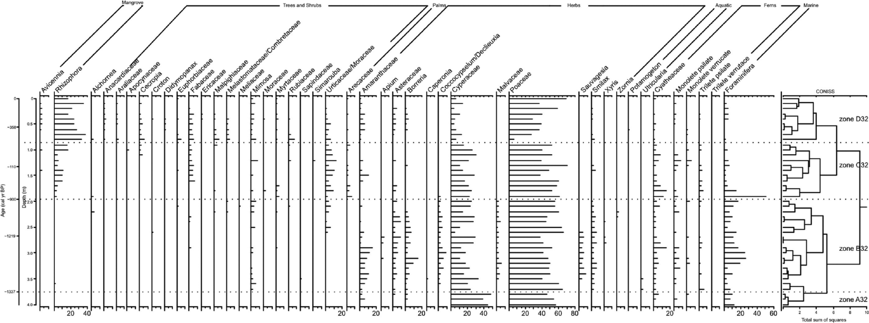
Pollen diagram record for core LI-34, with percentages of the most frequent pollen taxa, samples age, zones, and cluster analysis.

This pollen zone is marked by the dominance of herbs pollen mainly represented by Poaceae (45–55%), followed by Cyperaceae (40–50%), Amaranthaceae (3–5%), Asteraceae, and Borreria (~3%). The δ¹³C values varied from ~−32‰ to ~−28‰, and the δ¹⁵N results were between 4.4‰ and 5.7‰. The TOC results are relatively low (0.1–0.2%) at the bottom of the core, similar to the TN (~0.01%). The C/N results were between 12 and 15 (Figure 3 and Table 2).

Facies association B (herbaceous flat)

This zone is marked by the dominance of herbs pollen mainly represented by Poaceae (45–55%), followed by Cyperaceae (40–50%), Amaranthaceae (3–5%), Asteraceae, and Borreria (~3%). The δ¹³C values varied from ~−32‰ to ~−28‰, and the δ¹⁵N results were between 4.4‰ and 5.7‰. The TOC results are relatively low (0.1–0.2%) at the bottom of the core, similar to the TN (~0.01%). The C/N results were between 12 and 15 (Figure 3 and Table 2).

This facies association corresponds to the depth interval of 7.3–5.8 m in core I-3, which accumulated around 6350 cal. yr BP (Figure 5). Additionally, this facies association was observed in core LI-34 (3.7–1.9 m depth), between 1337 and ~900 cal. yr BP (Figure 3). It is characterized by mud with fine- and very fine-grained sands interbedded (facies SMb), massive sands (facies Sm), and flaser bedding (facies Sf). Cross-laminated sands (facies Sc) were observed near 2.7 m depth in core LI-34 (Figure 3). Additionally, this facies association also consists of nondetermined benthic burrows, shell fragments, roots, and root marks.

Figure 5.

Summarizing results for core I-3, with variation as a function of core depth showing chronological and lithological profiles with sedimentary facies and ecological pollen groups. Pollen data are presented in pollen diagrams as percentages of the total pollen sum.

The pollen assembly is characterized by three ecological groups (Figures 3 –5), defined by the high presence of herbs such as Poaceae (20–65%), Cyperaceae (5–35%), Amaranthaceae (3–15%), Borreria (2–15%), Asteraceae (2–10%), Sauvagesia (4–8%), Coccocyoselum or Declieuxia (2–8%), Smilax (2–7%), and Malvaceae (2–6%), followed by a low percentage (<4%) of Apium, Caperonia, Xyris, and Zornia. In this facies association, tree and shrubs were also recorded, being represented by Anacardiaceae (2–10%), Fabaceae (4–7%), Euphorbiaceae (4–7%), Mimosa (2–7%), Urticaceae or Moraceae (2–7%), Alchornea (~5%), and Byrsonima (~5%), followed by a low percentage (<4%) of Croton, Malpighiaceae, Melastomataceae or Combretaceae, Meliaceae, Myrtaceae, Rubiaceae, and Sapindaceae. Additionally, aquatic pollen was identified, characterized by Utricularia (2–3%).

The δ¹³C in core LI-34 exhibits values between −21‰ and −4.5‰ (mean = −15‰), with highest value close to 3.2 m depth (Figure 3). The δ¹⁵N record oscillates between 3.9‰ and 6.3‰ (mean = 4.7‰). The TOC and N values oscillate between 1% and 4% (mean = 2.7%) and 0.06–0.23% (mean = 0.14%), respectively. The C/N values showed an increasing trend, with variation between 14.8 and 24.3 (mean = 19.6).

Facies association C (mangrove or herbaceous flat)

Facies association C was identified in core I-3 from 9 to 7.3 m depth (~6400 cal. yr BP) and LI-34 from 1.9 to 0.9 m depth (between ~900 and ~400 cal. yr BP). The grain size is characterized by an increase of clay at the top with flaser bedding (facies Sb), lenticular bedding (facies Mb), and heterolithic bedding (facies SMb). In addition, this facies association shows cross-laminated (~1.8 m depth in LI-34) sand (facies Sc), convolute laminated sand (~1.6 m depth in LI-34). Plant remains, burrows of benthic organisms, root, and root marks are locally present (Figure 3).

The pollen record is marked by mangrove elements (Figures 3 –5), mainly consisting of Rhizophora (4–17%) and Avicennia (2–3%) pollen. Herbs are mainly represented by Poaceae (40–75%), Cyperaceae (15–30%), Amaranthaceae (5–10%), Asteraceae (3–5%), Smilax (2–5%), and Borreria (~3%). The tree and shrubs are represented by Urticaceae or Moraceae (5–15%), Anacardiaceae (2–10%), Mimosa (2–9%), Euphorbiaceae (4–8%), Melastomataceae or Combretaceae (2–7%), Fabaceae (3–5%), Byrsonima (2–5%), Myrtaceae (2–4%), and Cecropia (2–3%), followed by <5% of Alchornea, Apocynaceae, Hedyosmum, Malpighiaceae, Malvaceae, Meliaceae, Moraceae, Rubiaceae, Sapindaceae, and Simarouba. Palm pollen was also recorded (3–6%).

The isotope and elemental data in core LI-34 show different results relative to the herbaceous flat facies association (Figure 3). The δ¹³C results exhibit values between −16.8‰ and −31‰ (mean = −26.1‰). The δ¹⁵N values show an upward increased trend from 2.3‰ to 4.5‰ (mean = 3.7‰). The TOC (0.3–3.6%, mean = 1.5%), TN (0.02–0.1%, mean = 0.07%), and C/N (15.6–27.3, mean = 21.1) also show upward increased trends.

Facies association D (mangrove tidal flat)

This facies association, well represented in core LI-34, consists of heterolithic bedding (facies SMb) with roots, root marks, and plant remains, as well as undetermined dwelling burrows.

Five ecological groups (Figures 3 and 4) compose the pollen assemblage. The grains of mangrove pollen are mainly represented by Rhizophora (15–40%) and Avicennia (2–5%). Pollen of herbs are represented by Poaceae (5–65%), Cyperaceae (5–12%), Amaranthaceae (2–6%), Asteraceae (2–5%), Borreria (2–4%), and Smilax (2–4%). The tree and shrubs are characterized by low percentages (<5%) of Alchornea, Anacardiaceae, Araliaceae, Arecaceae, Cecropia, Croton, Didymopanax, Euphorbiaceae, Fabaceae, Ericaceae, Malpighiaceae, Melastomataceae or Combretaceae, Mimosa, Moraceae, Myrtaceae, Rubiaceae, and Urticaceae or Moraceae. Additionally, palm (<2%) and aquatic (<2%) pollen occur at very low percentages.

The δ¹³C values were constant (~−27‰), while the δ¹⁵N values increase upward from 2.5‰ to 4.0‰ (mean = 3.3‰). The TOC values were between 1.4% and 4.5% (mean = 2.4%) and the TN values between 0.06% and 0.19% (mean = 0.12%). The C/N values show an upward decreased trend from 27.8 to 16 (mean = 21.3).

Facies association E (beach ridge)

This facies association occurs between 5.8 and 0 m depth in core I-3 (Figure 5) and between 4.6 and 0 m depth in core I-2, being deposited during the last 6350 and ~1800 cal. yr BP, respectively (Figure 2). Core I-4 represents the most recent beach ridge phase (Figure 2 – 4.8 m depth up to the surface), as it was sampled from a beach ridge at the current coastline. These deposits are characterized by silty to fine-grained sands and laminated muds with plant remains. These lithologies grade upward into coarse-grained sands, characterizing coarsening-upward successions (Figure 2).

Facies association E displayed low pollen concentration, which is probably due to its sandier nature relative to the other facies associations. Additionally, δ¹³C, δ¹⁵N, TOC, and N were not obtained for this association.

Facies association F (tidal flat or channel)

This facies association occurs between 7.5 and 4.7 m depth in core I-2, being deposited between ~5400 and ~2040 cal. yr BP (Figure 2). It is characterized by fine- to medium-grained, parallel-laminated mud or sand and lens of massive sand (Sm). These facies are organized into fining-upward successions, and they may form packages that are erosionally based. These deposits display low pollen concentration, which is also related to its sandy lithology. δ¹³C, δ¹⁵N, TOC, and N were not obtained for this association.

Interpretation and discussion

The integration of geomorphological features, sedimentary facies, pollen data, geochemical records, and radiocarbon dates allows reconstruction of the depositional environments of the study site for the last ~6500 cal. yr BP, especially over the past ~1337 cal. yr BP. Four phases of wetland development is proposed as a result of mainly RSL changes.

Phase 1 (middle and late-Holocene)

This phase, characterized in core I-3, is represented by tidal flats occupied by mangrove forest and herbaceous vegetation in a more internal position of the coastal plain (Figures 1 and 5). During the last 6350 cal. yr BP, sands prograded over muds. Similar transition occurred at ~1800 cal. yr BP in core I-2, which is located between cores I-3 and LI-34 (Figures 2 and 6).

Figure 6.

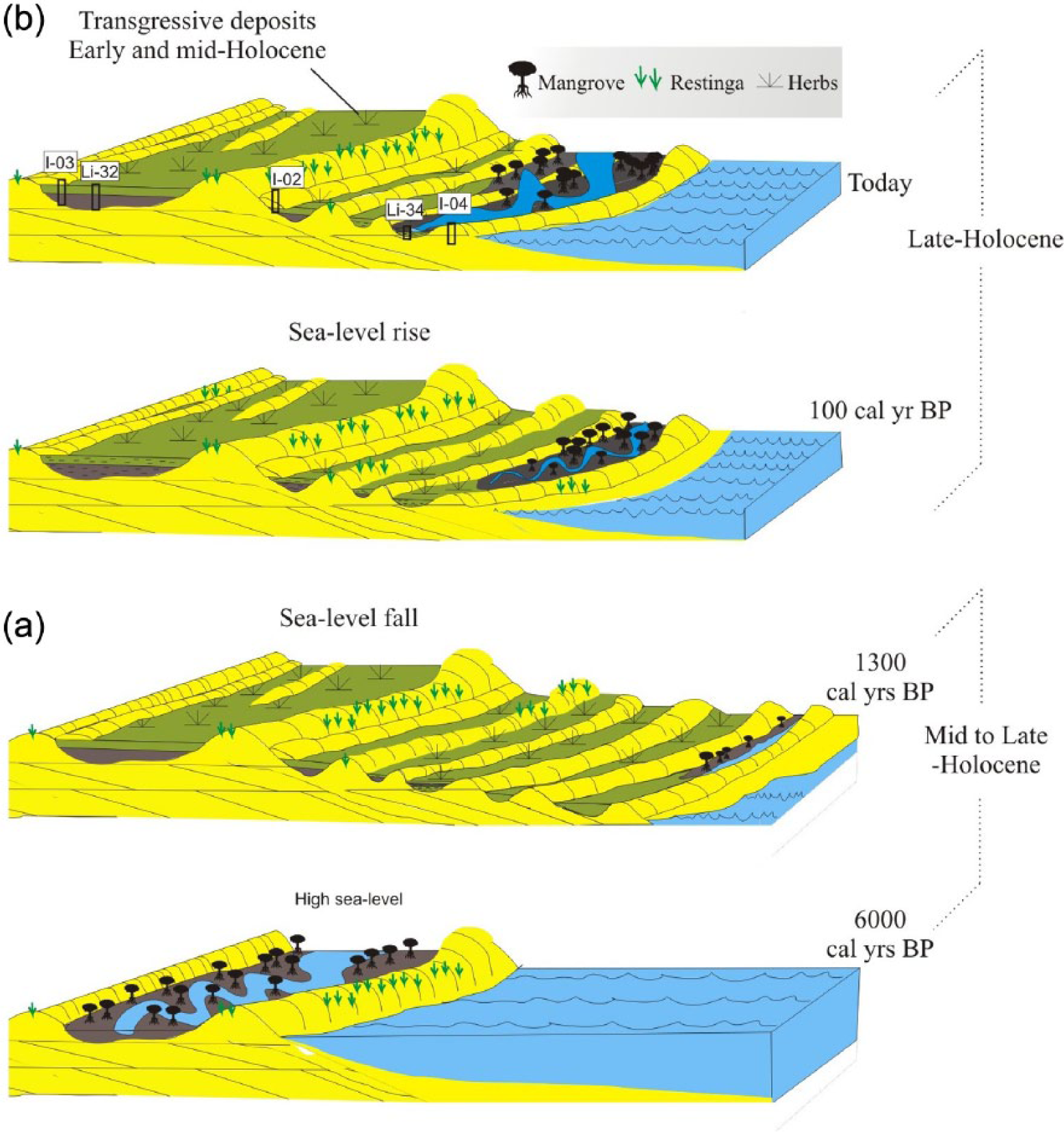
Model of the geormorphological and vegetation changes during the Holocene according to sediment supply and RSL changes: (a) first stage of progradation, with development of herbaceous flat followed by mangrove colonization (mid-Holocene to late-Holocene), and (b) second stage of progradation, with floodplain mud colonized by mangrove (late-Holocene to the present).

Phase 2 (~1337–~900 cal. yr BP)

The phase 2 was recorded in core LI-34. An herbaceous flat in the more distal portion of the studied coastal plain characterizes this phase since at least ~1337 cal. yr BP. The heterolithic bedding and the sandy layer suggest alternation of flow energy (Figure 3).

The combination of pollen data (Figure 3) and the binary diagram of δ¹³C versus C/N revealed the contribution of C₄ plants (mean = −15.5‰) and marine aquatic organic matters (Figure 7). The δ¹⁵N values (mean = 4.8‰) suggest an influence of aquatic and terrestrial organic matter (~5.0‰, Sukigara and Saino, 2005).

Figure 7.

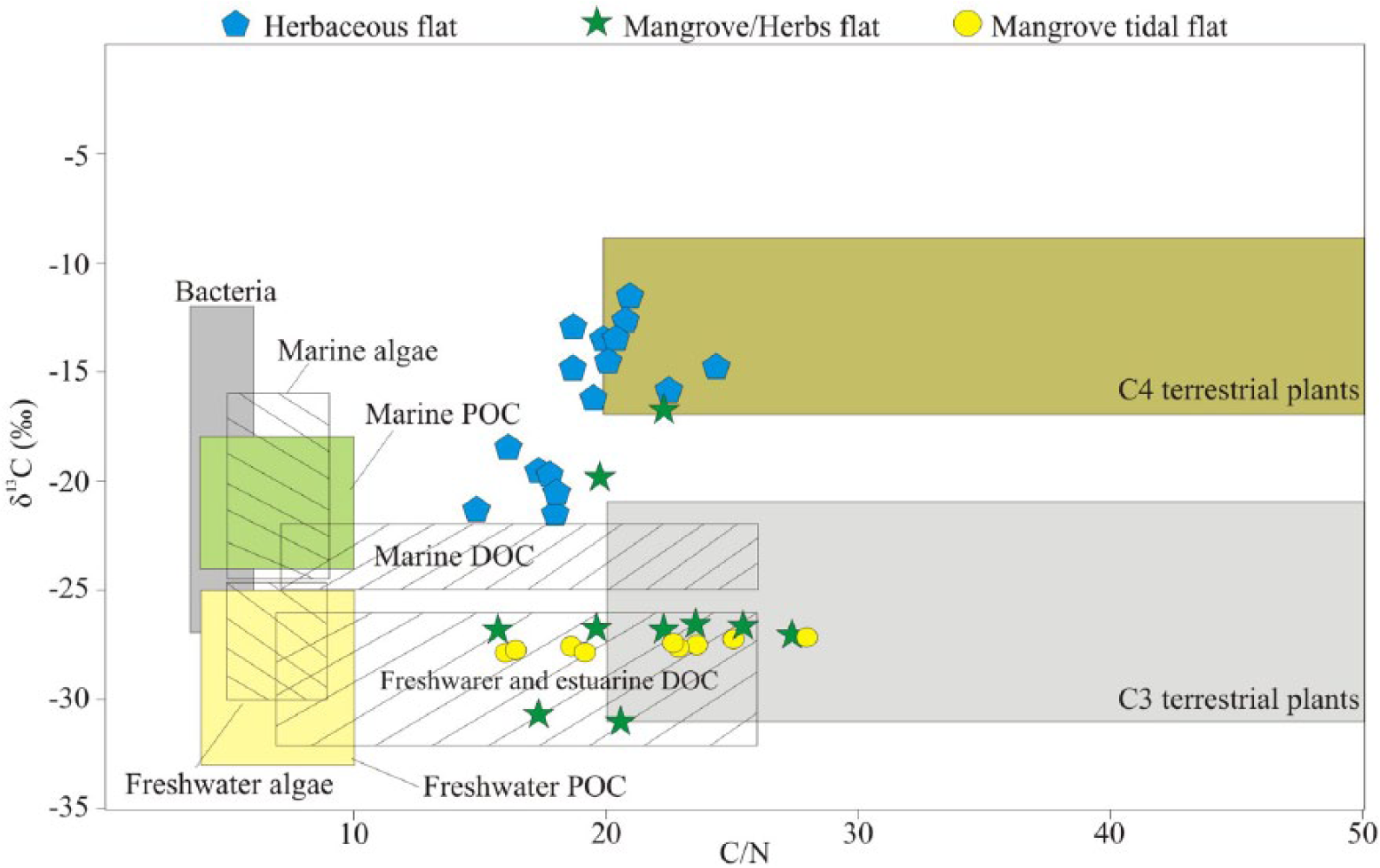
Diagram illustrating the relationship between δ¹³C and C/N for the different sedimentary facies (herbaceous flat, mangrove or herbaceous flat and mangrove tidal flat), with interpretation according to data presented by Lamb et al. (2006), Meyers (2003), and Wilson et al. (2005). C₄ plants with marine water influence and C₃ plants with freshwater and estuarine influence.

Phase 3 (~900–~400 cal. yr BP)

This phase recorded a transition between an herbaceous flat and a mangrove tidal flat. The abundance of flaser and lenticular bedding and cross-laminated sands in these environments indicates frequent alternations of flow energy (Reineck and Singh, 1980). The occurrence of convolute laminations within sandier layers of heterolithic beddings (Figure 3, 1.7–1.5 m) is related to differential forces acting on a hydroplastic sediment layer, typical of mudflats (Collinson et al., 2006). The heterolithic bedding (1.3–0.8 m) is also compatible with alternating flow energy, and the plant remains, root, and root marks indicate an abundance of plant debris. Pollen data reveal the dominance of herbs, trees, and shrubs followed by mangroves Rhizophora and Avicennia.

The upward decreased δ¹⁵N trend from 4.5‰ to 2.3‰ (core LI-34, Figure 3, 1.9–0.9 m depth) suggests an increased influence of terrestrial organic matter (Fellerhoff et al., 2003; Peterson and Howarth, 1987). Aquatic plants generally take up dissolved inorganic nitrogen, which is isotopically enriched in ¹⁵N by 7–10‰ relative to the atmospheric N (0‰). Thus, terrestrial plants that use N₂ derived from the atmosphere have δ¹⁵N values ranging from 0‰ to 2‰ (Meyers, 2003). The C/N results (mean = 21) also indicate a similar trend, with an increase in organic matter influence from vascular and terrestrial plants (>20 vascular plants, Meyers, 1994; Tyson, 1995). The binary diagram of δ¹³C versus C/N reveals the contribution of C₃ plants (Figure 7) and estuarine organic matter.

Phase 4 (~400–100 cal. yr BP to the present)

This phase is marked by mangrove development (15–40%), being characterized by Rhizophora (15–40%) and Avicennia (2–5%). The other ecological groups represented by herbs (15–75%), trees and shrubs (5–50%), and palms (<5%) may occur in association with mangrove environments. The prevalence of heterolithic bedding with abundant burrows is typical of mangrove habitats (Figure 3).

The increased values from 1.4% to 4.5% and from 0.06% to 0.19% of the TOC and TN, respectively, may be attributed to the mangrove development in the study site. The increased trend of δ¹⁵N values from 2.5‰ to 4.0‰ (mean = 3.3‰) and the decreased trend of C/N values from 27 to 16 indicate an increased influence of aquatic organic matter. In addition, the binary diagram of δ¹³C versus C/N shows an increased contribution from C₃ plants to estuarine organic matter (Figure 7). These trends might be related to an RSL rise during the last 400 cal. yr BP.

Climatic and sea-level changes affecting wetland dynamics

Regarding the studied coastal plain, the post-glacial sea-level rise caused a marine incursion with erosion of beach ridges and invasion into embayments and broad valleys. It also favored the evolution of lagoons and estuaries with wide tidal mudflats occupied by mangroves during the early Holocene and mid-Holocene, as recorded in cores I-3 (Figures 2 and 5) and LI-32 (Figure 2; França et al., 2013).

However, coastal stratigraphy and vegetation dynamics depend on the combined action of RSL oscillations and fluvial water or sedimentary supply, the latter influenced by rainfall on the drainage basin (Buso Junior, 2010; Cohen et al., 2005a, 2005b, 2012, 2014; França et al., 2013; Guimarães et al., 2012; Smith et al., 2012). This interaction affects the relative position of shorelines (Cohen et al., 2014; França et al., 2013).

Considering the Holocene climate changes, relatively drier and wetter conditions have been reported in central, southeastern, and southern Brazil during the early Holocene and mid-Holocene or late-Holocene, respectively (Barberi et al., 2000; Behling et al., 1998a, 1998b; Behling and Lichte, 1997; Ledru et al., 1996, 1998, 2009; Lorscheitter and Mattoso, 1995; Pessenda et al., 2004, 2009; Salgado-Labouriau et al., 1998; Stevaux, 1994, 2000). Variations in fluvial discharge may be a consequence of changes in rainfall rates (Amarasekera et al., 1997). Thus, a higher rainfall during the mid-Holocene and late-Holocene may have caused an increase in fluvial discharges and sediment input to coastal system (Praskievicz, 2015).

In this context, the high river sand supply and the RSL fall during the late-Holocene (Angulo et al., 2006) led to seaward and downward translation of the shoreline, producing progradational deposits and formation of extensive beach ridges over transgressive mud. During this time, the mangrove areas shrank and marshes, occupied by herbs, expanded (França et al., 2015). However, the slightly undulating relief and laterally continuous mounds of the beach ridges allowed the formation of narrow and small lagoons with mangroves at their margins, where muddy deposits were accumulated (Figure 6).

Relationship between beach ridges and mangroves

One possibility for beach ridge formation is the emergence and stabilization of sandy banks in the lower portions of beach or surf zones probably due to the submergence of coastal plain beach–dune complexes (Swift, 1975; Walker and James, 1992). Under such circumstances, the formation of lagoons and bays protected from wave and current action is favored, where occurs mud accumulation and favorable conditions for mangrove establishment. As shoreline progradation takes place, depressions between beach ridges are gradually filled until the marine inflow is cut off. This process prevents mangrove development and causes its replacement by freshwater wetlands. However, a new mangrove fringe may be established again in a lower position, where other beach ridges emerge. This mechanism has allowed the development of mangroves along the inner margins of beach ridges during a restricted time interval of decades or centuries, depending on RSL fall. Then, certain beach ridges surrounded by mangrove deposits may be used as indicators of sea levels and ancient shoreline positions (Mason, 1990; Otvos, 2000).

In contrast, RSL rise modifies delta plain through erosion of beach ridges. Such process promotes expansion of estuaries, lagoons, tidal channels, and tidal flats. The establishment and development of these environments favor mud accumulation along the estuarine salinity gradient suitable for mangrove expansion over transgressive deposits (Cohen et al., 2012; Lara and Cohen, 2006; Figure 6). In the instance of the study area, significant losses of herbaceous vegetation coverage may have occurred due to the mangrove migration into elevated areas. At this place, there is a transition between herbaceous vegetation and mangrove forest (Figures 6 and 8). The vegetation distribution on the study site follows well-known patterns, including close links between plant assemblages and topographically defined habitats (Baltzer, 1970), where salinity excludes competing, intolerant species (Snedaker, 1978). The porewater salinity is basically controlled by flooding frequency, leading to characteristic patterns of species zonation (Cohen and Lara, 2003; Lara and Cohen, 2006).

Figure 8.

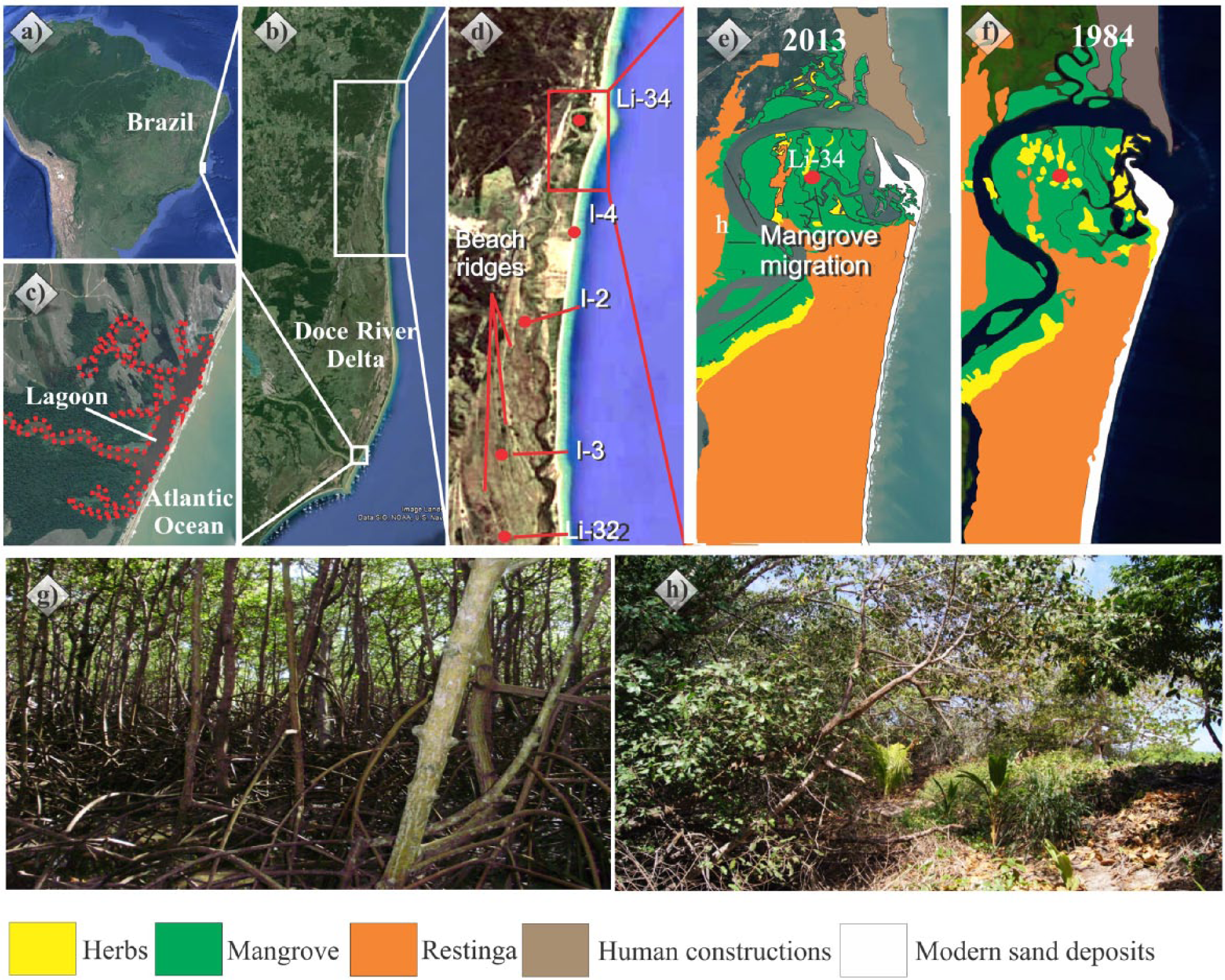
(a and b) Location of Doce River delta, (c) lake near the mouth of the Doce River, (d) localization of core LI-34, (e and f) decadal changes in mangrove area, (g) mangrove vegetation, and (h) contact between mangrove and restinga or herbaceous vegetation.

Mangrove dynamics over the last millennium

Between ~1337 and ~900 cal. yr BP (Figure 3), C₄ plants (herbs) dominated the lagoon’s margins that were flanked by beach ridges, being protected from currents, wave, and tidal action. Such environmental context would have favored mud accumulation and the inflow of terrestrial and aquatic organic matter (Figure 7). However, between ~900 and ~400 cal. yr BP, mangroves (C₃ plants) began to develop on tidal flats with increased terrestrial influence (Figure 3 – core LI-34). During the last centuries (Figure 6), the mangroves probably expanded under an increased estuarine influence, as recorded by the relation of C/N and δ¹³C values (Figure 7).

Mangrove development in the study area seems to depend on the interaction between the rates of RSL rise and sediment supply to this coastal system and the action of waves and currents. Thus, the transition from herbaceous tidal flat to mangrove, documented in core LI-34 (Figure 3), may be attributed to the adjustment of the new limits of the RSL on topographically higher terrains previously occupied by herbaceous vegetation (Figure 6).

According to pollen, isotopic and geochemical data from core LI-34 and the radiocarbon date of sample 0.6–0.64 m depth (Table 1), the study site may have been affected by an RSL rise during the last ~400 cal. yr BP. Additionally, the radiocarbon date obtained at 1.35 m depth in this same core records the beginning of mangrove establishment, indicating the possibility of an RSL rise during the last century. The age inversions detected in this core are probably related to sediment reworking due to bioturbation (Boulet et al., 1995; Gouveia and Pessenda, 2000; Pessenda et al., 2012). In addition, such inversions could also be related to the small mass and low carbon content (<0.5%) of the collected sample (LACUFF13022). Small samples can contain high amounts of young or old contaminants derived from shallow or bottom soil horizons, which may remain in the sample even after physical and chemical pretreatments. These analytical procedures remove only the adsorbed contaminants, whereas the absorbed ones can remain preserved in the residual organic matter (Pessenda et al., 2012).

Considering the possibility that the RSL rise started about 400 cal. yr BP, such event would precede the global sea-level rise recorded in the last century. However, if this rise has begun in the last century, it could be associated with the global trend that presented a rise of about 1.7 mm yr⁻¹ during the last century, with a notable increase of up to 3 mm yr⁻¹ during the last decade of the 20th century (Bindoff et al., 2007). Considering these rates of sea-level rise, expansion of lagoons and erosion of beach ridges are expected for the next decades (Figures 6 and 8), and terrains occupied by freshwater swamps, positioned on higher elevations, will be re-colonized by mangroves due to increased marine influence (Cohen and Lara, 2003; Soares, 2009).

Mangrove changes during the last decades

The time series analysis of satellite images for a 29 years interval indicates important geomorphologic and vegetation changes (Figure 8). The lagoon, where the studied mangroves are located, truncates beach ridges, and the mangroves are migrating to topographic higher position occupied by herbaceous vegetation. For instance, the sampling site represented by core LI-34 exhibits a tidal flat colonized by mangroves. However, according to the satellite image obtained from 1984, this site was occupied by herbaceous vegetation (Figure 8), as indicated by pollen analyses (Figures 3 and 4). A similar situation was described in the northern Brazilian littoral (Cohen and Lara, 2003; França et al., 2012).

This landward mangrove migration during the last decades and the erosion of beach ridges by lagoons may be related to a modern sea-level rise frequently referred in the literature (e.g. Bindoff et al., 2007). The topography-dependent mangrove dynamics strongly suggests an increase in inundation frequency, changes in soil salinity, and transportation of mangrove seeds into more elevated areas (Cohen and Lara, 2003; Lara and Cohen, 2006).

Other causes for lagoon expansion and mangrove migration in the studied site may be proposed. For instance, changes in fluvial discharge and rainfall oscillations could have affected both water salinity and water level. These changes could have been cyclical along the coast, because of littoral currents, which may have obstructed the connection of the lagoon with the sea. For instance, a modern lake near the Doce River’s mouth (Figure 8c) is not connected with seawaters. Consequently, the dominant vegetation on the edge of this lagoon is freshwater wetland. However, if the connection between the lagoon and the sea returns, the mangrove will expand on this area. Then, the drift currents transporting sediments along the coastline may cause recurrent episodes of disconnection between the lagoon and the sea, affecting a local vegetation succession within a determined time scale (in this case, decades).

In this context, the driving forces behind the vegetation changes in the study area could be explained by the autocyclic and allocyclic processes (Busch and Rollins, 1984). Autocyclic processes are intrabasinal in origin, and are related to sedimentary dynamics. Autocycles may be caused by tides and storms, and they show limited stratigraphic continuity. In deltaic systems, such processes may include lobe switching, river avulsion, meandering, and fluvial point-bar migration or lateral migration of beach-barrier bars. Allocyclic processes are extrabasinal in origin and can include for instance climate changes, sea-level fluctuations and tectonics. These processes tend to produce more widespread impacts on the sedimentary record (Walker and James, 1992).

Thus, vegetation changes during the Holocene in the study site are more likely associated with allocyclic processes because important changes in facies associations occurred, which are consistent with RSL fluctuations and with the climatic changes recorded along the southeastern coast of Brazil. However, the mangrove migration recorded by satellite images during the last decades, with transition from herbaceous tidal flats into mangroves and the terrestrial to estuarine organic matter revealed by pollen and biogeochemical data during the last century(ies), may be related to a long-term trend controlled by a tendency of RSL rise (allocyclic process) and/or sediment transport along the coastline (autocyclic process).

Conclusion

Our data show the response of coastal wetlands to changes in RSL and fluvial discharge during the mid-Holocene and late-Holocene. During the mid-Holocene, tidal flats positioned on topographically high terrains along the edge of a lagoon sheltered by beach ridges were occupied by wetlands represented by mangrove trees and herbs. During the last ~6350 cal. yr BP, the RSL fall and the higher discharge of fluvial sediment would have promoted coastal progradation. These processes would have also led to the formation of extensive beach ridges over transgressive mud deposits. The latter accumulated in lagoons and tidal flats and led to mangrove shrinking. A similar transition was recorded in a relatively lower and more distal position at ~3043 cal. yr BP.

Between ~1337 and ~900 cal. yr BP, a tidal flat on the edge of a lagoon was colonized by herbaceous (C₄ plants) vegetation and accumulated marine organic matter. However, the contribution of terrestrial organic matter increased through time. The next phase, between ~900 and ~400 or ~100 cal. yr BP, is marked by the transition between herbaceous tidal flat and mangrove, as indicated by the increased inflow of terrestrial organic matter. During the past ~400 or ~100 cal. yr BP, mangrove vegetation became stable as indicated by pollen analysis, followed by an increased contribution of estuarine organic matter.

The last phase of mangrove establishment and the increased contribution of estuarine organic matter recorded in the last centuries may be associated with an RSL rise. Under this condition, erosion of beach ridges and expansion of lagoons and mangroves as recorded in the time series analyses are expected. However, considering the several forces that may influence mangrove dynamics, further detailed studies consisting of the monitoring of mangrove forests by satellite images, added to fieldwork, are still needed in order to identify the influence of RSL rise on the distribution of mangroves along the littoral of the State of Espírito Santo, Southeastern Brazil.

Footnotes

Acknowledgements

We would like to thank the members of the Laboratory of Coastal Dynamics (LADIC-UFPA), ¹⁴C Laboratory of Center for Nuclear Energy in Agriculture (CENA-USP), Vale Natural Reserve (Linhares, ES), and the students from the Laboratory of Chemical-Oceanography (UFPA).

Funding

This study was supported by FAPESP (03615-5/2007 and 00995-7/11) and National Institute on Science and Technology in Tropical Marine Environments – INCT-AmbTropic (CNPq Process 565054/2010-4).

References

Absy

(1975) Polen e esporos do Quaternário de Santos (Brasil). Hoehnea 5: 1–26.

Alongi

(2008) Mangrove forests: Resilience, protection from tsunamis, and responses to global climate change. Estuarine, Coastal and Shelf Science 76: 1–13.

Alongi

(2012) Carbon sequestration in mangrove forests. Carbon Management 3: 313–322.

Alongi

(2014) Carbon cycling and storage in mangrove forests. Annual Review of Marine Science 6: 195–219.

Amarasekera

Lee

Williams

. et al. (1997) ENSO and the natural variability in the flow of tropical rivers. Journal of Hydrology 200: 24–39.

Angulo

Lessa

Souza

(2006) A critical review of mid- to late-Holocene sea-level fluctuations on the eastern Brazilian coastline. Quaternary Science Reviews 25: 486–506.

Arai

(2006) A grande elevação eustática do Mioceno e sua influência na origem do Grupo Barreiras. Geologia USP: Série Científica 6: 1–6.

Asmus

Gomes

Pereira

ACB

(1971) Integração geológica regional da bacia do Espírito Santo. In: Anais do XXV Congresso Brasileiro de Geologia (SBG), São Paulo, September 1971, pp. 235–254.

Baltzer

(1970) Etude sédimentologique du marais de Mara (Côte ouest de la Nouvelle Calédonie) et de formations quaternaires voisines. Mémoires expédition française sur lês récifs coralliens de la Nouvelle Calédonie. Foundation Singer-Polignac 4: 146–169.

10.

Barberi

Salgado-Labouriau

Suguio

(2000) Paleovegetation and Paleoclimate of ‘Vereda de Águas Emendadas’, central Brazil. Journal of South American Earth Sciences 13: 241–254.

11.

Behling

Lichte

(1997) Evidence of dry and cold climatic conditions at glacial times in tropical Southeastern Brazil. Quaternary Research 48: 348–358.

12.

Behling

Hooghiemstra

Bonnefille

(1998a) Intertropical Last Glacial and Holocene climatic change (Preface). Review of Palaeobotany and Palynology 99: 75–76.

13.

Behling

Hooghiemstra

Negret

(1998b) Holocene history of the Choco rain forest from Laguna Piusbi, southern Pacific lowlands of Colombia. Quaternary Research 50: 300–308.

14.

Bernini

Silva

MAB

Carmo

TMS

. et al. (2006) Composição química do sedimento e de folhas das espécies do manguezal do estuário do Rio São Mateus, Espírito Santo, Brasil. Revista Brasileira de Botânica 29: 689–699.

15.

Bindoff

Willebrand

Artale

. et al. (2007) Observations: Oceanic climate change and sea level. In: Solomon

Qin

Manning

. et al. (eds) Climate Change 2007: The Physical Science Basis – Contribution of Working Group I to the Fourth Assessment Report of the Intergovernmental Panel on Climate Change. Cambridge: Cambridge University Press, pp. 385–431.

16.

Blasco

Saenger

Janodet

(1996) Mangrove as indicators of coastal change. Catena 27: 167–178.

17.

Boulet

Pessenda

LCR

Telles

ECC

(1995) Une évaluation de la vitesse de l’accumulation superficielle de matière par la faune du sol à partir de la datation des charbons et de l’humine du sol. Exemple des latosols des versants du lac Campestre, Salitre, Minas Gerais, Brésil. Comptes Rendus de L’académie Des Sciences 320: 287–294.

18.

Busch

Rollins

(1984) Correlation of Carboniferous strata using a hierarchy of transgressive-regressive units. Geology 12: 471.

19.

Buso Junior

(2010) Dinâmica ambiental holocênica (vegetação, clima e nível relativo marinho) baseada em estudos interdisciplinares de alta resolução, no litoral norte do estado do Espírito Santo. Master Thesis, Universidade de São Paulo.

20.

Buso Junior

Pessenda

Oliveira

. et al. (2013) From an estuary to a freshwater lake: A paleo-estuary evolution in the context of Holocene sea-level fluctuations, southeastern Brazil. Radiocarbon 55: 1735–1746.

21.

Camargo

(1999) Software para análise granulométrica SysGran, versão 3.0. Curitiba: UFPR.

22.

Carvalho

LMV

Jones

Liebmann

(2004) The South Atlantic convergence zone: Intensity, form, persistence, and relationships with intraseasonal to interannual activity and extreme rainfall. Journal of Climate 17: 88–108.

23.

Castro

Rossetti

Cohen

MCL

. et al. (2013) The growth of the Doce River Delta in northeastern Brazil indicated by sedimentary facies and diatoms. Diatom Research 28: 455–466.

24.

Church

Clark

Cazenave

. et al. (2013) Sea level change. In: Stocker

Qin

Plattner

G-K

. et al. (eds) Climate Change 2013: The Physical Science Basis. Cambridge; New York: Cambridge University Press, pp. 1137–1216.

25.

Cohen

MCL

(2003) Past and current mangrove dynamics on the Bragança península, northern Brasil. PhD Thesis, Universität Bremen.

26.

Cohen

MCL

Lara

(2003) Temporal changes of mangrove vegetation boundaries in Amazonia: Application of GIS and remote sensing techniques. Wetlands Ecology and Management 11: 223–231.

27.

Cohen

MCL

Behling

Lara

(2005a) Amazonian mangrove dynamics during the last millennium: The relative sea-level and the Little Ice Age. Review of Palaeobotany and Palynology 136: 93–108.

28.

Cohen

MCL

França

Rossetti

. et al. (2014) Landscape evolution during the late Quaternary at the Doce River mouth, Espírito Santo State, Southeastern Brazil. Palaeogeography, Palaeoclimatology, Palaeoecology 415: 48–58.

29.

Cohen

MCL

Lara

Smith

. et al. (2009) Impact of sea-level and climatic changes on the Amazon coastal wetlands during the late-Holocene. Vegetation History and Archaeobotany 18: 425–439.

30.

Cohen

MCL

Pessenda

LCR

Behling

. et al. (2012) Holocene palaeoenvironmental history of the Amazonian mangrove belt. Quaternary Science Reviews 55: 50–58.

31.

Cohen

MCL

Souza Filho

Lara

. et al. (2005b) A model of Holocene mangrove development and relative sea-level changes on the Bragança Peninsula (northern Brazil). Wetlands Ecology and Management 13: 433–443.

32.

Colinvaux

De Oliveira

Patiño

JEM

(1999) Amazon Pollen Manual and Atlas. Dordrecht: Harwood Academic Publishers.

33.

Collinson

Mountney

Thompson

(2006) Sedimentary Structures. Edinburgh: Dunedin Academic Press.

34.

Deines

(1980) The isotopic composition of reduced organic carbon. In: Fritz

Fontes

(eds) Handbook of Environmental Isotope Geochemistry. Amsterdam: Elsevier, pp. 329–406.

35.

Departamento de Hidrografia e Navegação (2014) Marinha do Brasil. Rio de Janeiro: DHN.

36.

Dittmar

Hertkorn

Kattner

. et al. (2006) Mangroves, a major source of dissolved organic carbon to the oceans. Global Biogeochemical Cycles 20: 1–7.

37.

Dominguez

JML

Bittencourt

ACSP

Martin

(1992) Controls on Quaternary coastal evolution of the east-northeastern coast of Brazil: Roles of sea-level history, trade winds and climate. Sedimentary Geology 80: 213–232.

38.

Dominguez

JML

Andrade

ACS

Almeida

. et al. (2009) The Holocene barrier strandplains of the State of Bahia. In: Dillenburg

Hesp

(eds) Geology and Geomorphology of Holocene Coastal Barriers of Brazil. Berlin: Springer, pp. 253–288.

39.

Donato

Kauffman

Murdiyarso

. et al. (2011) Mangroves among the most carbon-rich forests in the tropics. Nature Geoscience 4: 293–297.

40.

Duke

Meynecke

Dittmann

. et al. (2007) A world without mangroves? Science 317: 41–42.

41.

Ewel

Twilley

Ong

(1998) Different kinds of mangrove forests provide different goods and services. Global Ecology and Biogeography Letters 7: 83–94.

42.

Faegri

Iversen

(1989) Textbook of Pollen Analysis. Chichester: Wiley.

43.

Fellerhoff

Voss

Wantzen

(2003) Stable carbon and nitrogen isotope signatures of decomposing tropical macrophytes. Aquatic Ecology 37: 361–375.

44.

França

Alves

ICC

Castro

. et al. (2015) A multi-proxy evidence for the transition from estuarine mangroves to deltaic freshwater marshes, Southeastern Brazil, due to climatic and sea-level changes during the late-Holocene. Catena 128: 155–166.

45.

França

Cohen

MCL

Pessenda

LCR

. et al. (2013) Mangrove vegetation changes on Holocene terraces of the Doce River, Southeastern Brazil. Catena 110: 59–69.

46.

França

Francisquini

Cohen

MCL

. et al. (2012) The last mangroves of Marajó Island – Eastern Amazon: Impact of climate and/or relative sea-level changes. Review of Palaeobotany and Palynology 187: 50–65.

47.

Fromard

Vega

Proisy

(2004) Half a century of dynamic coastal change affecting mangrove shorelines of French Guiana: A case study based on remote sensing data analysis and field surveys. Marine Geology 208: 265–280.

48.

Giri

Ochieng

Tieszen

. et al. (2011) Status and distribution of mangrove forests of the world using earth observation satellite data. Global Ecology and Biogeography 20: 154–159.

49.

Goh

(2006) Removal of contaminants to improve the reliability of radiocarbon dates of peats. Journal of Soil Science 29: 340–349.

50.

Gouveia

SEM

Pessenda

LCR

(2000) Datation par le C-14 de charbons inclus dans le sol pour l’étude du rôle de la remontée biologique de matière et du colluvionnement dans la formation de latosols de l’état de São Paulo, Brésil. Comptes Rendus de L’académie Des Sciences 330: 133–138.

51.

Grimm

(1987) CONISS: A FORTRAN 77 program for stratigraphically constrained cluster analysis by the method of the incremental sum of squares. Computers & Geosciences 13: 13–35.

52.

Grimm

(1990) TILIA and TILIAGRAPH: PC spreadsheet and graphic software for pollen data. INQUA Sub-Commission on Data-Handling Methods Newsletter 4: 5–7.

53.

Grinsted

Moore

Jevrejeva

(2009) Reconstructing sea level from paleo and projected temperatures 200 to 2100AD. Climate Dynamics 34: 461–472.

54.

Guimarães

JTF

Cohen

MCL

Pessenda

LCR

. et al. (2012) Mid and late-Holocene sedimentary process and palaeovegetation changes near the mouth of the Amazon River. The Holocene 22: 359–370.

55.

Harper

(1984) Improved methods of facies sequence analysis. In: Walker

James

(eds) Facies Models – Response to Sea Level Change. Ottawa: Geological Association of Canada, pp. 11–13.

56.

Lamb

Wilson

Leng

(2006) A review of coastal palaeoclimate and relative sea-level reconstructions using δ¹³C and C/N ratios in organic material. Earth-Science Reviews 75: 29–57.

57.

Lara

Cohen

MCL

(2006) Sediment porewater salinity, inundation frequency and mangrove vegetation height in Bragança, North Brazil: An ecohydrology-based empirical model. Wetlands Ecology and Management 4: 349–358.

58.

Ledru

Mourguiart

Riccomini

(2009) Related changes in biodiversity, insolation and climate in the Atlantic rainforest since the last interglacial. Palaeogeography, Palaeoclimatology, Palaeoecology 271: 140–152.

59.

Ledru

Salgado-Labouriau

Lorscheitter

(1996) The last 50,000 years in the Neotropics (Southern Brazil): Evolution of vegetation and climate. Palaeogeography, Palaeoclimatology, Palaeoecology 123: 239–257.

60.

Ledru

Salgado-Labouriau

Lorscheitter

(1998) Vegetation dynamics in southern and central Brazil during the last 10,000 yr BP. Review of Palaeobotany and Palynology 99: 131–142.

61.

Lorscheitter

Mattoso

(1995) Reconstituição paleoambiental da região dos Campos Gerais, Paraná, através da palinologia de sedimentos da Lagoa Dourada. In: V Congresso da Associação Brasileira de Estudos do Quaternário (ed ABEQUA), Niterói, 3–9 July, pp. 18–21. Niterói: Anais.

62.

McLeod

Salm

(2006) Managing Mangroves for Resilience to Climate Change. Gland: IUCN.

63.

Markgraf

D’Antoni

(1978) Pollen Flora of Argentina. Tucson, AZ: University of Arizona Press.

64.

Martin

Suguio

(1992) Variation of coastal dynamics during the last 7000 years recorded in beach-ridge plains associated with river mouths: Example from the central Brazilian coast. Palaeogeography, Palaeoclimatology, Palaeoecology 99: 119–140.

65.

Martin

Dominguez

JML

Bittencourt

ACSP

(1998) Climatic control on coastal erosion during a sea-level fall episode. Anais da Academia Brasileira de Ciências 70: 249–266.

66.

Martin

Suguio

Flexor

. et al. (1996) Quaternary sea-level history and variation in dynamics along the central Brazil Coast: Consequences on coastal plain construction. Anais da Academia Brasileira de Ciências 68: 303–354.

67.

Mason

(1990) Beach ridge geomorphology of Kotzebue Sound: Implications or paleoclimatology and archaeology. PhD Thesis, University of Alaska Fairbanks.

68.

Masselink

Gehrels

(2014) Coastal Environments and Global Change: Processes and Adaptation. Chichester: Wiley-Blackwell.

69.

Meyers

(1994) Preservation of elemental and isotopic source identification of sedimentary organic matter. Chemical Geology 114: 289–302.

70.

Meyers

(1997) Organic geochemical proxies of paleoceanographic, paleolimnologic and paleoclimatic processes. Organic Geochemistry 27: 213–250.

71.

Meyers

(2003) Applications of organic geochemistry to paleolimnological reconstructions: A summary of examples from the Laurentian Great Lakes. Organic Geochemistry 34: 261–289.

72.

Miall

(1978) Facies types and vertical profile models in braided river deposits: A summary. In: Miall

(ed.) Fluvial Sedimentology. Calgary: Canadian Society of Petroleum Geologists, pp. 597–604.

73.

Milne

Long

Bassett

(2005) Modelling Holocene relative sea-level observations from the Caribbean and South America. Quaternary Science Reviews 24: 1183–1202.

74.

Miranda

MCC

Rossetti

Pessenda

LCR

(2009) Quaternary paleoenvironments and relative sea-level changes in Marajó Island (Northern Brazil): Facies, δ¹³C, δ¹⁵N and C/N. Palaeogeography, Palaeoclimatology, Palaeoecology 282: 19–31.

75.

Munsell Color (2009) Munsell Soil Color Charts. New Revised Edition. New Windsor, NY: Macbeth Division of Kollmorgen Instruments.

76.

Otvos

(2000) Beach ridges – Definitions and significance. Geomorphology 32: 83–108.

77.

Peixoto

Gentry

(1990) Diversidade e composição florística da mata de tabuleiros na Reserva Florestal de Linhares (Espírito Santo, Brasil). Revista Brasileira de Botânica 13: 19–25.

78.

Pessenda

LCR

De Oliveira

Mofatto

. et al. (2009) The evolution of a tropical rainforest/grassland mosaic in Southeastern Brazil since 28,000 14C yr BP based on carbon isotopes and pollen records. Quaternary Research 71: 437–452.

79.

Pessenda

LCR

Gouveia

SEM

Aravena

. et al. (2004) Holocene fire and vegetation changes in Southeastern Brazil as deduced from fossil charcoal and soil carbon isotopes. Quaternary International 114: 35–43.

80.

Pessenda

LCR

Saia

SEMG

Gouveia

SEM

. et al. (2010) Last millennium environmental changes and climate inferences in the Southeastern Atlantic Forest, Brazil. Anais da Academia Brasileira de Ciências 82: 717–729.

81.

Pessenda

LCR

Vidotto

De Oliveira

. et al. (2012) Late Quaternary vegetation and coastal environmental changes at Ilha do Cardoso mangrove record, Southeastern Brazil. Palaeogeography, Palaeoclimatology, Palaeoecology 363: 57–68.

82.

Peterson

Howarth

(1987) Sulfur, carbon, and nitrogen isotopes used to trace organic matter flow in the salt-marsh estuary of Sapelo Island, Georgia. Limnology and Oceanography 32: 1195–1213.

83.

Praskievicz

(2015) A coupled hierarchical modeling approach to simulating the geomorphic response of river systems to anthropogenic climate change. Earth Surface Processes and Landforms 40: 1616–1630.

84.

Reimer

Baillie

MGL

Bard

. et al. (2009) IntCal09 and Marine09 radiocarbon age calibration curves, 0–50,000 years cal BP. Radiocarbon 51: 1111–1150.

85.

Reineck

Singh

(1980) Depositional Sedimentary Environments with Reference to Terrigenous Clastics. Berlin: Springer-Verlag.

86.

Reis

Maia

RMC

Silva

. et al. (2013) Origin of step-like and lobate seafloor features along the continental shelf off Rio de Janeiro State, Santos Basin-Brazil. Geomorphology 203(V. Special): 25–45.

87.

Rossetti

Valeriano

(2007) Evolution of the lowest Amazon basin modeled from the integration of geological and SRTM topographic data. Catena 70: 253–265.

88.

Rossetti

Góes

Valeriano

. et al. (2008) Quaternary tectonics in a passive margin: Marajó Island, northern Brazil. Journal of Quaternary Science 23: 121–135.

89.

Rossetti

Polizel

Cohen

MCL

. et al. (2015) Depositional evolution of the Doce River delta, Southeastern Brazil, in the context of sea−level and climatic changes during the Late Pleistocene-Holocene. Marine Geology 367: 171–190.

90.

Roubik

Moreno

(1991) Pollen and Spores of Barro Colorado Island. St. Louis, MO: Missouri Botanical Garden.

91.

Salgado-Labouriau

(1997) Late Quaternary palaeoclimate in the savannas of South America. Journal of Quaternary Science 12: 371–379.

92.

Salgado-Labouriau

Barberi

Ferrazvicentini

. et al. (1998) A dry climatic event during the Late Quaternary of Tropical Brazil. Review of Palaeobotany and Palynology 99: 115–129.

93.

Schaeffer-Novelli

Cintrón-Molero

Adaima

(1990) Variability of mangrove ecosystems along the Brazilian coast. Estuaries 13: 204–218.

94.

Schidlowski

Hayes

Kaplan

(1983) Isotopic inferences of ancient biochemistries: Carbon, sulphur, hydrogen and nitrogen. In: Scholf

(ed.) Earth’s Earliest Biosphere, Its Origin and Evolution. Princeton, NJ: Princeton University Press, pp. 149–186.

95.

Smith

Cohen

MCL

Pessenda

LCR

. et al. (2012) Holocenic proxies of sedimentary organic matter and the evolution of Lake Arari-Amazon Region. Catena 90: 26–38.

96.

Snedaker

(1978) Mangroves: Their value and perpetuation. Natural Resources 16: 179–188.

97.

Soares

MLG

(2009) A conceptual model for the responses of mangrove forests to sea level rise. Journal of Coastal Research 56(SI): 267–271.

98.

Stevaux

(1994) The upper Paraná river (Brazil): Geomorphology, sedimentology and paleoclimatology. Quaternary International 21: 143–161.

99.

Stevaux

(2000) Climatic events during the late Pleistocene and Holocene in the Upper Parana River: Correlation with NE Argentina and South-Central Brazil. Quaternary International 72: 73–85.

100.

Sukigara

Saino

(2005) Temporal variations of δ¹³C and δ¹⁵N in organic particles collected by a sediment trap at time-series station off the Tokyo Bay. Continental Shelf Research 25: 1749–1767.

101.

Swift

DJP

(1975) Barrier island genesis: Evidence from the central Atlantic Shelf, eastern USA. Sedimentary Geology 14: 1–43.

102.

Thornton

McManus

(1994) Applications of organic carbon and nitrogen stable isotope and C/N ratios as source indicators of organic matter provenance in estuarine systems: Evidence from the Tay Estuary, Scotland. Estuarine, Coastal and Shelf Science 38: 219–233.

103.

Tyson

(1995) Sedimentary Organic Matter: Organic Facies and Palynofacies. London: Chapman & Hall.

104.

Walker

James

(1992) Facies Models – Response to Sea Level Change. Ottawa: Geological Association of Canada.

105.

Walsh

Nittrouer

(2004) Mangrove-bank sedimentation in a mesotidal environment with large sediment supply, Gulf of Papua. Marine Geology 208: 225–248.

106.

Wentworth

(1922) A scale of grade and class terms for clastic sediments. Journal of Geology 30: 377–392.

107.

Wilson

Lamb

Leng

. et al. (2005) δ¹³C and C/N as potential coastal palaeoenvironmental indicators in the Mersey Estuary, UK. Quaternary Science Reviews 24: 2015–2029.

108.

Woodcock

Allen

Anderson

. et al. (2008) Free access to Landsat imagery. Science 320(5879): 1011.

109.

Gong

(2011) Google Earth as a virtual globe tool for Earth science applications at the global scale: Progress and perspectives. International Journal of Remote Sensing 33(12): 3966–3986.