
Abstract
Hitherto, the Landscape Reconstruction Algorithm (LRA) has been the only truly quantitative approach to stand-scale palynology. However, the LRA requires information on pollen productivity and dispersal, which is not always available. The alternative approach MARCO POLO (MAnipulating pollen sums to ReCOnstruct POllen of Local Origin) presented here is solely based on pollen values and does not rely on a pollen dispersal function. In a stepwise fashion, MARCO POLO removes those pollen types from the pollen sum whose values are significantly higher than in a neighbouring large basin. The resulting regional pollen sum is free of the disturbing factor of (extra-)local pollen. Based on this sum, comparison with the pollen record from the large basin allows calculating sharp (extra-)local signals. Treating the (extra-)local pollen portion with representation factors (R-values) then produces a quantitative reconstruction of the stand-scale vegetation composition. We tested MARCO POLO and the LRA on a dataset of pollen surface samples and forest vegetation relevés from northern Central Europe. Both approaches reconstruct the presence or absence of taxa at the stand scale within a small margin of error. Where observed cover was ⩾2%, both models always reconstructed presence, where modelled cover was ⩾2% the taxon was always present. Overall, both approaches perform well in reconstructing the cover of taxa within a 100-m radius. In our tests, MARCO POLO is slightly better at reconstructing cover values for more taxa. Although some model parameters evidently need revision, the simple correlative approach of MARCO POLO appears to perform at least as well as the complex LRA model.
Keywords
Introduction
The reconstruction of forest cover and composition has always played a central role in Holocene palaeoecology. Pollen-based quantitative reconstructions of past forest composition commonly use records from large basins focussing on vegetation development in the wider surrounding landscape. The changes on that large scale do not necessarily represent the actual changes in forest communities at the stand scale that result from processes such as competition, succession and disturbance. Actuo-ecological studies at the community level can help interpret the palaeo-record, but they typically cover time periods of a few years to several decades only. Using (sub)fossil records, palaeoecology may achieve a similarly high temporal resolution, but extend the time scale to thousands of years (or more).
Fossil pollen provides particularly abundant records of past vegetation, but pollen is transported over long distances and typically reflects (past) vegetation at much larger spatial scales than of interest to community-level ecology. Still, most of the pollen is deposited close to its source (Janssen, 1966; Tauber, 1965) and different sized basins record pollen from different sources. Whereas large lakes mainly record pollen from the wider surroundings, pollen from close by dominates in records from terrestrial soils, small ponds or peatlands and mineral soil to peat transitions (regional vs. (extra-)local pollen sensu Janssen, 1966; Jacobson and Bradshaw, 1981). Small basins, such as forest depressions, are therefore well suited to reconstruct the changes in vegetation patterns at the stand scale.
However, in small basins there is still a significant regional component to the pollen load. Hence, one challenge of so-called stand-scale palynology (Bradshaw, 2013) is to distinguish between pollen from close by and farther away (Jacobson and Bradshaw, 1981; Oldfield, 1970). Attempts have been made to identify pollen of (extra-)local origin by comparing pollen data between sites, using approaches of varying degree of complexity (Bradshaw, 1981; Heide, 1984; Jacobson, 1979; Sugita et al., 2006), but the results remained semi-quantitative only. The modern analogue approach of Davis et al. (1994, 1998) has produced convincing results, but can only reconstruct communities that have modern analogues, which is rarely the case in Central Europe. A true quantitative approach to stand-scale reconstructions has been proposed with the Landscape Reconstruction Algorithm (LRA; Overballe-Petersen et al., 2013; Sugita, 2007a, 2007b; Sugita et al., 2010). The LRA approach requires reliable information on pollen productivity and dispersal, which is not available in all cases (Theuerkauf et al., 2013, 2015).
Here, we present MARCO POLO (MAnipulating pollen sums to ReCOnstruct POllen of Local Origin) as an alternative approach to reconstruct stand-scale vegetation that does not rely on a dispersal function. MARCO POLO elaborates an adjusted regional pollen sum that is free of disturbing (extra-)local signals (cf. Janssen, 1959) and that can be used to reconstruct stand-scale vegetation more reliably. A previous version of the model was introduced by Spangenberg (2008). In a first step, the model detects the (extra-)local components of the pollen assemblages from a small site (reconstruction of presence/absence). In a second step, the (extra-)local pollen portion is treated with representation factors (R-values; Davis, 1963) to reconstruct stand-scale vegetation composition also quantitatively. For lack of appropriate R-values for other growth forms, the latter step is thus far restricted to tree and shrub taxa. We test MARCO POLO using a dataset of pollen surface samples and forest vegetation relevés from northern Central Europe and compare our model results with reconstructions obtained by the LRA.
Materials and methods
Study sites
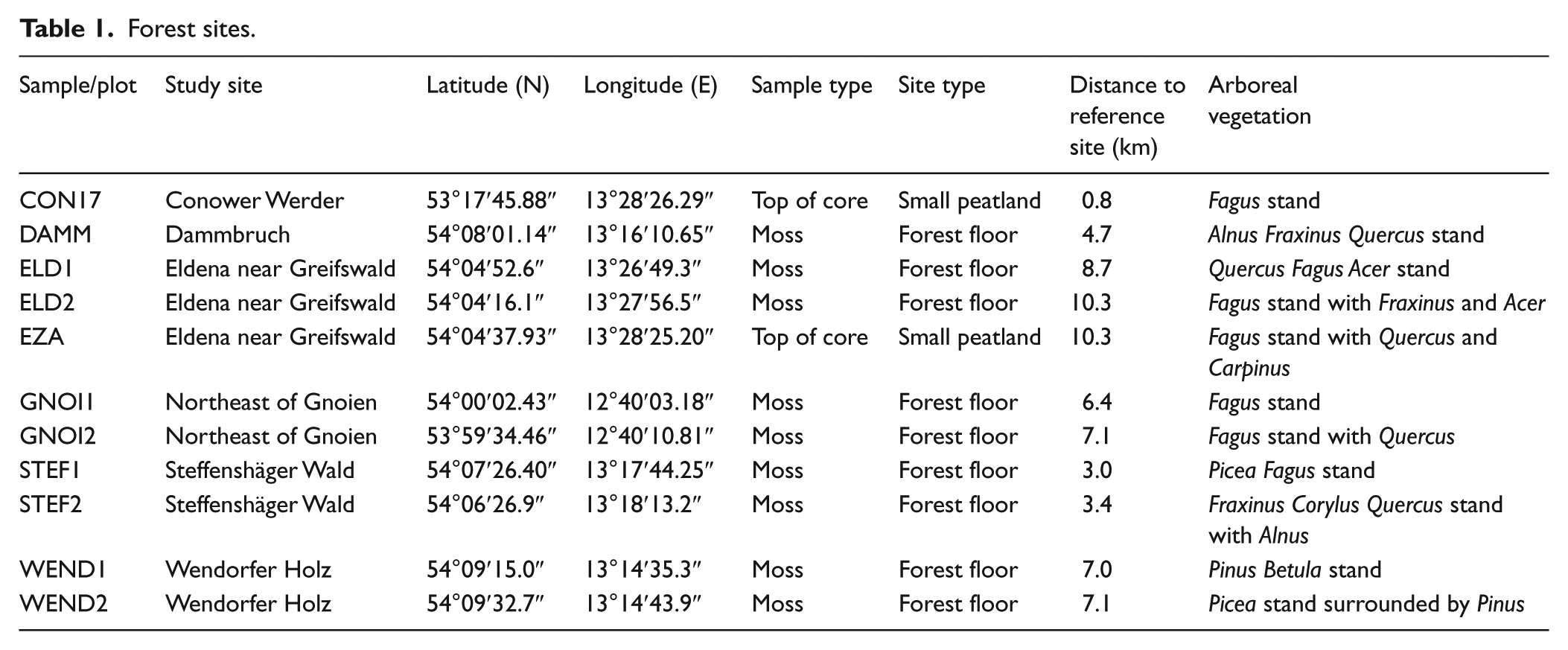
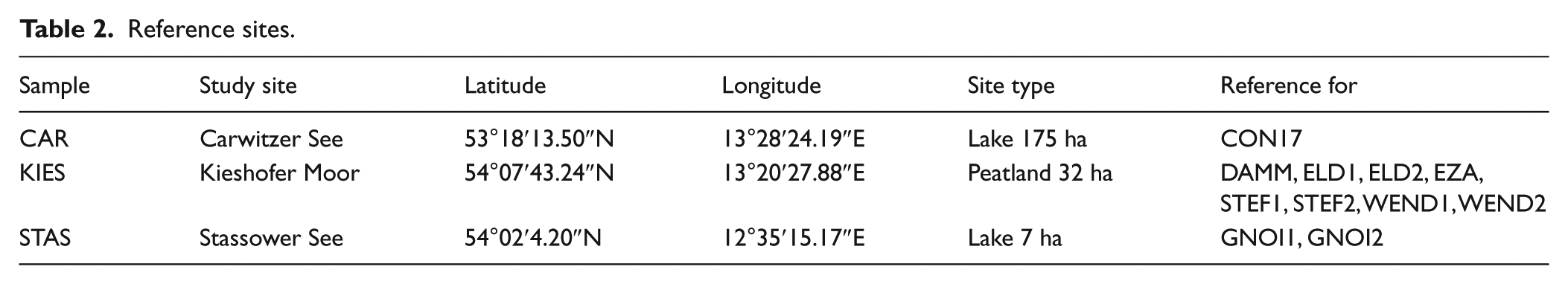
We studied 11 forest plots and 3 reference sites located in the federal state of Mecklenburg-Vorpommern in NE Germany (Tables 1 and 2). The lowland area is flat to slightly hilly and characterised by morainic plains, terminal moraines and outwash plains. The climate is temperate with a mean annual air temperature of 8.8°C and mean annual precipitation of 620 mm (1983–2013, German Meteorological Service DWD). The forest plots were selected to cover the variety of forest types found in the area (Table 1). Plots were placed at a distance of 150–650 m from the nearest forest edge. At each plot, tree and shrub cover was recorded and surface samples were collected for pollen analysis. In addition, we collected surface samples from three large basins close to the sampled forest plots to assess regional pollen deposition (Table 2).
Forest sites.
Reference sites.
Pollen analysis
Surface samples for pollen analysis were collected in the centre of each forest plot. In nine of the plots, mosses were sampled at the centre and corners of a 1-m2 area and mixed. The remaining two samples were taken from the surface of small peatlands (40 × 80 m for CON17 and 10 × 30 m for EZA; Table 1). In the ‘Kieshofer Moor’, a large open peatland, the upper 5 cm of Sphagnum moss was sampled, and in the lakes ‘Carwitzer See’ and ‘Stassower See’ the upper 3 cm of sediment was sampled using a gravity corer (Uwitec, Austria).
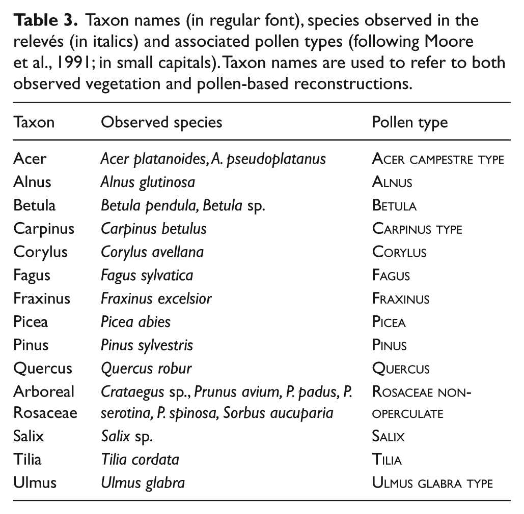
Pollen sample preparation (cf. Fægri and Iversen, 1989) included treatment with HCl, 10% KOH, sieving (120 µm) and acetolysis (7 min); samples rich in silicates were additionally treated with HF. Samples were mounted in silicone oil and counted with 400× magnification. In order to differentiate clearly between plant taxa and pollen types, the latter are displayed in Small Capitals (Table 3; Joosten and De Klerk, 2002). Pollen nomenclature follows Moore et al. (1991).
Taxon names (in regular font), species observed in the relevés (in italics) and associated pollen types (following Moore et al., 1991; in small capitals). Taxon names are used to refer to both observed vegetation and pollen-based reconstructions.
Tree and shrub cover
Forest vegetation relevés were made by estimating the crown cover of trees and shrubs of reproductive age (cf. Lang, 1994) in circular field plots of 100 m radius. Plots were subdivided into four 25-m-wide rings that were visually assessed in subsections. The obtained cover estimates were merged and normalised to a total of 100%. Taxon cover was estimated in steps of 5% – below 5% in steps of 1%. Cover below 1% was recorded by ‘+’ and ‘r’ (cf. Braun-Blanquet, 1964); for numerical analysis, these estimates were transformed to 0.5% and 0.15%, respectively.
Cover estimates were cross-checked using aerial orthophotos (GeoPortal.MV). Where reconstructed presence was not supported by the relevé, we used forest inventory data and additional field observations to check whether corresponding taxa were present within 2000 m distance from the sampling point. Whereas elements of the actual vegetation are written in Italics, reconstructed taxa are written in regular font (Table 3).
MARCO POLO
The MARCO POLO approach starts from the common assumption that regional pollen deposition (as recorded in large basins: our reference sites, Table 3) represents the vegetation composition of a larger area (Janssen, 1966). Pollen deposition in small basins (our forest sites, Table 2) deviates from this regional record, because it contains a large proportion of local and extra-local pollen (sensu Janssen, 1966), i.e. pollen produced by vegetation in and directly surrounding the basin. Like LRA (Sugita, 2007a, 2007b), MARCO POLO uses this difference to reconstruct vegetation composition at the stand scale (Spangenberg, 2008; cf. Jacobson and Bradshaw, 1981). The approach is a logical extension of the work of Andersen (1967, 1970), who found that pollen values increase linearly with local tree cover starting from a non-zero background value. This background pollen he identified as originating from the wider surroundings, i.e. from regional sources (sensu Janssen, 1966).
First step: Presence/absence analysis
In MARCO POLO, a ‘local’ pollen record from a small basin (L-record) and a contemporaneous ‘regional’ record from a neighbouring large basin (R-record) are used. For both records, percentage values are initially calculated based on a pollen sum that includes all pollen types of interest, using the same set of pollen types for both records. For each pollen value, the 1 sigma uncertainty range is calculated following Mosimann (1965). Pollen types for which the percentage value minus 1 sigma in the L-record is larger than its value plus 1 sigma in the R-record are considered to have an (extra-)local component in the L-record. These types are subsequently removed from the pollen sum of both the L- and the R-record, percentage values and uncertainty ranges are recalculated, and again the pollen types with (extra-)local values in the L-record are removed (Figure 1). This procedure is repeated until no further pollen types can be identified to have an (extra-)local component in the L-record. All pollen types still left in the pollen sum are considered regional (sensu Janssen, 1966; i.e. ‘exotic’ sensu Andersen, 1970) and yield an adjusted regional pollen sum that is free of disturbing (extra-)local factors (Janssen, 1959).
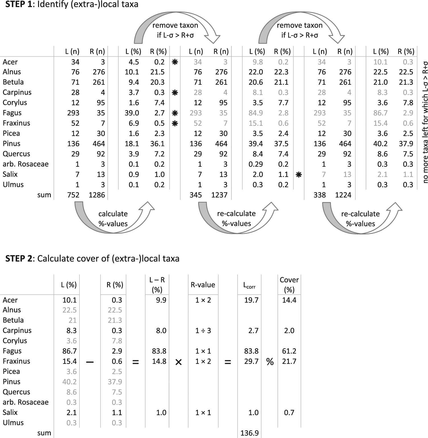
MARCO POLO explained using data from site ELD2. Step 1 (top) identifies taxa with an (extra-)local component in a ‘local’ L-record through comparison with a ‘regional’ R-record. In the first round, percentage values are calculated using a pollen sum that includes all types. Those pollen types for which the percentage value minus 1 sigma in the L-record is larger than the pollen value plus 1 sigma in the R-record (marked *) are removed from the pollen sum (in grey font). Percentage values of both the L- and R-record are recalculated based on this adjusted sum and further types may be removed in subsequent rounds until no types with an (extra-)local component are left. Step 2 (bottom) uses the percentage values resulting from Step 1 and calculates the difference between the L- and the R-record for each taxon with an (extra-)local component (now in black font). The result is a value for the (extra-)local component in the L-record. These values are multiplied by R-values and normalised to 100% cover.
After this identification of (extra-)local components, the pollen values calculated using this adjusted regional pollen sum serve as the basis for quantitative reconstruction of the (extra-)local vegetation in the second step of MARCO POLO.
Second step: Correction for differences in representation
Once pollen types with an (extra-)local component have been identified, the relative cover of the associated taxa is determined. At this stage, all pollen values are based on the adjusted regional sum. The pollen values of types with an (extra-)local component in the L-record are not free of a regional component; this regional component is removed by subtracting the pollen values in the R-record from the corresponding values in the L-record. The resulting values, which represent the (extra-)local components contained in the L-record only, are finally corrected using representation factors (R-values). To that end, each value is multiplied by the representation factor of the corresponding taxon. The resulting values are normalised to a total of 100%. The result is an estimate of the relative cover of each taxon in close vicinity to the sampling point.
We tested MARCO POLO by combining each of the 11 forest plots (as L-records) with the closest of the three reference sites (as R-records; Table 2). We used the R-values for arboreal taxa of Andersen (1970; Table 4). This large set of R-values was derived from extensive data gathered in a landscape with a similar glacial and species immigration history to our study area and similar physiographical features and climate regime. Moreover, the set includes Fagus, which is a dominant tree taxon in our study area. Thus far, R-values for arboreal Rosaceae and Salix have not been published for Northern and Central Europe. We used an arbitrary R-value of 1:1 to be able to include these taxa in the quantitative reconstruction. These values are close to the 0.8:1 R-value for ‘Others’ (Rosaceae, Ilex, Salix, etc.) of Davis (1963) for a study site in North America. The low pollen values associated with these taxa and the fact that they occur in a limited number of plots only did not allow for an in-depth analysis of the suitability of these values. For the same reasons, the error caused by the arbitrary setting will be small.
Correction factors applied in this study: R-values for MARCO POLO, and PPE and fall speed for LRA.
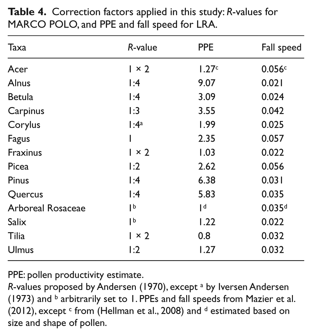
PPE: pollen productivity estimate.
R-values proposed by Andersen (1970), except a by Iversen Andersen (1973) and b arbitrarily set to 1. PPEs and fall speeds from Mazier et al. (2012), except c from (Hellman et al., 2008) and d estimated based on size and shape of pollen.
At plot CON17, Alnus trees (<5 m high) and Betula shrubs grow on the sampled peatland. Their presence in the area is restricted to this small peatland site. They show very high local pollen values that distort the reconstruction of the remaining taxa in both LRA and MARCO POLO. We therefore removed Alnus and Betula from the pollen record of CON17 and repeated the analyses.
LRA modelling
The LRA (Sugita, 2007a, 2007b) consists of two models: The REVEALS model translates pollen deposition from large sites into mean regional vegetation composition. The LOVE model then uses this result to translate pollen deposition from small sites into mean vegetation composition near these small sites. We applied the LRA by running the ‘REVEALS.v4.2.2.Tallinn.wks.exe’ and ‘LOVE.v3.1.7.Tallinn.wks.exe’ programs provided by S. Sugita. For each of the 11 forest plots we ran the LOVE model using REVEALS results from the closest of the three reference sites (Table 2). Besides pollen data, the LRA requires pollen productivity estimates (PPEs). We used the set of mean PPEs (‘PPE.st2’) compiled by Mazier et al. (2012), except for Acer (Table 4). For Acer, so far only two, substantially different PPEs are available from studies in Southern Sweden and Switzerland. We used the PPE from the less distant and physiographically similar Swedish study area.
Statistics
We compared observed and modelled plant cover values using regression analysis. Regression analysis was performed on the total set of data (pooled across all sites and taxa) and for each single taxon (pooled across all sites). Because both the observed and modelled values are subject to error, the ordinary least squares method would underestimate the true slope of the regression (Riggs et al., 1978). We therefore used the geometric mean method to estimate regression parameters (Riggs et al., 1978; Webb III et al., 1981). Regression analysis in all cases showed that the intercept did not differ significantly from 0. As zero cover would moreover logically result in zero (extra-)local pollen deposition, we decided to use regression analysis with zero-intercept. As all values are presented as percentage values, overestimation in one taxon will automatically result in underestimation of all other taxa. We will address this interacting effect of percentage values in the discussion section.
About 40% of plot STEF1 is covered by young Picea trees, which neither of the models was able to depict. Although we had assumed these trees were of reproductive age, they apparently were not. We therefore removed this taxon from the record before quantitative analysis.
Results
Presence/absence
We recorded 20 arboreal taxa in the relevés that are associated with 13 pollen types. These 13 pollen types plus Salix (Salix was not recorded in the relevés) were used in the analysis (Table 3). In total, 154 sets (11 plots × 14 taxa) of one observed and two reconstructed cover values were obtained.
MARCO POLO and the LRA perform similarly in reconstructing local presence/absence of taxa (Table 5). The presence was correctly reconstructed by both models in 56 cases (true-positives); absence in 45 (true-negatives).
Presence reconstructed by the LRA and MARCO POLO models for different taxa. The number of plots (radius 100 and 500 m) in which a taxon is present (N100 and N500) is compared with the number of plots at which local presence of the taxon was reconstructed by MARCO POLO (NMP) and the LRA (NLRA). Reconstructions are divided into true-positives (T) and false-positives (F). Improvement with greater radius is indicated by bold numbers.
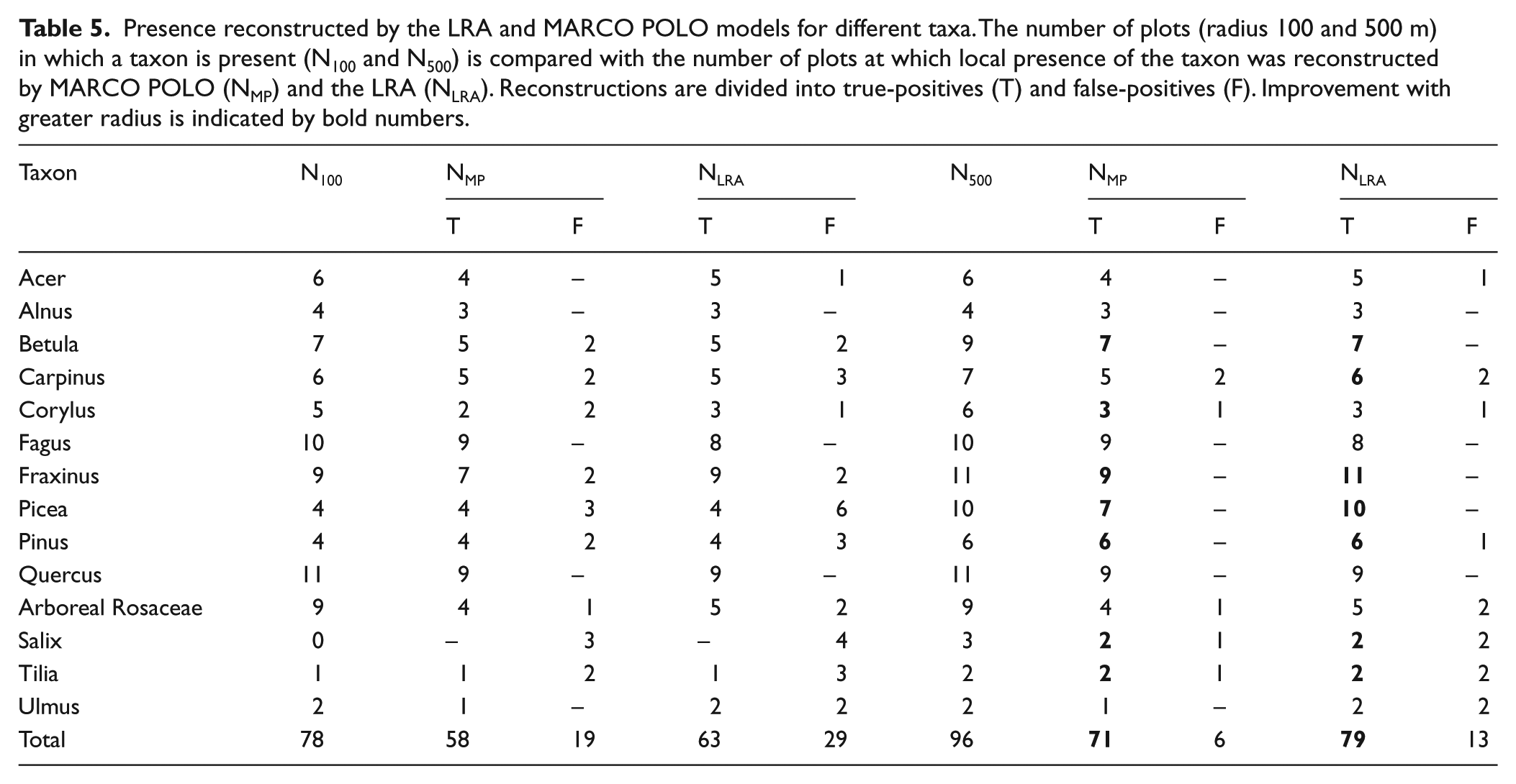
In 31 sets, at least one of the models reconstructed presence although the taxon was absent in the relevé (false-positives; Figure 2). In 27 of these 31 cases, the reconstructed values are only small (<3%). Of the 31 false-positives, 16 can be explained by the presence of a corresponding taxon within 500 m of the sample point. In the remaining sets, LRA produces 15 false-positives; MP only 8. In these 15 cases, the reconstructed cover is (well) below 2%. In 22 sets, at least one of the models indicated local absence, although the taxon was recorded in the relevé (false-negative). In all these cases, the cover of the taxon was below 2%.
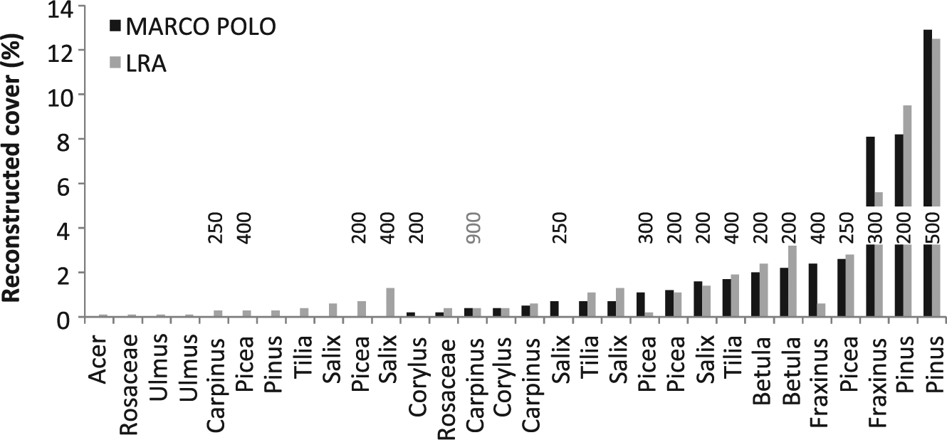
Reconstructed cover for cases where the respective taxon is actually absent in the relevé (100 m radius). Numbers denote the closest distance (m) from the sampling point at which the taxon was observed.
We thus end up with 109 sets of observed and corresponding model values with at least one value larger than 0. These sets are used in the subsequent analysis of cover values.
Reconstructed cover
MARCO POLO and the LRA perform well in reconstructing the cover of taxa within a 100-m radius (Figure 3). Regression analysis of the total of the 109 datasets for both models reveals a near-perfect fit between the reconstructed and observed cover (Table 6). The error of the LRA model (RMSE = 8.58%) is slightly higher than that of MARCO POLO (RMSE = 6.44%). Both models tend to overestimate the cover of rare taxa (cover ⩽10%); for higher values, error is more evenly distributed between over- and underestimations (Figure 4).
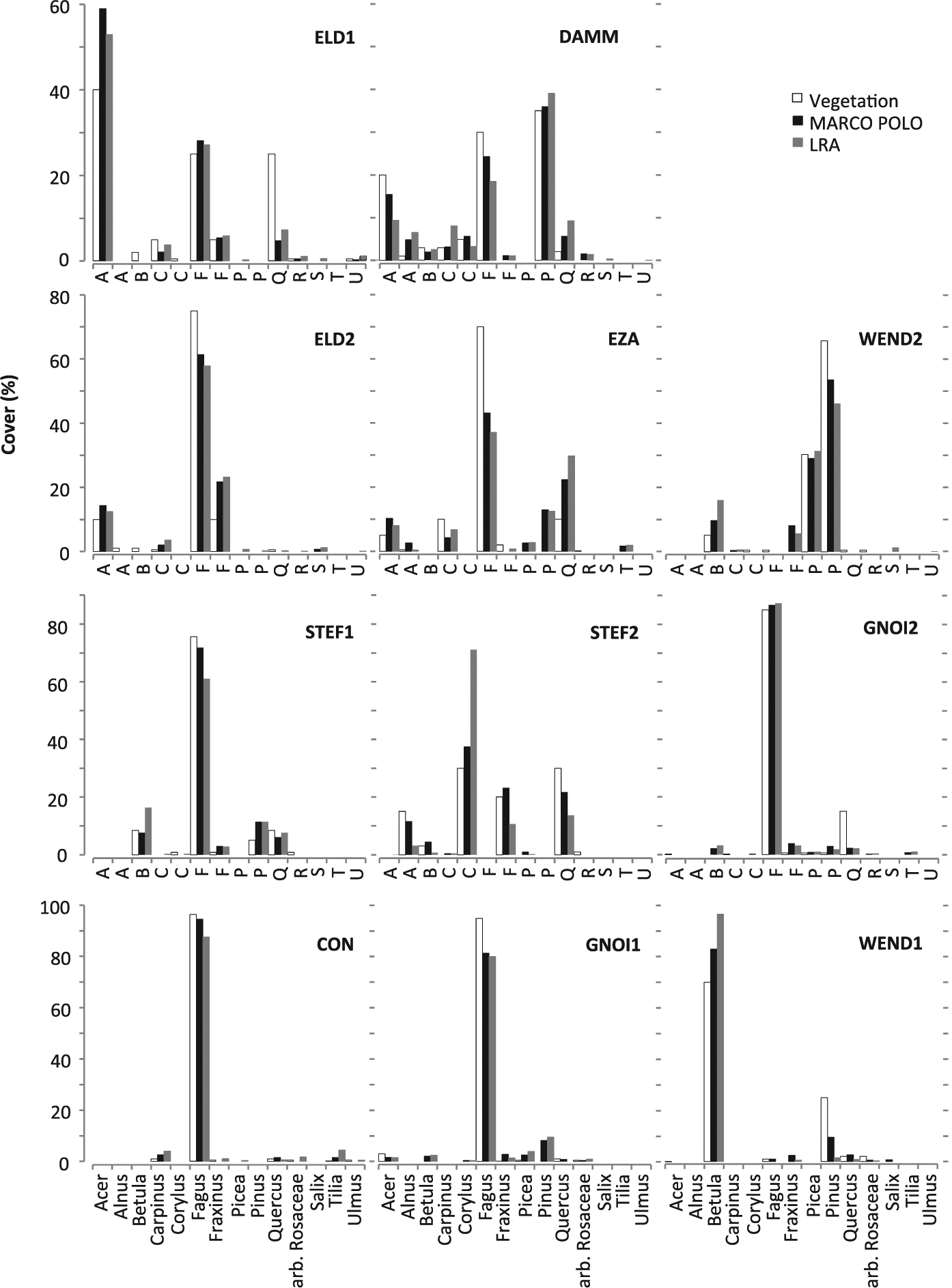
Observed and modelled cover for each plot and taxon. For plot codes, see Table 1.
Similarity between observed (Veg.) and modelled (LRA and MP) cover. Similarity is expressed as regression coefficient and coefficient of determination of a geometric mean linear regression and as root mean square error.
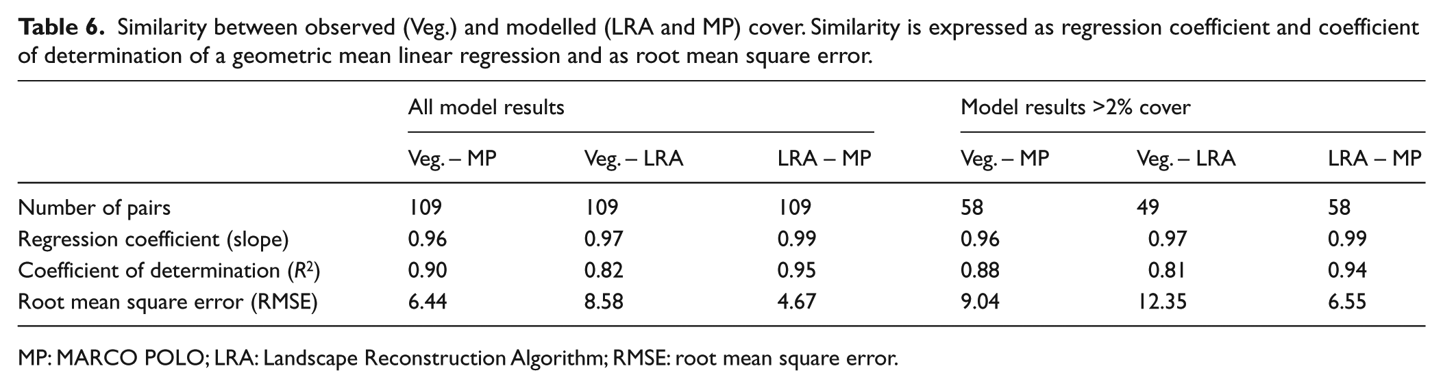
MP: MARCO POLO; LRA: Landscape Reconstruction Algorithm; RMSE: root mean square error.
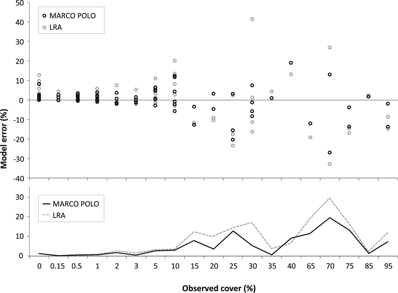
Error in reconstructed cover in relation to observed cover. Dots in the upper graph denote the difference between reconstructed and observed cover and dashed lines in the lower graph the RMSE. Note the scaling of the x-axis.
The performance of the models differs considerably between taxa (Table 7). Both models show close correlation (R2 > 0.65) between the observed and reconstructed cover for Fagus, Picea, Betula, Corylus, Acer and Alnus; MARCO POLO also for Fraxinus and Pinus. However, the cover tends to be overestimated (slope >1.2) in case of Corylus and Acer (in LRA also Betula) and underestimated (slope <0.8) in case of Alnus (in LRA also Pinus). The mismatch is particularly large in the LRA estimates for Corylus and Alnus. Correlation is weak (R2 < 0.65) for Quercus, Carpinus and arboreal Rosaceae.
Regression coefficient (slope) and coefficient of determination (R2) of taxon-specific geometric mean linear regression (with zero-intercept) between observed and reconstructed cover for MARCO POLO (MP) and LRA. Bold values indicate slopes close to 1 (0.8 < α < 1.2) and R2 > 0.65.
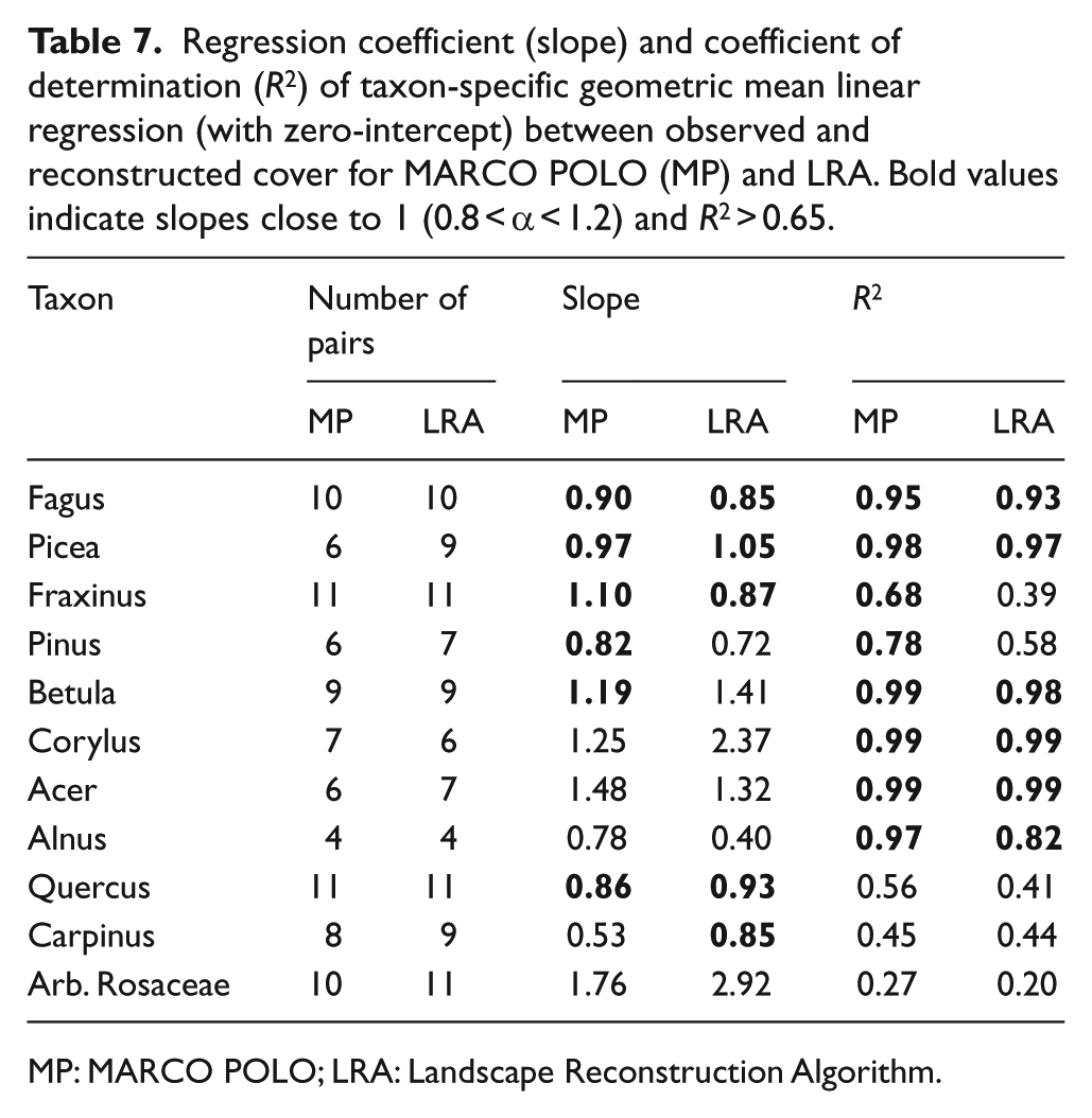
MP: MARCO POLO; LRA: Landscape Reconstruction Algorithm.
Discussion
The forest stand reconstructions of the MARCO POLO model are largely consistent with the observed tree cover and similar to the LRA reconstructions. Both MARCO POLO and LRA reliably reconstruct the presence of taxa with more than 2% cover.
MARCO POLO correctly reconstructs local presence in about 75% of the cases (Table 5). LRA performs slightly better at about 80%, but produces more false-positives: in 14% of the cases in which the LRA reconstructs local presence, the taxon is not present within a 500-m radius (<8% for MARCO POLO). However, falsely reconstructed presence is never above 1.3% cover for LRA (n = 12) and never above 0.7% for MARCO POLO (n = 5) (Figure 2).
Both models may fail to reconstruct the presence of rare taxa, resulting in false-negatives. In all these cases, the observed cover of the rare taxon was below 2%. Considering the false-positive thresholds of 1.3% and 0.7%, we propose a conservative 2% threshold: For both models, any reconstructed cover above 2% implies that a taxon is indeed present – if not nearby, then at least within a 500-m radius. A value below 2% may mean a taxon actually is not present locally. In case of reconstructed absence, a taxon may still have been present with a cover below 2%. Besides the 2% threshold, there is no apparent pattern in modelled presence/absence. One might expect that model errors are more common for entomophilous taxa or for taxa with low pollen productivity, but neither seems to be the case.
The 2% error made by the models in reconstructing presence/absence implies that error is equally small in reconstructing near-total dominance (cover close to 100%). In other words, very low and very high values are close to the ideal 1:1 regression between modelled and observed data. In addition, if the cover of a taxon is underestimated at a particular site, the other taxa at that site are overestimated because cover is expressed as percentage and always totals 100%. Thus, any deviation away from the 1:1 regression is accompanied by deviations of the same total size in the other direction. As a result, a regression that uses the total dataset of modelled and observed cover necessarily reveals a near-perfect 1:1 fit and is thus not a good measure for model performance. The general performance of the models should therefore be judged by the variance around the regression (R2) or the deviation from the 1:1 ideal (RMSE). MARCO POLO performs slightly better than the LRA in this respect. When the values below 2% are removed from analysis, R2 remains high for both models, but as can be expected when low values with low error are removed, RMSE values increase (by about 40%; Table 6).
The correction factors (R-values and PPEs) used in the models are mean values derived from field studies at multiple sites (Andersen, 1970; Mazier et al., 2012). Pollen load shows considerable variation in relation to stand structure (age, health, shading, productivity, patchiness, etc.) and site characteristics (relief, wind direction, air turbulences, etc.) (Matthias et al., 2012; Theuerkauf et al., 2013). Such variation (largely) averages out over large areas, which means that in quantitative reconstruction of regional vegetation, the use of the averaged correction factors is appropriate. However, it will cause error in reconstructions at the stand scale.
For example, Quercus is underrepresented in the model results of plots ELD1, GNOI2 and STEF2 (Figure 3). In these plots, Quercus trees are old and of poor vitality and presumably produce less pollen than the correction factors suggest. Picea is similarly underrepresented in plot STEF1; here probably because trees are not yet reproductively mature. In the case of plot CON17, Betula and Alnus growing in the small peatland at the centre of the plot provide so much pollen to the sample that the dominance of Fagus in the (much larger) relevé is obscured in the reconstruction (Figure 5). The local presence of Betula and Alnus results not only in a high local component from gravitational pollen deposition but the Betula shrubs at the sample point probably block the trunk space pollen component of the surrounding forest as well (Tauber, 1965). Such reconstruction errors in the percentage cover of one taxon necessarily cause error in other taxa as well, and do so in a non-linear way (the ‘Fagerlind effect’; Fagerlind, 1952; Prentice and Webb III, 1986). This type of error was very prominent in the plots STEF1 and CON17. When we removed the taxa that disturb the picture (Picea; Betula and Alnus) from the respective datasets, the reconstructions for the remaining taxa improved significantly.
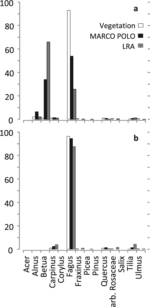
Observed and modelled cover for site CON17. Betula and Alnus are growing locally on this peatland site and disturb the reconstruction when included (a; total RMSE over all reconstructions is 30.26% for LRA and 16.58% for MARCO POLO); results are much better when the disturbing taxa are excluded (b; RMSE 3.64% for LRA and 1.05% for MARCO POLO).
A single correction factor can never capture the specific conditions of each site. This inherent error restricts the predictive capacity of stand-level reconstructions by default. A larger dataset would be needed to assess inherent variation and possibly derive general as well as taxon-specific error estimates. Because of the Fagerlind effect, error will be highest when the observed cover is near 50% (Figure 4). Whereas the inherent error cannot be reduced, bias caused by inappropriate correction factors can.
Close correlation between the reconstructed and observed cover (slope close to 1, high R2) suggests that correction factors are (near-)optimal for several taxa in our study: the R-values for Fagus, Picea, Betula, Fraxinus and Pinus used in MARCO POLO and the PPEs for Fagus and Picea used in the LRA (Table 7). For other taxa, the reconstructions appear to be biased. Both models tend to systematically overestimate the cover of Corylus and Acer – the LRA also of Betula – indicating that R-values are too high and PPEs too low. The opposite applies to Alnus. The remaining taxa show a poor fit between the modelled and observed cover. The observed cover of Carpinus and arboreal Rosaceae is low in all cases (⩽10% and ⩽2%, respectively) and any trend is apparently lost in the noise. Tilia and Ulmus occur with even lower cover and only in very few of the plots. Although higher cover was observed for Quercus (up to 35%), this taxon is known to show high variation in pollen–vegetation relationships, making derivation of a robust correction factor difficult (Andersen, 1970; Theuerkauf et al., 2013).
The R-values used in MARCO POLO are derived from closed forest settings similar to our own (Andersen, 1970). In contrast, the PPEs for the LRA have mostly been estimated using surface samples from (semi-)open settings (including lakes, heathlands and large forest openings; Mazier et al., 2012) to avoid (extra-)local overrepresentation of forest taxa. These PPEs may not be fully applicable to closed forests, because pollen dispersal is different. Whereas the canopy component dominates the pollen load of forest taxa arriving to open settings, the trunk space component is more important in closed forest settings (Tauber, 1965). As a result, representation of taxa forming lower canopy strata in the forest will differ between pollen samples taken inside and outside the forest. The pollen dispersal function that underlies the PPE.st2 data does not capture this difference, which for some taxa may, in part, explain the poor performance of the LRA compared with MARCO POLO. More sophisticated pollen dispersal models (e.g. Lagrangian stochastic models; Kuparinen et al., 2007) that are able to depict pollen dispersal both outside and inside the forest would be needed to produce accurate PPEs that are applicable both at the regional and the (extra-)local scales.
Any reconstruction of local forest cover faces the problem that a few trees close by may contribute as much pollen as many trees at a larger distance (Jacobson and Bradshaw, 1981; Oldfield, 1970). Moreover, different taxa have their distinct pollen production and dispersal characteristics so that delineating a common (extra-)local source area for a site is always deficient (Jackson, 1990; Jacobson and Bradshaw, 1981). Despite these limitations, several studies have shown that pollen data from small forest sites (soils, small ponds, small peatlands) best represent forest composition within 30–150 m radius (Andersen, 1970; Bunting et al., 2005; Calcote, 1995; Sugita, 1994; Sugita et al., 2010). Our results support these findings.
In only a few cases, species are reconstructed to be locally present with a cover larger than the 2% threshold although they are absent within the 100-m radius (Figure 2). At plot GNOI1, for example, the presence of pine in the local reconstruction can be attributed to a large pine plantation beginning about 200 m distance from the sampling point. In WEND2, the presence of Fraxinus at about 300 m distance can hardly explain the high reconstructed cover. Here, the high number of pollen must have been deposited in previous years before large numbers of trees were lost because of ash dieback (cf. Pautasso et al., 2013). Similarly, large pine trees were cut near plot EZA some years before sampling. These few problems aside, we find good correlation between the pollen-based reconstructions and the plant cover within a 100-m radius.
Like the LRA, the application of MARCO POLO to palaeo-data requires robust chronological linkage between the L- and R-records. Once this synchronicity is established, insight can be gained into long-term vegetation dynamics at small spatial scales; using a combination of sites, spatial patterns and shifting mosaics can be detected (Spangenberg, 2008). In this way, records of (extra-)local pollen (L-records) can help understand the fine-scale patterns and processes that underlie large, landscape-level dynamics of, for example, plant migration and land use. L-records can be found in terrestrial soils (including palaeosoils buried by, for example, peatlands, dunes or earthworks), in small ponds or peatlands and near the edges of larger peatlands or lakes.
The first step of MARCO POLO, in which only (extra-)local presence or absence of taxa is assessed, does not require R-values. Close vicinity to the sample point can thus be reconstructed also for the numerous herbs and especially cultivated plants, for which R-values are thus far lacking. Such presence/absence analyses may be particularly worthwhile in reconstructing (extra-)local vegetation cover in archaeological settings, for example, revealing where particular crops were grown or in which rotation.
Conclusion
Both MARCO POLO and the LRA are able to reconstruct the presence or absence of taxa at the stand scale within a small margin of error. Reconstructed cover values below 2% are not reliable and should be interpreted with caution. Statistical reliability, possible contamination or re-deposition, long distance transport and ecological plausibility should be taken into account when drawing conclusions from low values.
MARCO POLO explicitly reconstructs presence/absence in its first step, solely on the basis of pollen values. The LRA is more complex and requires correction factors (PPEs, fall speed) and a dispersal model to deliver results. However, the reconstruction of presence/absence hardly depends on the validity of these model attributes. At this stage, both models produce reliable results and can be applied to reconstruct the species composition of plant communities for which no modern analogue exists.
The full effect of model attributes (R-values in MARCO POLO and PPEs, fall speeds and dispersal model in the LRA) and their validity only becomes noticeable in the taxon-specific performance of the models. Although some model parameters evidently need revision, the present first test shows that the simple correlative approach of MARCO POLO performs at least as well as the complex LRA model. The dispersal model of the LRA (that underlies the PPEs) seems to be the most critical component.
MARCO POLO relies on R-values derived from ‘simple’ linear correlation of pollen and vegetation proportions, which makes it transparent and easy to implement. Studies into (non-distance-weighted) R-values have become virtually non-existent since the introduction of the LRA. Our results show that it is definitely worthwhile to revive research into R-values.
Model performance may be impaired in small peatland sites. If taxa of interest are growing on the site itself (e.g. Alnus, Betula, Calluna, Cyperaceae, Pinus, Poaceae, Salix), this may distort the pollen record. Such local presence may be inferred from macrofossils, from the presence of unripe, not-yet separated pollen (pollen clumps) or from exceptionally high values of the (extra-)local component. When using small peatland sites, any taxon that may have been growing on the peatland should be excluded from the final quantitative reconstruction. However, on the surrounding mineral ground, the same taxa may act as pioneer species or may be indicative for openness or early successional stages – all of interest to ecologists. Additional indicators, such as pollen of co-occurring taxa, non-pollen palynomorphs, charcoal or geochemical parameters, and expert judgement are then required to draw conclusions. In that sense, models are only an aid to reconstruct past stand-scale vegetation. They cannot replace the ecological expertise of the interpreter.
Footnotes
Acknowledgements
AM carried out the field work and pollen analysis and did the MARCO POLO calculations. AM and HJ developed the idea behind the MARCO POLO model, which AM implemented. MT analysed the forest inventory data and did the LRA calculations. AM and JC analysed the model outcomes and wrote the paper, to which MT and HJ contributed. We thank Uwe Gehlhar (Research Institute of the State Forest Authorities of Mecklenburg-Vorpommern) for supporting data collection from sites CON17 and CAR, thus helping us to further develop MARCO POLO. We also thank an anonymous reviewer for helpful comments. We dedicate this paper to the memory of Roel Janssen for his pioneering work and inspirational ideas.
Funding
The work was supported by the Research Institute of the State Forest Authorities of Mecklenburg-Vorpommern, the Hemholtz Association (ICLEA VH-VI-415) and a PhD scholarship of the Heinrich Boell Foundation.