A late-Holocene multi-proxy record from the northern Norwegian margin: Temperature and salinity variability

Abstract

To elucidate the natural variability of Atlantic and Coastal water, a late-Holocene multi-proxy analysis is performed on a marine sediment core from the northern Norwegian margin. This includes planktic foraminiferal fauna and their preservation indicators, stable isotopes (δ¹⁸O_c, δ¹³C), sub-surface temperature (SST_Mg/Ca) and salinity (SSS) records based on paired Mg/Ca and δ¹⁸O_c measurements of Neogloboquadrina pachyderma and transfer function–derived sub-surface temperatures (SST_Transfer). The record shows a general cooling with subtle fluctuating palaeoceanographic conditions, here attributed to shifting North Atlantic Oscillation (NAO) modes. Period I (ca. 3500–2900 cal. yr BP) is strongly influenced by Coastal water and stratified water masses, possibly correlating to negative NAO conditions. During period II (ca. 2900–1600 cal. yr BP), dominating warm Atlantic water might be linked to a positive NAO mode and the Roman Warm Period. A renewed influence of Coastal water is observed throughout period III (ca. 1600–900 cal. yr BP). Stable and colder SST values potentially correlate to the Dark Ages and are here attributed to negative NAO conditions. Within period IV (ca. 900–550 cal. yr BP), the core site experienced a stronger influence of Atlantic water which might be because of the positive NAO conditions correlating to the ‘Medieval Warm Period’. Additionally, an inverse correlation in Atlantic water influence between the eastern and western Atlantic Ocean is observed throughout periods II, III and IV. This Atlantic oceanographic see-saw pattern is attributed to an opposite climatic response to changing NAO conditions arguing for a coupling between ocean and atmosphere.

Keywords

Atlantic water influence Coastal water late-Holocene multi-proxy record NAO northern Norwegian margin

Introduction

Throughout the late-Holocene, a general cooling trend has been observed in the North Atlantic associated with a reduced influence of warm Atlantic water (e.g. Hald et al., 2007; Skirbekk et al., 2010; Slubowska et al., 2005). A similar cooling trend, recorded by lake and tree records from north-western Europe, has been ascribed to reduced insolation at high latitudes (e.g. Bjune et al., 2009; Kaufman et al., 2009). In contrast, fluctuations of a strengthened Atlantic water inflow towards the Arctic Ocean have been observed for the Vøring plateau (e.g. Andersson et al., 2003, 2010; Risebrobakken et al., 2003), the Barents Sea (e.g. Berben et al., 2014; Duplessy et al., 2001; Lubinski et al., 2001) and the Svalbard margin (e.g. Jernas et al., 2013; Slubowska-Woldengen et al., 2007; Werner et al., 2013; Zamelczyk et al., 2013). Furthermore, throughout the late-Holocene, several observations of fluctuating climatic conditions have been found in the Nordic Seas (e.g. Giraudeau et al., 2004; Nyland et al., 2006; Slubowska-Woldengen et al., 2007; Solignac et al., 2006) as well as in north-western Europe (e.g. Bjune and Birks, 2008; Lauritzen and Lundberg, 1999). These include the ‘Roman Warm Period’ (RWP; ca. BCE 50–CE 400), the ‘Dark Ages’ (DA; ca. CE 400–800), the ‘Medieval Warm Period’ (MWP; CE 900–1500) and the ‘Little Ice Age’ (LIA; ca. CE 1500–1900; e.g. Lamb, 1977). As Atlantic water inflow towards the Arctic Ocean is part of the Atlantic Meridional Overturning Circulation (AMOC), it is not only contributing to climatic conditions in north-western Europe but also affecting the global climate system (e.g. Vellinga and Wood, 2002).

These fluctuating conditions have been ascribed to different causes such as solar forcing, volcanic eruptions (e.g. Bryson and Goodman, 1980; Jiang et al., 2005; Lean, 2002; Wanner et al., 2008) or changes in atmospheric forcing linked to the North Atlantic Oscillation (NAO) which influence the inflow of Atlantic water to the Arctic Ocean (e.g. Olsen et al., 2012; Trouet et al., 2009). Additionally, NAO fluctuations have also been suggested to result in opposite climatic trends between the subpolar North Atlantic and the Norwegian Sea during the late-Holocene (Miettinen et al., 2011, 2012).

Warm and salty Atlantic water is brought into the Nordic Seas by the North Atlantic Current (NAC) which flows parallel with colder and less saline Coastal water along the Norwegian margin. These two water masses possess opposite characteristics with respect to temperature and salinity. Furthermore, they respond opposite to the strengthened or reduced westerlies attributed to positive or negative NAO modes (e.g. Sætre, 2007). A positive versus negative NAO mode affects the climatic conditions in north-western Europe by generating warmer and wetter versus colder and dryer conditions (e.g. Wanner et al., 2001). Along the Norwegian coast, the impact of the variable NAO is seen in precipitation, temperature and wind intensity changes (Ottersen et al., 2001). Thus, the northern Norwegian margin is a key location to investigate the natural variability of Atlantic water inflow throughout the late-Holocene linked to fluctuating NAO modes.

For the Nordic Seas, several studies have reconstructed water mass properties based on planktic foraminiferal fauna. Transfer functions reflect sub-surface temperatures (SSTs), whereas stable oxygen isotopes reflect both the temperature and the stable oxygen isotopic composition of ambient sea water (δ¹⁸O_w; e.g. Berben et al., 2014; Rasmussen and Thomsen, 2010; Risebrobakken et al., 2003). In addition, paired calcite δ¹⁸O_c and Mg/Ca measurements enable the reconstruction of a palaeo SST and sub-surface salinity (SSS) record (e.g. Elderfield and Ganssen, 2000; Elderfield et al., 2010; Kozdon et al., 2009; Mashiotta et al., 1999; Thornalley et al., 2009).

In this study, the distribution of planktic foraminiferal fauna in a marine sediment core from the northern Norwegian margin is presented. Additionally, the preservation conditions as well as paired Mg/Ca and stable isotope (δ¹⁸O_c, δ¹³C) measurements of Neogloboquadrina pachyderma have been analysed by Berben (2014). This multi-proxy dataset represents the variability of both palaeo SST and SSS values. Hence, it is analysed in order to investigate the fluctuating interplay of Atlantic and Coastal water related to variable NAO modes throughout the late-Holocene.

Present-day oceanography

The Norwegian Sea is dominated by relatively warm and saline Atlantic water (>2°C, >35‰; Hopkins, 1991). Atlantic water is brought to the area by the two-branched Norwegian Atlantic Current (NwAC; Orvik and Niiler, 2002; Figure 1a). Both branches follow a topographically steered northward pathway through the Nordic Seas and eventually reach the Arctic Ocean via the Fram Strait. The eastern branch passes through the Faroe-Shetland channel and continues a pathway along the Norwegian shelf edge towards the Arctic Ocean with a branch flowing into the Barents Sea (Orvik and Niiler, 2002; Figure 1a). The western branch crosses the Iceland-Faroe Ridge entering the Norwegian Sea as the Iceland-Faroe frontal jet (Perkins et al., 1998; Figure 1a). Variability in the lateral (east-west) extent of the NwAC is mainly controlled by the intensity of the westerly winds associated with the NAO. In particular, an increased/decreased NAO index leads to a narrower/broader current (Blindheim et al., 2000). In addition, south of Iceland, Atlantic water is transported south-westwards by the Irminger Current (IC) where it is then incorporated into the West Greenland Current (WGC; Hopkins, 1991; Hurdle, 1986; Figure 1a).

Figure 1.

Study area of W00-SC3 (67.24°N, 08.31°E; circle) with the main surface currents: Norwegian Atlantic Current (NwAC), Irminger Current (IC), West Greenland Current (WGC) and Norwegian Coastal Current (NCC). (a) Surface currents presented on a bathymetric map. (b) Generalized schematic profile across the northern Norwegian margin modified after Rørvik et al. (2010). Coastal water (CW), Atlantic water (AW), Atlantic intermediate water (AIW) and Deep water (DW). (c) Detail map of the surface currents nearby the core site modified after Sætre (2007). Full and dotted arrows indicate Atlantic and Coastal water, respectively.

The Norwegian Coastal Current (NCC) transports Coastal water (2–13°C, 32–35‰; Hopkins, 1991) northwards originating from the North Sea, the Baltic and the Norwegian coast (Figure 1a). Coastal water is characterized by its low salinities because of the influence of freshwater runoff from the Norwegian mainland. The NCC is density driven which is mainly influenced by its salinity distribution (Sætre, 2007). Mixing with Atlantic water increases northwards, and thus, salinity increases whereas stratification reduces. In general, cold Coastal water can be found above warmer Atlantic water in the upper 50–100 m of the water column as a thinning wedge westwards (Ikeda et al., 1989; Figure 1b). A boundary is formed as a well-defined oceanic front between the cold, low-salinity Coastal water and the warmer, more saline Atlantic water (Ikeda et al., 1989). The overall properties and movements of the NCC are influenced by several factors such as freshwater, tides, wind conditions, bottom topography and Atlantic water (Sætre, 2007). In the study area, the topography causes the NCC to extend much further westwards and hence closer to the influence of the NwAC (Figure 1c).

Materials and methods

For this study, a marine sediment core from the northern Norwegian margin (Vøring plateau in front of Trænadjupet south of the Lofoten) was investigated. The core (W00-SC3; 67.24°N, 08.31°E) was retrieved in 2000 by the SV Geobay at a water depth of 1184 m (Laberg et al., 2002; Figure 1). Its recovery was 385 cm from which the top 19 cm was disturbed and therefore not used. The core consists of very soft clay sediments (Laberg et al., 2002) and was sampled for every centimetre between 19 and 263 cm.

Chronology

A depth–age model of W00-SC3 based on four AMS ¹⁴C dates measured on N. pachyderma was developed (Table 1). All four AMS ¹⁴C dates were calibrated using Calib 7.0.0 software (Stuiver and Reimer, 1993), the Marine13 calibration curve (Reimer et al., 2013) and a local reservoir age (ΔR value) of 71 ± 21 following Mangerud et al. (2006). The calibration was constrained on a 2σ range for both calendar years Before Present (cal. yr BP) and calendar years Before Common Era/Common Era (cal. yr BCE/CE). For this study, the cal. yr BP depth–age model will be used; however, the cal. yr BCE/CE scale was added for all plotted data in order to compare with different studies. The AMS ¹⁴C date at 23.5 cm was omitted from the final depth–age model as it appeared too old. The new depth–age model was constrained using a linear interpolation between the dated levels. Furthermore, based on the homogeneous lithology throughout the core, the sedimentation rate from 120 to 40 cm was extrapolated towards the top, more specifically between 40 and 19 cm (Figure 2). The resulting depth–age model is constrained between 3485 and 550 cal. yr BP (1536 BCE–1395 CE) and shows sedimentation rates between 0.79 and 0.87 mm/yr enabling a multi-decadal temporal resolution (Figure 2). Nonetheless, because of the low number of AMS ¹⁴C dates of this age model, the final interpretation is focused on a centennial temporal resolution.

Table 1.

AMS ¹⁴C dates and calibrated radiocarbon ages of W00-SC3. The calibration is performed using Calib 7.0.0 software (Stuiver and Reimer, 1993), the Marine13 calibration curve (Reimer et al., 2013) and a local reservoir age (ΔR value) of 71 ± 21 following Mangerud et al. (2006). The AMS ¹⁴C date highlighted in grey is omitted from the final depth–age model.

Lab ID	Core depth (cm)	Material	Uncorrected ¹⁴C age	Cal. yr BP	2σ range BP	Cal. yr BCE/CE	2σ range BCE/CE	Reference
Beta-334422	23.5	N. pachyderma	1590 ± 30	1069	968–1170	881 CE	780–982 CE	This study
TUa-2931	40.0	N. pachyderma	1360 ± 65	821.5	684–959	1128.5 CE	991–1266 CE	Laberg et al. (2002)
TUa-2930	120.0	N. pachyderma	2305 ± 55	1836	1688–1984	114.5 CE	35 BCE–262 CE	Laberg et al. (2002)
TUa-2929	263.0	N. pachyderma	3660 ± 95	3484.5	3237–3732	1535.5 BCE	1783–1288 BCE	Laberg et al. (2002)

Figure 2.

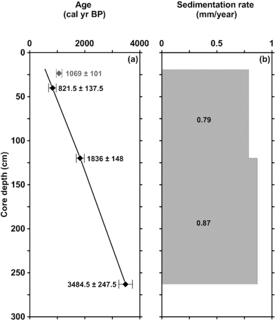
Depth–age model of W00-SC3 based on four calibrated AMS ¹⁴C dates. The 2σ range of the calibrated radiocarbon ages is indicated by an error bar. The exact values are noted in black for the used dates and grey for one omitted AMS ¹⁴C date. (a) Calibrated calendar years BP versus core depth; (b) sedimentation rates versus core depth.

Sub-surface water mass properties

All samples were freeze-dried, wet-sieved through three different size fractions (1000, 100 and 63 µm) and subsequently dried at 40°C. In total, 62 samples from every 4 cm from the 100–1000 µm size fraction were analysed for their planktic foraminiferal content (>300 specimens) following Knudsen (1998). The identification of left and right coiling N. pachyderma was done following Darling et al. (2006), meaning that the right coiling form is identified as Neogloboquadrina incompta (Cifelli, 1961). Subsequently, relative abundances (%) of each species, planktic foraminiferal concentration (#/g sediment) and fluxes (#/cm²/yr) were calculated. For the latter, a theoretical value for the dry bulk density of 0.76 g/cm³ was assumed based on marine sediment core T-88-2 retrieved nearby the study site (Aspeli, 1994) and subsequently calculated according Ehrmann and Thiede (1985).

Carbonate dissolution might affect the planktic foraminiferal assemblages; hence, it is necessary to investigate the preservation conditions in order to assess the potential dissolution-induced pre- and post-depositional alterations (e.g. Zamelczyk et al., 2013). Preservation indicators such as the mean shell weight (µg) of N. pachyderma (118 samples; Barker and Elderfield, 2002; Beer et al., 2010; Broecker and Clark, 2001) and fragmentation (%) of planktic foraminiferal tests (62 samples; Conan et al., 2002) were investigated. The latter was calculated using the equation of Pufhl and Shackleton (2004). For the mean shell weight, four-chambered, square-shaped and visually well-preserved forms from the same morphotype, combined with an optimum sample size of 50 specimens, were selected from a narrow size range (150–250 µm) in order to minimize problems of size and/or ontogeny variations (Barker et al., 2004; Broecker and Clark, 2001). Additionally, the weight percentages (wt. %) of total carbon (TC) and total organic carbon (TOC) were analysed for 244 samples. Subsequently, the calcium carbonate content (CaCO₃) in weight percentages (wt. %) was calculated following Espitalié et al. (1977).

Sub-surface water mass properties such as temperature and salinity, as well as primary production and stratification characteristics, are reflected by the stable oxygen and carbon isotopic compositions of foraminiferal calcite (e.g. Katz et al., 2010; Spielhagen and Erlenkeuser, 1994). From the W00-SC3 sediment core, 117 stable isotope (δ¹⁸O_c, δ¹³C) measurements (‰ vs VPDB) were carried out using N. pachyderma from the 150–250 µm size fraction. The measurements were performed with a Finnigan MAT 253 mass spectrometer coupled to an automated Kiel device at the Geological Mass Spectrometer (GMS) Laboratory of the University of Bergen. Analytical errors are, respectively, ±0.06‰ and ±0.03‰ for δ¹⁸O_c and δ¹³C measurements. Furthermore, a vital effect of 0.6‰ was applied on the δ¹⁸O_c measurements following previous studies from the area (Nyland et al., 2006; Simstich et al., 2003).

Quantitative reconstructions of summer SSTs (°C) at 100 m water depth (SST_Transfer) was done using a WA-PLS transfer function and a modern analogue dataset based on the >100 µm size fraction (Husum and Hald, 2012). Furthermore, reconstructions of both SST (SST_Mg/Ca) and SSS were based on a combined analysis of the Mg/Ca ratio (mmol/mol) and stable oxygen isotopic composition (δ¹⁸O_c) of N. pachyderma (Berben, 2014). In order to calculate the SST_Mg/Ca record (°C), the species-specific temperature:Mg/Ca equation of Kozdon et al. (2009) was used, whereas to calculate SSS values (‰), the salinity to δ¹⁸O_w relation by Simstich et al. (2003) was applied.

Results

Planktic foraminifera

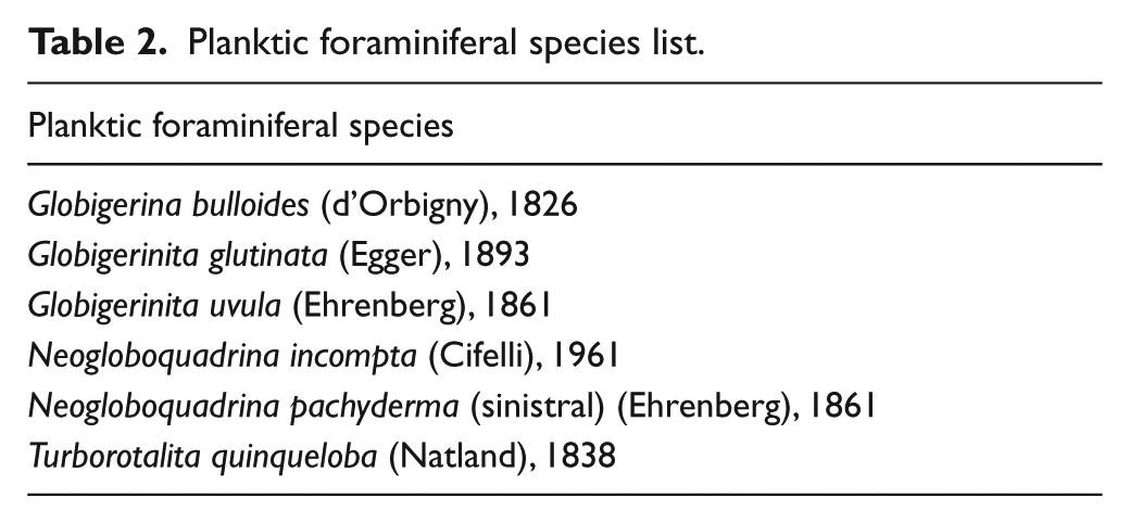
The planktic foraminiferal fauna consist of six species: N. pachyderma, Turborotalita quinqueloba, N. incompta, Globigerinita glutinata, Globigerina bulloides and Globigerinita uvula (Table 2; Figure 3). Overall, the record is dominated by N. incompta and T. quinqueloba with a mean value of ca. 34% and 29%, respectively (Figure 3c and d).

Table 2.

Planktic foraminiferal species list.

Planktic foraminiferal species
Globigerina bulloides (d’Orbigny), 1826
Globigerinita glutinata (Egger), 1893
Globigerinita uvula (Ehrenberg), 1861
Neogloboquadrina incompta (Cifelli), 1961
Neogloboquadrina pachyderma (sinistral) (Ehrenberg), 1861
Turborotalita quinqueloba (Natland), 1838

Figure 3.

Planktic foraminiferal fauna versus cal. yr BP (left y-axis) and cal. yr BCE/CE (right y-axis). The black diamonds on the y-axis indicate the AMS ¹⁴C converted to calibrated radiocarbon ages. (a) Planktic foraminiferal concentration (black) and flux (grey) versus age. (b–g) Species-specific relative abundances (black) and fluxes (grey) of planktic foraminifera versus age. (h) Transfer function–derived SST_Transfer record using a modern foraminiferal dataset by Husum and Hald (2012) versus age.

Between ca. 3500 and 2900 cal. yr BP, the planktic foraminiferal concentration and flux show relatively low values of ca. 563 #/g sediment and ca. 41 #/cm²/yr, respectively (Figures 3a and 4e). N. pachyderma and N. incompta show a decrease from ca. 18% to 12% and from ca. 40% to 19% (Figure 3b and c). Simultaneously, T. quinqueloba and G. uvula increase from ca. 28% to 36% and from ca. 5% to 21% (Figure 3d and g).

Figure 4.

Preservation and geochemical analysis versus cal. yr BP (left y-axis) and cal. yr BCE/CE (right y-axis). The black diamonds on the y-axis indicate the AMS ¹⁴C converted to calibrated radiocarbon ages. (a) Planktic foraminiferal fragmentation versus age. (b) Mean shell weight of N. pachyderma versus age. (c) Total organic carbon versus age. (d) Calcium carbonate versus age. (e) Planktic foraminiferal concentration (black) and flux (grey) versus age.

Both the planktic foraminiferal concentration and flux show slightly higher values of ca. 948 #/g sediment and ca. 63 #/cm²/yr, respectively, between ca. 2900 and 2300 cal. yr BP, and are followed by a sharp increase (Figures 3a and 4e). The highest recorded values in this study (3765 #/g sediment and 226 #/cm²/yr) are reached just before ca. 1600 cal. yr BP (Figures 3a and 4e). At ca. 1600 cal. yr BP, a profound decrease in planktic foraminiferal concentration and flux is noticed, showing a drastic change from high to relatively low values (from 3765 to 865 #/g sediment and from 226 to 52 #/cm²/yr, respectively). Furthermore, between ca. 2900 and 1600 cal. yr BP, the abundances of N. pachyderma are relatively stable around 12%, N. incompta shows high and stable values of ca. 33% and T. quinqueloba also shows high values (ca. 31%) albeit with a moderate decrease towards ca. 1600 cal. yr BP (Figure 3b–d). G. glutinata and G. bulloides show, in particular between ca. 2900 and 2300 cal. yr BP, the highest recorded values of this study (5% and 4%) followed by slightly reduced values towards ca. 1600 cal. yr BP (Figure 3e and f).

At ca. 1600 cal. yr BP, the strong shift from high to low planktic foraminiferal concentration and flux is followed by stable values between ca. 1600 and 900 cal. yr BP (ca. 1330 #/g sediment and ca. 80 #/cm²/yr; Figures 3a and 4e). In addition, the relative abundances of G. glutinata and G. uvula increase from ca. 2% to 4% and from ca. 15% to 27%, respectively (Figure 3e and g). Further throughout this time interval, T. quinqueloba shows a slight decrease from ca. 25% to 20% (Figure 3d), whereas the abundances of the remaining species stay relatively constant (Figure 3b, c and f).

Between ca. 900 and 550 cal. yr BP, the concentration and flux records slightly decrease towards 450 #/g sediment and 27 #/cm²/yr, respectively (Figures 3a and 4e). Most interesting in the faunal record is the clear decreasing shift in G. uvula starting at ca. 900 cal. yr BP (Figure 3g). Its relative abundance decreases from ca. 27% towards ca. 8% between ca. 900 and 550 cal. yr BP (Figure 3g). Simultaneously, N. pachyderma and N. incompta show the opposite shift towards values up to ca. 23% and 42%, respectively, at the top of the record (Figure 3b and c).

Preservation indicators

Between ca. 3500 and 2900 cal. yr BP, the planktic foraminiferal fragmentation shows generally high values around ca. 74%, whereas the mean shell weight of N. pachyderma varies around ca. 3.3 µg (Figure 4a and b). The fragmentation remains relatively stable around slightly reduced values (ca. 68%) between ca. 2900 and 1600 cal. yr BP (Figure 4a). At ca. 2900 cal. yr BP, the mean shell weight decreases towards 1.7 µg at ca. 2300 cal. yr BP whereafter an increase reaching ca. 3 µg is followed at ca. 1600 cal. yr BP (Figure 4b). Between ca. 1600 and 900 cal. yr BP, the mean shell weight remains stable around slightly reduced values of ca. 2.6 µg. Both preservation indicators show a pronounced increase from ca. 75% to 90% and from 2.4 to 3.2 µg between ca. 900 and 550 cal. yr BP (Figure 4a and b).

Geochemical analysis

Both TOC and CaCO₃ records show, between ca. 3500 and 2900 cal. yr BP, an increase of ca. 0.7 to 1.0 wt. %for TOC and ca. 17 to 22 wt. %for CaCO₃ (Figure 4c and d). Towards ca. 2300 cal. yr BP, increasing TOC values reach 1.1 wt. %whereafter a sudden drop to 0.8 wt. %is followed around ca. 2200 cal. yr BP (Figure 4c). Furthermore, this record remains stable around this value towards ca. 1600 cal. yr BP. Between ca. 2900 and 1600 cal. yr BP, the CaCO₃ record continues its increasing trend from ca. 22 to 30 wt. %and starts to decrease at ca. 1600 cal. yr BP (Figure 4d). This decline reaches a value of ca. 26 wt. %at ca. 900 cal. yr BP. Additionally, TOC values gradually increase between ca. 1600 and 900 cal. yr BP from 0.9 to 1.0 wt. %. Furthermore, TOC values remain relatively stable around ca. 1.0 wt. %, whereas the CaCO₃ record increases slightly towards ca. 26 wt. %between ca. 900 and 550 cal. yr BP (Figure 4c and d).

Stable isotope analysis

Between ca. 3500 and 2900 cal. yr BP, the δ¹³C record shows increasing values from ca. 0.2‰ to 0.4‰, whereas δ¹⁸O_c values decrease moderately from ca. 2.9‰ to 2.8‰ (Figure 5a and b). At ca. 2900 cal. yr BP, the δ¹³C values decrease from ca. 0.4‰ towards ca. 0.1‰ at ca. 2300 cal. yr BP (Figure 5a). Thereafter, they are followed by relatively stable values (ca. 0.3‰) towards ca. 1600 cal. yr BP. Simultaneously, the δ¹⁸O_c record continues its decreasing trend reaching 2.5‰ at ca. 1600 cal. yr BP (Figure 5b). After ca. 1600 cal. yr BP, the δ¹³C values increase again, in particular from 0.2‰ up to 0.4‰ at ca. 900 cal. yr BP (Figure 5a). Throughout the latter time interval, the δ¹⁸O_c values initially continue their decreasing trend reaching 2.4‰ at ca. 1300 cal. yr BP before an increase up to ca. 2.7‰ is recorded between ca. 1200 and 900 cal. yr BP (Figure 5b). At ca. 900 cal. yr BP, both records increase simultaneously towards ca. 550 cal. yr BP reaching values of ca. 0.5‰ for δ¹³C and ca. 2.8‰ for δ¹⁸O_c (Figure 5a and b).

Figure 5.

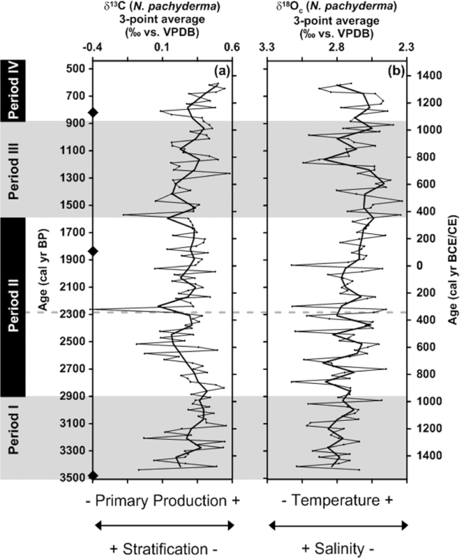
Stable isotope analysis performed on N. pachyderma versus cal. yr BP (left y-axis) and cal. yr BCE/CE (right y-axis). The black diamonds on the y-axis indicate the AMS ¹⁴C converted to calibrated radiocarbon ages. (a) δ¹³C measurements versus age. (b) δ¹⁸O_c measurements corrected for a vital effect of 0.6‰ according to Simstich et al. (2003) and Nyland et al. (2006) versus age.

SST and SSS reconstructions

The SST_Transfer record shows a decrease from 7.2°C to 6.8°C between ca. 3500 and 2900 cal. yr BP (Figures 3h and 6c). At ca. 2900 cal. yr BP, a sharp increase in SST_Transfer is followed by relatively high values (ca. 7.4°C) till ca. 2300 cal. yr BP. Thereafter, the SST_Transfer record decreases reaching a value of ca. 6.8°C at ca. 1600 cal. yr BP. Hereafter, the SST_Transfer record stops its decreasing trend and stabilizes around the value of ca. 6.6°C until ca. 900 cal. yr BP. Eventually, after ca. 900 cal. yr BP, the SST_Transfer record shows a slight decrease towards ca. 6.3°C at the top of the record.

Figure 6.

Reconstructed water mass properties versus cal. yr BP (left y-axis) and cal. yr BCE/CE (right y-axis). The black diamonds on the y-axis indicate the AMS ¹⁴C converted to calibrated radiocarbon ages. (a) Mg/Ca measurements of N. pachyderma versus age. (b) SST_Mg/Ca record obtained by the temperature:Mg/Ca equation of Kozdon et al. (2009) versus age. (c) SST_Transfer record using the modern foraminiferal dataset by Husum and Hald (2012) versus age. (d) SSS record derived by a combined foraminiferal (N. pachyderma) δ¹⁸O_c and SST_Mg/Ca approach using the salinity to δ¹⁸O_w relation by Simstich et al. (2003) versus age. (e) Reconstructed NAO index from a lake record in south-west Greenland (Olsen et al., 2012) versus age.

Between ca. 3500 and 3300 cal. yr BP, the SST_Mg/Ca values show a small decrease from 3.1°C to 2.7°C followed by relatively stable values of ca. 3.3°C until ca. 2900 cal. yr BP (Figure 6b). Furthermore, between ca. 2900 and 2500 cal. yr BP, the SST_Mg/Ca values show a gradual increase from ca. 3.0°C to 4.2°C which are followed by relatively stable values (ca. 3.5°C) between ca. 2100 and 1600 cal. yr BP. Then, around ca. 1600 cal. yr BP, the SST_Mg/Ca record shows an initial decrease towards 2.7°C at ca. 1500 cal. yr BP, whereafter lower values of ca. 3.2°C are recorded, albeit with one exception of a single peak (4.7°C) around ca. 1300 cal. yr BP.

Between ca. 3500 and 2900 cal. yr BP, the reconstructed SSS record shows a gradual decrease from ca. 34‰ to 32‰ (Figure 6d). After ca. 2900 cal. yr BP, the SSS values increase to 34‰ at ca. 2800 cal. yr BP followed by a decrease until ca. 2500 cal. yr BP. Between ca. 2100 and 1600 cal. yr BP, the palaeo SSS record is stable around ca. 33‰, showing the highest values of the record (i.e. 34.0‰). At ca. 1600 cal. yr BP, the SSS record drops, whereafter it continues with lower and stable values (ca. 32‰) till ca. 900 cal. yr BP.

Palaeoceanographic evolution of the late-Holocene

Throughout the late-Holocene, the current proxy records show an overall cooling, for example, the SST_Transfer values decrease from 7.7°C to 6.3°C (Figures 3h and 6c). This general trend is associated with an overall decreased influence of Atlantic water corresponding well to similar observations in the Nordic Seas (e.g. Hald et al., 2007; Skirbekk et al., 2010; Slubowska et al., 2005). This also corresponds to north-western Europe lake and tree records arguing for a late-Holocene trend towards colder and dryer conditions (e.g. Bjune et al., 2009; Kaufman et al., 2009). Nonetheless, at the Vøring plateau south of the study site, planktic foraminiferal data show an overall increased influence of Atlantic water throughout this time period (Andersson et al., 2003, 2010; Risebrobakken et al., 2003). In addition to the overall cooling, the various proxy records within the current study also argue for subtle changes within the oceanographic conditions on a centennial temporal resolution throughout the late-Holocene. These fluctuations of the sub-surface water masses will be further discussed for four separate time periods. Nonetheless, the strict ages of the boundaries as well as the following interpretation should be taken with some caution because of the internal variability within the different periods. But, in order to place the record within a geographically broader context, it is compared with the existing palaeorecords and discussed in terms of possible linkages to NAO conditions. The here interpreted fluctuating influence of sub-surface water masses and their potential link with NAO conditions is presented as schematic profiles across the northern Norwegian margin (Figure 7).

Figure 7.

The interpretation of fluctuating influence of sub-surface water masses based on multi-proxy data from the study area (W00-SC3) is presented as a schematic profile across the northern Norwegian margin (West (W) - East (E) transect) for four separate time periods: Coastal water (CW), Atlantic water (AW), Atlantic intermediate water (AIW), Deep water (DW), positive and negative North Atlantic Oscillation (NAO+ and NAO-).

Period I: ca. 3500–2900 cal. yr BP

Between ca. 3500 and 2900 cal. yr BP, the relative planktic foraminiferal abundances show increased values of G. uvula (ca. 5–20%) and high values (ca. 28–36%) of T. quinqueloba (Figure 3g and d). The latter has been associated with subpolar conditions and Atlantic water (Bé and Tolderlund, 1971; Volkmann, 2000); however, it has also considered to respond rapidly to changes in nutrient supply (Johannessen et al., 1994; Reynolds and Thunnel, 1985). G. uvula has been associated with reduced salinities and Coastal water (Husum and Hald, 2012) as well as with high food supplies and cold productive surface waters (e.g. Bergami et al., 2009; Boltovskoy et al., 1996; Saito et al., 1981). Hence, the high relative abundances of both species strongly argue for an increased influence of colder and less saline Coastal water accompanied with a strong influence of a productive oceanographic front between Coastal and Atlantic water. In addition, both the increasing TOC and δ¹³C values further argue for increased primary production corresponding to an increased influence of an oceanographic front (Figures 4c and 5b).

In contrast, the relatively low planktic foraminiferal concentrations and fluxes, as well as the in general low TOC values, seem to indicate a rather low primary production (Figure 4c and e). However, these values most likely result from the relatively poor preservation conditions as indicated by the generally high planktic foraminiferal fragmentation and the low CaCO₃ values (<22 wt. %; Figure 4a and d). Nonetheless, the mean shell weight results actually show the highest values of the record, but this represents in all likelihood an artefact of the poor preservation conditions. Due to the increased calcite dissolution, smaller species break more likely into fragments and thereby attribute to a skewed sampling in this period with fewer available specimens. And thus, despite the use of a narrow size range, the remaining larger specimens might have led to the highest observed values of the record. Furthermore, as the solubility of CaCO₃ increases with decreasing temperatures (Edmond and Gieskes, 1970), the here recorded low CaCO₃ values argue for an increased influence of colder Coastal water associated with enhanced dissolution conditions. Additionally, these low CaCO₃ values might reflect the dilution by terrigenous material and thereby support the interpretation of enhanced carbonate dissolution at the continental margin off Norway (Huber et al., 2000). However, the latter interpretation should be taken with caution as our age model does not allow a detailed investigation of the sedimentation rate variability.

The depleting δ¹⁸O_c trend can indicate an increased temperature and/or a decreased salinity signal (Figure 5b). Furthermore, the planktic foraminiferal fauna data and decreasing SST_Transfer values from 7.2°C to 6.8°C (Figures 3h and 6c) strongly argue for less saline water masses associated with an increased influence of Coastal water, here most likely, reflected by the δ¹⁸O_c record. Correspondingly, the reconstructed SSS record confirms the overall trend towards less saline conditions (Figure 6d). Nonetheless, contrary to decreasing SST_Transfer values, the overall lower SST_Mg/Ca values remain somehow stable throughout this period (Figure 6c and b). The latter might illustrate the different water depths and/or season that the two proxies represent possibly arguing for more stratified water masses (Berben, 2014).

Overall, the multi-proxy data argue for an increased influence of relative cold and fresh Coastal water and possibly more stratified water masses at the core site. This might be related to a dominating negative NAO-like mode throughout this time interval causing a more westwards located thinning wedge of Coastal water above Atlantic water at the study site (Figure 7a). A 5200-year NAO index has been reconstructed using a multi-proxy geochemical record from a lake in south-west Greenland (Olsen et al., 2012). Although this NAO index generally shows mainly positive values, a stronger influence of negative NAO conditions has been identified between ca. 4500 and 2500 cal. yr BP which possibly correspond to the here suggested negative NAO-like conditions (Figure 6e). In addition to this, the reconstruction of past atmospheric circulation variability, based on exotic pollen analysis of marine sediments from Newfoundland, illustrated a major shift from dominantly zonal (linked to a positive NAO) to a more meridional (associated with a negative NAO regime) atmospheric circulation pattern at ca. 3000 cal. yr BP (Jessen et al., 2011). The latter are generally associated with a reduced inflow of Atlantic water and a stronger influence of Coastal water (e.g. Hurrell et al., 2013; Sætre, 2007). Correspondingly, between ca. 3500 and 2500 cal. yr BP, the reconstructed SST record from the Vøring plateau (66.58°N, 07.38°E) shows decreasing values arguing for a reduced influence of Atlantic water (Andersson et al., 2003, 2010; Risebrobakken et al., 2003). Furthermore, negative NAO conditions resulted in a colder and dryer climate in north-western Europe (e.g. Wanner et al., 2001). A decreasing temperature and precipitation trend throughout this time interval was observed by pollen and plant macrofossil analyses from a lake record in northern Norway (66.25°N, 14.03°E; Bjune and Birks, 2008). Based on the mean ablation-season temperature and winter snow accumulation, a decreased winter precipitation was also observed between 3500 and 3200 cal. yr BP in western Norway (Nesje et al., 2001). Furthermore, surface ground temperatures were reconstructed by applying the speleothem delta function to a measured δ¹⁸O speleothem record from northern Norway which also showed decreased values throughout this time interval (Lauritzen and Lundberg, 1999).

Period II: ca. 2900–1600 cal. yr BP

After ca. 2900 cal. yr BP, a change in the planktic foraminifera’s faunal distribution has been recorded. Between ca. 2900 and 1600 cal. yr BP, the latter is characterized by high relative abundances of N. incompta, T. quinqueloba, G. glutinata and G. bulloides (Figure 3c–f). These species have all been associated with subpolar conditions and warm Atlantic surface water masses (e.g. Bé and Tolderlund, 1971; Carstens et al., 1997; Johannessen et al., 1994; Simstich et al., 2003) and thus argue for a pronounced influence of Atlantic water brought to the study area by the NwAC.

Overall, the total planktic foraminiferal concentration and flux values show higher and increasing values, especially between ca. 2300 and 1600 cal. yr BP, possibly indicative of increased primary production (Figures 3a and 4e). However, at ca. 2900 cal. yr BP, the δ¹³C record shows a clear shift towards depleted values at ca. 2300 cal. yr BP (Figure 5a). Thereafter, the δ¹³C values remain relatively stable (ca. 0.3‰) and thus argue for less primary production throughout this period. The seemingly increased primary production as reflected by higher flux and concentration likely results from the generally improved preservation conditions. The slightly reduced fragmentation and increasing CaCO₃ values (up to ca. 30 wt. %) argue for a gradual trend towards reduced dissolution conditions throughout this period (Figure 4a and d). More favourable preservation conditions have previously been associated with increased influence of Atlantic surface water where pore waters are supersaturated with respect to calcium because of the lower organic matter productivity and a higher rain of CaCO₃ (e.g. Henrich et al., 2002; Huber et al., 2000).

The δ¹⁸O_c record continues its depleting trend from period I possibly reflecting an increased temperature and/or reduced salinity signal (Figure 5b). The planktic foraminiferal fauna data and the clearly elevated SST_Transfer values (ca. 7.4°C) after ca. 2900 cal. yr BP argue for increasing temperatures which are most likely related to an increased influence of Atlantic water (Figures 3h and 6c). Correspondingly, the palaeo SSS record shows overall higher values up to ca. 34‰ and thus correlates to an increased influence of more saline Atlantic water (Figure 6d). In addition, the SST_Mg/Ca record starts an increasing trend at ca. 2900 cal. yr BP followed by higher values (ca. 0.5–1.0°C higher than during period I) and thus could also be linked to an increased influence of Atlantic water (Figure 6b).

The here recorded increased influence of Atlantic water might be caused because of the positive NAO conditions which are associated with stronger westerlies across the North Atlantic (e.g. Hurrell et al., 2013). A close correlation between the NAO and the longitudinal (east-west) extents of Atlantic water in the NwAC has previously been observed (Blindheim et al., 2000). Positive NAO conditions result in a narrowing of the NwAC and thereby an enhanced influence of Atlantic water pushed closer towards the Norwegian margin. This possibly reduced the influence of Coastal water at the study area leading to a more eastwards located thinning wedge of Coastal water above Atlantic water (Figure 7b). Throughout this time period, Olsen et al. (2012) observed a general increasing trend in their NAO index which might correspond to the here interpreted influence of a positive NAO mode (Figure 6e). Similarly, high SSTs associated with a strengthened inflow of Atlantic water have also been observed at the Vøring plateau between ca. 2500 and 1600 cal. yr BP (Andersson et al., 2003, 2010; Risebrobakken et al., 2003). Additionally, increased temperatures in northern Norway have been observed throughout this time interval from a lake record (Bjune and Birks, 2008) and a speleothem record (Lauritzen and Lundberg, 1999). Furthermore, between ca. 2700 and 1900 cal. yr BP, increased winter precipitation has been observed in western Norway (Nesje et al., 2001). These observations correlate well to the warmer and wetter climate scenarios attributed to positive NAO conditions in north-western Europe (e.g. Wanner et al., 2001).

Although the following interpretation might require a better age constrain on some of the here recorded main events, the last part of period II could be corresponding to the RWP observed between ca. 2000 and 1550 cal. yr BP (ca. BCE 50–CE 400; Lamb, 1977). A period of warmer temperatures in northern Norway has also been linked to the RWP by Lauritzen and Lundberg (1999). Contrary to the relative warm RWP conditions in north-western Europe (e.g. Lamb, 1977), benthic foraminiferal and diatom data showed increased seasonal sea ice formation and reduced influence of Atlantic water between 2700 and 1600 cal. yr BP in the Labrador Sea, south-west Greenland (Seidenkrantz et al., 2007). A general decreased influence of Atlantic water was also indicated by IC strength proxies on the southeast Greenland shelf between ca. 3600 and 1500 cal. yr BP (Andresen et al., 2012). During a positive NAO mode, the subpolar gyre circulation is stronger and more east-west oriented, resulting in a reduced influence of the IC south of Greenland (Hatun et al., 2005; Sarafanov, 2009). Furthermore, this opposite signal of a reduced Atlantic water component in the eastern part of the North Atlantic Ocean was suggested to result in a so-called Atlantic oceanographic see-saw pattern in the climatic response to NAO changes (Seidenkrantz et al., 2007). This see-saw pattern of anomalously high ocean temperatures in the eastern versus anomalously low in the western parts of the North Atlantic Ocean during a positive NAO corresponds to a previous study on modern conditions by Wanner et al. (2001).

Period III: ca. 1600–900 cal. yr BP

At ca. 1600 cal. yr BP, the highest recorded values of both the planktic foraminiferal concentration and flux were followed by a sharp transition to low values (Figures 3a and 4e). The latter remained stable until ca. 900 cal. yr BP. Further during this time interval, the planktic foraminiferal fauna shows more stable values for all species with particularly high values of G. uvula (ca. 15–27%; Figure 3g) which tolerates somewhat lowered salinities (e.g. Husum and Hald, 2012). These results likely reflect a stable period with a strong influence of Coastal water. Simultaneously, at ca. 1600 cal. yr BP, the CaCO₃ record shifts towards an overall decreasing trend and the mean shell weight shows somewhat reduced values compared with period II (Figure 4d and b). This could indicate slightly reduced preservation conditions, possibly related to an enhanced influence of Coastal water and dilution of terrigenous material (e.g. Huber et al., 2000). Correspondingly, the δ¹³C record increases after ca. 1600 cal. yr BP which indicates enhanced primary production conditions and thereby argues for a returned influence of Coastal water causing productive conditions near a stronger oceanic front (Figure 5a).

Although δ¹⁸O_c values initially continue their decreasing trend towards ca. 1300 cal. yr BP, they eventually increase and thereby argue for a possible reduction in temperature (Figure 5b). All reconstructed water mass properties show at ca. 1600 cal. yr BP a transition towards stable and lower values (Figure 6b–d). Both the SST_Transfer (ca. 6.6°C) and SST_Mg/Ca records show lower values, down to 1.0°C less than the previous period II, hence indicating a reduced influence of relatively warm Atlantic water (Figure 6c and b). The SSS record, in particular, shows a well-pronounced rapid decrease at ca. 1600 cal. yr BP, and compared with period II, ca. 0.5–1.0‰ lower values. Hence, it also argues for a reduced influence of Atlantic water or an enhanced influence of Coastal water (Figure 6d).

The multi-proxy data arguing for a shift towards a strong influence of Coastal water is further interpreted as a westwards migrated thinning wedge of Coastal water which might be associated with a change towards negative NAO conditions (e.g. Sætre, 2007; Figure 7c). Within this time interval, the current multi-proxy record corresponds well to other marine and terrestrial palaeorecords from the region. SST records from the Vøring plateau have shown a sharp decrease at ca. 1600 cal. yr BP, whereas the values remained relatively low and stable compared with the previous period (Andersson et al., 2003, 2010; Risebrobakken et al., 2003). This also suggests a reduced influence of Atlantic water towards the core site. Furthermore, a colder and dryer climate associated with the DA was suggested by low surface ground temperatures between ca. 1500 and 900 cal. yr BP in northern Norway (e.g. Lauritzen and Lundberg, 1999). Furthermore, Bjune and Birks (2008) also observed decreasing air temperatures between ca. 1800 and 800 cal. yr BP in northern Norway.

The here carefully suggested negative NAO conditions and its associated colder and dryer climate in north-western Europe do, however, not correlate with the overall positive NAO mode reconstructed by Olsen et al. (2012) during this time interval (Figure 6e). Nonetheless, similar to period II, Seidenkrantz et al. (2007) observed an opposite pattern of Atlantic water inflow contradictive with the deteriorate climate in north-western Europe. In particular, their benthic foraminiferal record has been indicating an increased influx of saline water brought to the Labrador Sea by the WGC between 1600 and 1200 cal. yr BP. These contradictory observations are attributed to the previously mentioned Atlantic oceanographic see-saw pattern whereby an opposite signal of ocean temperatures between the eastern and western North Atlantic Ocean has been attributed to the dominating NAO mode (Wanner et al., 2001). Such a link between SST anomalies in the subpolar gyre to a negative NAO and cold winters in north-west Europe has also been made in previous studies (Luterbacher et al., 2002; Miettinen et al., 2011). Based on fossil diatom assemblages from the northern subpolar North Atlantic, a close link between NAO fluctuations and the strength variability of the eastern and western branches of the NwAC has been indicated (Miettinen et al., 2011, 2012). During a negative NAO mode, weakened westerly winds over the Atlantic result in profoundly increased influence of warm Atlantic water flowing westwards by the IC (Miettinen et al., 2011, 2012). This close coupling between ocean and atmosphere supports the here interpreted negative NAO conditions throughout this period (Figure 7c).

Period IV: ca. 900–550 cal. yr BP

The clearly decreasing values in the relative abundance of G. uvula after ca. 900 cal. yr BP indicate a decreased influence of Coastal water (Figure 3g). The concomitant increase in N. incompta correspondingly suggests a stronger influence of subpolar conditions and thus a stronger influence of Atlantic water (e.g. Bé and Tolderlund, 1971; Figure 3c). Nonetheless, the increased abundance of N. pachyderma argues for increased polar conditions (e.g. Bé and Tolderlund, 1971; Volkmann, 2000; Figure 3b) which is reflected by the reduced SST_Transfer record reaching the lowest value (6.3°C) of this study around ca. 550 cal. yr BP (Figures 3h and 6c). Previously, proxy data from a Greenland ice core, used to reconstruct changes in atmospheric circulation patterns, indicated a shift at ca. 550 cal. yr BP (ca. AD 1400) towards low sea level pressure associated with decreased SST in the North Atlantic (Meeker and Mayewski, 2002), which correlates well to the here observed reduced SST_Transfer values. Furthermore, a gently increased abundance of N. pachyderma was also found throughout the last ca. 1000 cal. yr BP at the Vøring plateau (Risebrobakken et al., 2003). However, regardless of this similarity, the SST reconstructions from the Vøring plateau show increasing values during this time interval (Andersson et al., 2003, 2010; Risebrobakken et al., 2003). The contradictory results of these records are most likely because of the use of different transfer functions. The transfer function based on the >100 µm modern analogue dataset used in this study has previously indicated to result in generally lower temperatures (Husum and Hald, 2012). Furthermore, the potential influence of selective dissolution (e.g. Berger, 1970; Le and Thunell, 1996; Thunell and Honjo, 1981) might have altered the foraminiferal assemblage composition, resulting in an enrichment of the most dissolution-resistant thick-shelled species N. pachyderma (e.g. Hemleben et al., 1989; Metzler et al., 1982). Additionally, the SST_Transfer record in this study has been reconstructed for a water depth of 100 m, whereas the SST record of the Vøring plateau reflects temperatures at a 10-m water depth. These different represented water depths, however, seem to mainly explain the overall lower SST values in this study, rather than explaining the differences in trends (Husum and Hald, 2012). Wind-induced mixing of the surface layer is most likely responsible for the warmer temperatures at 10 m water depth. Finally, the generally colder SST_Transfer values are most likely because of the overall cooling trend observed throughout the record and linked to decreasing solar insolation values throughout the late-Holocene (e.g. Hald et al., 2007; Kaufman et al., 2009).

After ca. 900 cal. yr BP, the planktic foraminiferal concentrations and fluxes slightly decrease which might indicate reduced primary production (Figures 3a and 4e). The TOC record stabilizes after ca. 900cal. yr BP around somewhat lower values compared with the end of period III which might indicate a small reduction in primary production. The latter likely reflects a small shift away from productive oceanic front conditions. At ca. 900 cal. yr BP, both the fragmentation and mean shell weight records show a pronounced increase (Figure 4a and b). The increased fragmentation argues for deteriorated preservation conditions in the sediment, whereas the increased shell weight indicates reduced dissolution of calcite. These conflicting interpretations might be best explained by the different representation of these dissolution proxies and/or the different influences affecting the results. The shell weight reflects the dissolution caused by mass loss in an adult stage of N. pachyderma, whereas the fragmentation represents fragments of all species including those of juvenile forms of N. pachyderma. Furthermore, environmental conditions such as nutrient availability, temperature and/or salinity can affect the final shell weight during growth (e.g. Barker and Elderfield, 2002). The fragmentation results could be affected by mechanical destruction during sieving which might create an increased amount of fragments. Nonetheless, the relatively high and stable CaCO₃ values, recorded after ca. 900 cal. yr BP, are indicative of reduced dissolution conditions (Figure 4d). The latter is associated with conditions marked by an increased influence of Atlantic water (Huber et al., 2000). The increasing δ¹³C record might further indicate a reduced stratification at the core site resulting from an increased influence of Atlantic water (Figure 5a).

Despite the overall cooling trend, several of the here presented proxies do argue for changing oceanographic conditions after ca. 900 cal. yr BP. In this study, the interpreted returned influence of Atlantic water might be the result of generally positive NAO conditions (Figure 7d). The reconstructed NAO index from south-west Greenland also indicates positive NAO conditions during this time interval which are associated with the MWP (Olsen et al., 2012; Figure 6e). Furthermore, this also corresponds to the results of a NAO reconstruction based on tree rings and speleothems that indicate a dominating positive NAO mode associated with an intensified AMOC (Trouet et al., 2009). These conditions are expressed by a reduced influence of Coastal water and a stronger moisture and heat transport to Norway by the NwAC resulting in warmer and wetter climatic conditions (e.g. Hurrell et al., 2013; Wanner et al., 2001). This correlates well to terrestrial records from northern Norway which show slightly increasing air temperatures for this time interval (Bjune and Birks, 2008) and high surface ground temperatures between ca. 800 and 500 cal. yr BP (Lauritzen and Lundberg, 1999). Hence, this time interval possibly reflects the warmer conditions associated with the MWP which correlates with observation at the Vøring plateau between ca. 1150 and 650 cal. yr BP (ca. AD 800–1300; Nyland et al., 2006) and in northern Norway between ca. 800 and 500 cal. yr BP (ca. AD 1150–1450; Lauritzen and Lundberg, 1999). Between 1200 and 800 cal. yr BP, a returned seasonal sea ice cover presumably related to relatively cold climatic conditions (relatively similar to the RWP) has been observed in the Labrador Sea with Atlantic water only entering as a weak sub-surface current (Seidenkrantz et al., 2007). These observations correlate well to the aforementioned oceanographic see-saw pattern resulting from positive NAO conditions (Miettinen et al., 2011, 2012; Wanner et al., 2001).

Conclusion

A marine core from the northern Norwegian margin was investigated to elucidate the natural variability of water mass properties throughout the late-Holocene on a centennial temporal resolution. In this study, a multi-proxy approach of palaeo SST and SSS data illustrated the palaeoceanographic evolution of the late-Holocene. The latter was discussed in terms of changing influences of Atlantic and Coastal water. Because of the internal variability within the four different periods, the suggested linkages to fluctuating modes of the NAO should be taken with caution. Nonetheless, the multi-proxy data allow for a broad interpretation and are therefore placed into a geographically wider context.

Overall, the proxy results indicate a general cooling trend throughout the late-Holocene from ca. 8°C to 6°C (SST_Transfer). In addition, subtle fluctuating conditions of Atlantic and Coastal water intensity are observed during this time interval. Period I (ca. 3500–2900 cal. yr BP) is influenced by relatively cold (ca. 6.8°C, SST_Transfer) and less saline Coastal water and a stronger vertical stratification of the water column. These conditions might be linked to dominating negative NAO-like conditions. Throughout period II (ca. 2900–1600 cal. yr BP), the core site experiences a stronger influence of warm Atlantic water (ca. 7.4°C, SST_Transfer) with more favourable preservation conditions possibly related to positive NAO conditions. The last part of this period might correspond to the RWP in north-western Europe. Stable conditions and cold SSTs (ca. 6.6°C, SST_Transfer) are observed within period III (ca. 1600–900 cal. yr BP) indicating a returned and stronger influence of Coastal water. The conditions during this period are in this study attributed to a negative NAO mode and potentially correspond to the colder and dryer DA. Period IV (ca. 900–550 cal. yr BP) shows a returned and stronger influence of Atlantic water which could be associated with dominating positive NAO conditions and the MWP. Nonetheless, Atlantic water reaching the core site was less warm (ca. 6.3°C, SST_Transfer) compared with period II because of the overall late-Holocene cooling. In addition, when comparing the results with previously published records, they indicated an opposite climatic response to changing NAO modes between the eastern and western North Atlantic Ocean and thereby a close coupling between ocean and atmosphere within the climate system.

Footnotes

Acknowledgements

Jan Sverre Laberg is acknowledged for providing the marine sediment core and Jochen Knies for access to the TOC and CaCO₃ data. Additionally, thanks are also extended to Jan P. Holm for his help in preparing the maps and Trine Dahl, Julia Sen and Karina Monsen for assisting with laboratory work at UiT – The Arctic University of Norway. Further, thanks to two anonymous referees who provided helpful and informative reviews. All new data, presented within this paper, can be found within the supporting information file (available online).

Funding

This work was carried out within the framework of the Initial Training Network programme ‘Changing Arctic and Subarctic Environments’ (CASE, grant agreement no. 238111) funded by the European Commission within the 7th Framework Program People, the Research Council of Norway, in addition to UiT – The Arctic University of Norway and the Norwegian Polar Institute.

References

Andersson

Pausata

FSR

Jansen

. (2010) Holocene trends in the foraminifer record from the Norwegian Sea and the North Atlantic Ocean. Climate of the Past 6: 179–193.

Andersson

Risebrobakken

Jansen

. (2003) Late-Holocene surface ocean conditions of the Norwegian Sea (Voring Plateau). Paleoceanography 18: PA1044.

Andresen

Hansen

Seidenkrantz

. (2012) Mid- to late-Holocene oceanographic variability on the Southeast Greenland shelf. The Holocene 23(2): 167–178.

Aspeli

(1994) Late Quaternary benthic foraminiferal stratigraphy on the western Barents slope Sea. Unpublished Thesis, University of Tromsø (in Norwegian).

Barker

Elderfield

(2002) Foraminiferal calcification response to glacial interglacial changes in atmospheric CO₂. Science 297: 833–836.

Barker

Kiefer

Elderfield

(2004) Temporal changes in North Atlantic circulation constrained by planktonic foraminiferal shell weights. Paleoceanography 19: PA3008.

Bé

AWH

Tolderlund

(1971) Distribution and ecology of living planktonic foraminifera in surface waters of the Atlantic and Indian Oceans. In: Funnell

Riedel

(eds) The Micropaleontology of the Oceans. London: Cambridge University Press, pp. 105–149.

Beer

Schiebel

Wilson

(2010) Testing planktic foraminiferal shell weight as a surface water [CO₃^2-] proxy using plankton net samples. Geology 38: 103–106.

Berben

SMP

(2014) A Holocene palaeoceanographic multi-proxy study on the variability of Atlantic water inflow and sea ice distribution along the pathway of Atlantic water. PhD Thesis, University of Tromsø.

10.

Berben

SMP

Husum

Cabedo-Sanz

. (2014) Holocene sub-centennial evolution of Atlantic water inflow and sea ice distribution in the western Barents Sea. Climate of the Past 10: 181–198.

11.

Bergami

Capotondi

Langone

. (2009) Distribution of living planktonic foraminifera in the Ross Sea and the Pacific sector of the Southern Ocean (Antarctica). Marine Micropaleontology 73: 37–48.

12.

Berger

(1970) Planktonic foraminifera: Selective solution and the Lysocline. Marine Geology 8: 111–138.

13.

Bjune

Birks

HJB

(2008) Holocene vegetation dynamics and inferred climate changes at Svanåvatnet, Mo i Rana, northern Norway. Boreas 37: 146–156.

14.

Bjune

Seppä

Birks

HJB

(2009) Quantitative summer temperature reconstructions for the last 2000 years based on pollen-stratigraphical data from northern Fennoscandia. Journal of Paleolimnology 41: 43–56.

15.

Blindheim

Borovkov

Hansen

. (2000) Upper layer cooling and freshening in the Norwegian Sea in relation to atmospheric forcing. Deep Sea Research Part I 47: 655–680.

16.

Boltovskoy

Correa

. (1996) Planktic foraminifera from the southwestern Atlantic (30°–60°S): Species-specific patterns in the upper 50 m. Marine Micropaleontology 28: 53–72.

17.

Broecker

Clark

(2001) An evaluation of Lohmann’s foraminifera weight dissolution index. Paleoceanography 16: 531–534.

18.

Bryson

Goodman

(1980) Volcanic activity and climate change. Science 207: 1041–1044.

19.

Carstens

Hebbeln

Wefer

(1997) Distribution of planktic foraminifera at the ice margin in the Arctic (Fram Strait). Marine Micropaleontology 29: 257–269.

20.

Cifelli

(1961) Globigerina incompta, a new species of pelagic foraminifera from the North Atlantic. Contributions Cushman Foundation Foraminiferal Research 12: 83–86.

21.

Conan

SMH

Ivanova

Brummer

GJA

(2002) Quantifying carbonate dissolution and calibration of foraminiferal dissolution indices in the Somali Basin. Marine Geology 182: 325–349.

22.

Darling

Kucera

Kroon

. (2006) A resolution for the coiling direction paradox in Neogloboquadrina pachyderma. Paleoceanography 21: PA2011.

23.

Duplessy

Ivanova

Murdmaa

. (2001) Holocene paleoceanography of the northern Barents Sea and variations of the northward heat transport by the Atlantic Ocean. Boreas 30: 2–16.

24.

Edmond

Gieskes

(1970) On the calculation of the degree of saturation of sea water with respect to calcium carbonate under in situ conditions. Geochimica et Cosmochimica Acta 35: 1261–1291.

25.

Ehrmann

Thiede

(1985) History of Mesozoic and Cenozoic sediment fluxes to the North Atlantic Ocean. In: Füchtbauer

Lisitzyn

Milliman

(eds) Contributions to Sedimentology, no. 15. Stuttgart: E. Schweizerbart’sche Verlagsbuchhandlung, pp. 1–109.

26.

Elderfield

Ganssen

(2000) Past temperature and delta ¹⁸O of surface ocean waters inferred from foraminiferal Mg/Ca ratios. Nature 405: 442–445.

27.

Elderfield

Greaves

Barker

. (2010) A record of bottom water temperature and seawater [delta]¹⁸O for the Southern Ocean over the past 440 kyr based on Mg/Ca of benthic foraminiferal Uvigerina spp. Quaternary Science Reviews 29: 160–169.

28.

Espitalié

Laporte

Madec

. (1977) Méthode rapide de characterisation des roches-mere, de leur potential petrolier et de leur degre d’évolution. Revue de l’Institute Francais du Petrole 32: 23–42.

29.

Giraudeau

Jennings

Andrews

(2004) Timing and mechanisms of surface and intermediate water circulation changes in the Nordic seas over the last 10,000 cal years: A view from the north Iceland shelf. Quaternary Science Reviews 23: 2127–2139.

30.

Hald

Andersson

Ebbesen

. (2007) Variations in temperature and extent of Atlantic water in the northern North Atlantic during the Holocene. Quaternary Science Reviews 26: 3423–3440.

31.

Hatun

Sand

Drange

. (2005) Influence of the Atlantic Subpolar Gyre on the thermohaline circulation. Science 309: 1841–1844.

32.

Hemleben

Spindler

Anderson

(1989) Modern Planktonic Foraminifera. New York: Springer-Verlag, p. 363.

33.

Henrich

Baumann

Huber

. (2002) Carbonate preservation records of the past 3 Myr in the Norwegian-Greenland Sea and the northern North Atlantic: Implications for the history of NADW production. Marine Geology 184: 17–39.

34.

Hopkins

(1991) The GIN Sea: A synthesis of its physical oceanography and literature review, 1972–1985. Earth-Science Reviews 30: 175–318.

35.

Huber

Meggers

Baumann

. (2000) Recent and Pleistocene carbonate dissolution in sediments of the Norwegian-Greenland Sea. Marine Geology 165: 123–136.

36.

Hurdle

(1986) The Nordic Seas. New York: Springer.

37.

Hurrell

Kushnir

Ottersen

. (2013) An overview of the North Atlantic Oscillation. In: Hurrell

Kushnir

Ottersen

. (eds) The North Atlantic Oscillation: Climatic Significance and Environmental Impact. Washington, DC: American Geophysical Union, pp. 1–35.

38.

Husum

Hald

(2012) Arctic planktic foraminiferal assemblages: Implications for subsurface temperature reconstructions. Marine Micropaleontology 96(97): 38–47.

39.

Ikeda

Johannessen

Lygre

. (1989) A process study of mesoscale meanders and eddies in the Norwegian Coastal Current. Journal of Physical Oceanography 19: 20–35.

40.

Jernas

Klitgaard Kristensen

Husum

. (2013) Palaeoenvironmental changes of the last two millennia on the western and northern Svalbard shelf. Boreas 42: 236–255.

41.

Jessen

Solignac

Nørgaard-Pedersen

. (2011) Exotic pollen as an indicator of variable atmospheric circulation over the Labrador Sea region during the mid-to late-Holocene. Journal of Quaternary Science 26(3): 286–296.

42.

Jiang

Eiriksson

Schulz

. (2005) Evidence for solar forcing of sea-surface temperature on the North Icelandic Shelf during the Late-Holocene. Geology 33(1): 73–76.

43.

Johannessen

Jansen

Flatøy

. (1994) The relationship between surface water masses, oceanographic fronts and plaeoclimatic proxies in surface sediments of the Greenland, Iceland, Norwegian Seas. In: Zahn

Pedersen

Kaminski

. (eds) Carbon Cycling in the Glacial Ocean: Constraints of the Ocean’s Role in Global Change. Berlin: Springer, pp. 61–86.

44.

Katz

Cramer

Franzese

. (2010) Traditional and emerging geochemical proxies in foraminifera. Journal of Foraminiferal Research 40(2): 165–192.

45.

Kaufman

Schneider

McKay

. (2009) Recent warming reverses long-term Arctic cooling. Science 325: 1236–1239.

46.

Knudsen

(1998) Foraminiferer i Kvartær stratigrafi: Laboratorie og fremstillingsteknik samt udvalgte eksempler. Geologisk Tidsskrift 3: 1–25.

47.

Kozdon

Eisenhauer

Weinelt

. (2009) Reassessing Mg/Ca temperature calibrations of Neogloboquadrina pachyderma (sinistral) using paired d44/40Ca and Mg/Ca measurements. Geochemistry, Geophysics, Geosystems 10: Q03005.

48.

Laberg

Vorren

Mienert

. (2002) The Trænadjupet slide: A large slope failure affecting the continental margin of Norway 4,000 years ago. Geo-Marine Letters 22: 19–24.

49.

Lamb

(1977) Climate, Present, Past and Future. Volume 2: Climatic History and the Future. London: Methuen & Co Ltd, p. 835.

50.

Lauritzen

Lundberg

(1999) Calibration of the speleothem delta function: An absolute temperature record for the Holocene in northern Norway. The Holocene 9(6): 650–669.

51.

Thunell

(1996) Modelling planktic foraminiferal assemblages changes and application to sea surface temperature estimation in the western equatorial Pacific Ocean. Marine Micropaleontology 28: 211–229.

52.

Lean

(2002) Solar forcing of climate change in recent millennia. In: Wefer

Berger

Behre

. (eds) Climate Development and History of the North Atlantic Realm. Berlin: Springer-Verlag, pp. 75–88.

53.

Lubinski

Polyak

Forman

(2001) Freshwater and Atlantic water inflows to the deep northern Barents and Kara seas since ca 13 ¹⁴Cka: Foraminifera and stable isotopes. Quaternary Science Reviews 20: 1851–1879.

54.

Luterbacher

Xoplaki

Dietrich

. (2002) Extending North Atlantic Oscillation reconstructions back to 1500. Atmospheric Science Letters 2: 114–124.

55.

Mangerud

Bondevik

Gulliksen

. (2006) Marine ¹⁴C reservoir ages for 19^th century whales and molluscs from the North Atlantic. Quaternary Science Reviews 25: 3228–3245.

56.

Mashiotta

Lea

Spero

(1999) Glacial interglacial changes in Subantarctic sea surface temperature and d¹⁸O-water using foraminiferal Mg. Earth and Planetary Science Letters 170: 417–432.

57.

Meeker

Mayewski

(2002) A 1400-year high-resolution record of atmospheric circulation over the North Atlantic and Asia. The Holocene 12(3): 257–266.

58.

Metzler

Wenkam

Berger

(1982) Dissolution of foraminifera in the Eastern Equatorial Pacific: An in situ experiment. Journal of Foraminiferal Research 12(4): 362–368.

59.

Miettinen

Divine

Koç

. (2012) Multicentennial variability of the sea surface temperature gradient across the subpolar North Atlantic over the last 2.8 kyr. Journal of Climate 25: 4205–4219.

60.

Miettinen

Koç

Hall

. (2011) North Atlantic sea surface temperatures and their relation to the North Atlantic Oscillation during the last 230 years. Climate Dynamics 36: 533–543.

61.

Nesje

Matthews

Dahl

. (2001) Holocene glacier fluctuation of Flatebreen and winter-precipitation changes in the Jostedalsbreen region, western Norway, based on glaciolacustrine sediment records. The Holocene 11: 267–280.

62.

Nyland

Jansen

Elderfield

. (2006) Neogloboquadrina pachyderma (dex. and sin.) Mg/Ca and d¹⁸O records from the Norwegian Sea. Geochemistry, Geophysics, Geosystems 7: Q10P17.

63.

Olsen

Anderson

Knudsen

(2012) Variability of the North Atlantic Oscillation over the past 5200 years. Nature Geoscience 5: 808–812. Available at: ftp://ftp.ncdc.noaa.gov/pub/data/paleo/paleolimnology/greenland/lake-ss1220-2012.xls.

64.

Orvik

Niiler

(2002) Major pathways of Atlantic water in the northern North Atlantic and Nordic Seas toward Arctic. Geophysical Research Letters 29(19): 1896.

65.

Ottersen

Planque

Belgrano

. (2001) Ecological effects of the North Atlantic Oscillation. Oecologia 128: 1–14.

66.

Perkins

Hopkins

Malmberg

. (1998) Oceanographic conditions east of Iceland. Journal of Geophysical Research 103: 21531–21542.

67.

Pufhl

Shackleton

(2004) Two proximal, high-resolution records of foraminiferal fragmentation and their implications for changes in dissolution. Deep Sea Research Part I 51: 809–832.

68.

Rasmussen

Thomsen

(2010) Holocene temperature and salinity variability of the Atlantic Water inflow to the Nordic Seas. The Holocene 20(8): 1223–1234.

69.

Reimer

Bard

Bayliss

. (2013) IntCal13 and Marine13 radiocarbon age calibration curves. Radiocarbon 55(4): 1869–1887.

70.

Reynolds

Thunnel

(1985) Seasonal succession of planktonic foraminifera in the subpolar North Pacific. Journal of Foraminiferal Research 15: 282–301.

71.

Risebrobakken

Jansen

Mjele

. (2003) A high resolution study of Holocene paleoclimatic and paleoceanographic changes in the Nordic Seas. Paleoceanography 18: 1017.

72.

Rørvik

Laberg

Hald

. (2010) Behavior of the northwestern part of the Fennoscandian ice sheet during the Last Glacial Maximum – A response to external forcing. Quaternary Science Reviews 29: 2224–2237.

73.

Sætre

(2007) The Norwegian Coastal Current: Oceanography and Climate. Trondheim: Tapir Academic Press, pp. 89–99.

74.

Saito

Thompson

Breger

(1981) Systematic Index of Recent and Pleistocene Planktonic Foraminifera. Tokyo: University of Tokyo Press, pp. 1–190.

75.

Sarafanov

(2009) On the effect of the North Atlantic Oscillation on temperature and salinity of the subpolar North Atlantic intermediate and deep waters. ICES Journal оf Marine Science 66(7): 1448–1454.

76.

Seidenkrantz

Aagaard-Sørensen

Sulsbrück

. (2007) Hydrography and climate of the last 4400 years in a SW Greenland fjord: Implications for Labrador Sea palaeoceanography. The Holocene 17(3): 387–401.

77.

Simstich

Sarnthein

Erlenkeuser

(2003) Paired δ¹⁸O signals of N. pachyderma (s) and T. quinqueloba show thermal stratification structure in the Nordic seas. Marine Micropaleontology 48: 107–125.

78.

Skirbekk

Klitgaard Kristensen

Rasmussen

. (2010) Holocene Climate Variations at the Entrance to a Warm Arctic Fjord: Evidence from Kongsfjorden Trough, Svalbard. London: Geological Society of London (Special Publications 344), pp. 289–304.

79.

Slubowska

Koç

Rasmussen

. (2005) Changes in the flow of Atlantic water into the Arctic Ocean since the last deglaciation: Evidence from the northern Svalbard continental margin, 80N. Paleoceanography 20: PA4014.

80.

Slubowska-Woldengen

Rasmussen

Koç

. (2007) Advection of Atlantic Water to the western and northern Svalbard shelf since 17 500 cal yr BP. Quaternary Science Reviews 26: 463–478.

81.

Solignac

Giraudeau

De Vernal

(2006) Holocene sea surface conditions in the western North Atlantic: Spatial and temporal heterogeneities. Paleoceanography 21: PA2004.

82.

Spielhagen

Erlenkeuser

(1994) Stable oxygen and carbon isotopes in planktic foraminifera from the Arctic Ocean surface sediments: Reflection of the low salinity surface water layer. Marine Geology 119: 227–250.

83.

Stuiver

Reimer

(1993) Extended 14C data base and revised CALIB 3.0 ¹⁴C age calibration program. Radiocarbon 35: 215–230.

84.

Thornalley

DJR

Elderfield

McCave

(2009) Holocene oscillations in temperature and salinity of the surface subpolar North Atlantic. Nature 457: 711–714.

85.

Thunell

Honjo

(1981) Calcite dissolution and the modification of planktonic foraminiferal assemblages. Marine Micropaleontology 6: 169–182.

86.

Trouet

Esper

Graham

. (2009) Persistent positive North Atlantic Oscillation mode dominated the Medieval Climate Anomaly. Science 324: 78–80.

87.

Vellinga

Wood

(2002) Global climatic impacts of a collapse of the Atlantic thermohaline circulation. Climate Change 54: 251–267.

88.

Volkmann

(2000) Planktic foraminifers in the outer Laptev Sea and the Fram Strait: Modern distribution and ecology. Journal of Foraminiferal Research 30: 157–176.

89.

Wanner

Beer

Bütikofer

. (2008) Mid- to Late-Holocene climate change: An overview. Quaternary Science Reviews 27(19–20): 1–38.

90.

Wanner

Brönnimann

Casty

. (2001) North Atlantic Oscillation – Concepts and studies. Surveys in Geophysics 22: 321–381.

91.

Werner

Spielhagen

Bauch

. (2013) Atlantic Water advection versus sea-ice advances in the eastern Fram Strait during the last 9 ka: Multiproxy evidence for a two-phase Holocene. Paleoceanography 28: 283–295.

92.

Zamelczyk

Rasmussen

Husum

. (2013) Marine calcium carbonate preservation vs. climate change over the last two millennia in the Fram Strait: Implications for planktic foraminiferal paleostudies. Marine Micropaleontology 98: 14–27.