
Abstract
In order to improve the reliability of climate models in their projections for the future, spatially and temporally detailed paleoclimate proxy data are needed. In this study, we examined annually laminated sediments from Lake Nurmijärvi (Finland) for their fossil Chironomidae assemblages over a time period with available meteorological observational data (since 1830s). In doing so, we correlated chironomid-based inferences of summer air temperatures against instrumentally measured values using two different reconstruction approaches, namely, calibration-in-space (CiS, multilake training set) and calibration-in-time (CiT, calibration of time series data against meteorological data). The results showed that the principal variability in fossil chironomid assemblages in the sediment core corresponded to the measured air temperatures. In addition, the temperatures reconstructed using CiS (R = 0.38, p = 0.014) and CiT (R = 0.51, p = 0.001) correlated significantly with the meteorological data; however, the CiS approach showed higher variability and larger differences against the instrumentally measured values. A significant lag of on average 4–8 years was also found in the chironomid response to observed temperature change that is, nevertheless, much shorter time span than with some other paleoclimate proxies. The results verify the usability and sensitivity of chironomids as a paleoclimate proxy in the Nurmijärvi varved sediment record with the potential value of an exceptionally well-resolved downcore record of the Holocene climate change in the future. The CiT approach can potentially provide accurate paleotemperature estimates at the late-Holocene scale, but the CiS approach may be more useful at longer timescales if the community compositions change significantly from those occurring during the calibration period of the CiT.
Keywords
Introduction
Climate change predictions for the 21st century suggest spatially differing trends; for example, in Scandinavia, the warming rates will likely increase along with latitude and distance from the coast (Hanssen-Bauer et al., 2005). Hence, understanding past, present, and future climate changes requires spatially distributed proxy data (PAGES 2k Consortium, 2013). In the absence of meteorological data that predate the most recent centuries, paleoclimatic records, such as those stored in lake sediment archives, can be used to reconstruct past climates (Cumming et al., 2012). Of the available paleolimnological proxies, chironomids (Insecta: Diptera), which are sensitive to even small temperature changes, have been found particularly useful to quantitatively infer past climate changes (Brooks, 2006; Eggermont and Heiri, 2012; Luoto et al., 2014a).
The so-called transfer function approach to quantitatively reconstruct past environmental conditions based on species assemblages have traditionally utilized calibration-in-space (CiS) in the training set design. In CiS, the calibration sites (lakes) are selected to maximize the gradient in the environmental variable of interest (the most important variable explaining species distribution) along a geographically distributed dataset. In case of the chironomids, the development of calibration sets has focused on air temperature (Heiri et al., 2011; Larocque et al., 2001; Rees et al., 2008), which is an overruling variable compared with other environmental factors at large spatial scales (Luoto et al., 2012). Recently, chironomid-based transfer functions using the CiS method have been further developed by utilizing within-lake temperature gradients (Luoto and Nevalainen, 2013b), which show transect from warm littoral areas toward colder deepwater areas. This intralake calibration approach to reconstruct water temperatures has been shown to mimic closely the trends in Holocene air temperatures (Luoto et al., 2014b). At the site-specific scale, water temperature has vital ecological relevance on growth and development of the chironomid larvae but the air temperature has direct influence on the survival and reproduction of the flying adults; therefore, it is clear that both factors contribute to the chironomid-temperature relationship (Eggermont and Heiri, 2012).
The use of transfer functions to infer past environmental conditions does not come without an error (Juggins, 2013) and hence needs careful validation and consideration whether the reconstructed variable is ecologically relevant. The best way to assess transfer function performance is to test the reconstructed values against instrumentally measured data. This approach has thus far been relatively rare in chironomid studies. However, in few case studies, chironomid-based reconstructions using the CiS approach have been tested against measured data, such as in investigations of lake eutrophication (Luoto and Ojala, 2014), effective precipitation (i.e. lake level) changes (Luoto and Nevalainen, 2013a), and air temperature dynamics (Larocque and Hall, 2003; Larocque-Tobler et al., 2015; Self et al., 2011). The CiT method is based on this validation approach, but suffers from lower applicability because of shortcomings in species coverage in lower parts of sediment profiles and its restrictions to a single site (Larocque-Tobler et al., 2011).
Reliable meteorological validation of a quantitative paleoclimate reconstruction requires accurate and detail-resolved chronology. The most reliable chronological control is provided by varved sediments from which annual increments of material can be counted even at subannual resolution (Ojala et al., 2012). Furthermore, compared with normally layered or massive sediments, varved sequences have undisturbed in-situ sediments, thus providing a basis for high-resolution proxy to instrumental data comparisons, even for very short time intervals. Unfortunately, varves are relatively rarely found in lake deposits, and moreover the development of visible seasonal laminae demands anoxic hypolimnetic conditions, which restrict the occurrence of benthic communities, including chironomids, to develop. Therefore, finding sites that consist of both annually laminated sediments and enough chironomid head capsules for quantitative analysis can provide exceptional archives for detailed and reliable paleoclimate reconstructions (e.g. Larocque-Tobler et al., 2011, 2015).
In this study, we examine a sediment core from Nurmijärvi, a boreal lake in Finland which has been recently found to contain annually laminated sediment stratigraphy. We analyze the uppermost 48 cm of the core for its fossil chironomid communities and apply the CiS approach to reconstruct past summer air temperature variability in the region. We compare our results with an instrumental temperature time series (~180 years) to validate the reliability of the reconstruction. In addition, we aim to test the potential of the CiT approach in the sediment sequence by developing a temperature transfer function utilizing temporal calibration. We also aim to compare the two calibration approaches against secondary environmental gradients and evaluate the time lag between instrumental temperatures and the chironomid community response. Our final objective is to assess the potential of the downcore site for detailed chironomid-based reconstruction of Holocene paleotemperatures in the future.
Methods
Study site and sampling
Nurmijärvi (61°35′N, 25°55′E; 87.7 m a.s.l.) is a boreal lake situated at the border of municipalities Sysmä and Hartola in Finland. The lake is divided into two distinct separate basins (Figure 1). Two inlets lead to the northern lake basin (max. depth 23 m) and one to the southern basin (max. depth <2 m). These inflow channels supply the lake with minerogenic material during spring floods, contributing as a typical setting for development of clastic-biogenic type of varves (Ojala et al., 2012). A major outlet stream is located in the southern basin flowing toward southeast. The catchment is characterized by boreal forest and patches of cultivated land areas. The bedrock is composed of porphyritic granites and granodiorites covered by till and fine-grained deposits. The mean July air temperature (TJul) at the study site is 16.9°C (climate normals 1981–2010).

Location of the study site Nurmijärvi (61°35′N, 25°55′E) and its catchment characteristics.
The humic lake has a water color of ~58 (55–60) mg Pt L−1. The lake is currently mesotrophic with summertime total phosphorus concentrations of ~20 (18–22) µg L−1. The water is circumneutral with an epilimnetic pH of ~7.0 (6.7–7.3). Nurmijärvi has been introduced with pike-perch (Sander lucioperca) and northern densely rakered whitefish (Coregonus lavaretus f. pallasi).
A sediment profile was collected with a HTH-corer from the middle of the northern basin in February 2016. The core was recovered into a polyvinyl chloride (PVC) pipe that was cut lengthwise into half in the laboratory. The sediments were then subsampled at 1-cm intervals (totaling 49 samples), which usually contained several laminae, in order to gain enough chironomid head capsules for quantitative analysis. The chronology is based on repeated varve counts of four parallel cores, verified by 137Cs determination and paleosecular characteristics of relative declination during the last centuries (Ojala et al., 2016; see age–depth model in supplementary document available online). Accordingly, counting of clastic-biogenic type of varves resulted in 250 years long chronology with chronological error estimate of ±2%.
Chironomid community analysis
Subsamples for fossil chironomid analysis were prepared applying standard methods (Brooks et al., 2007). The wet sediment was gently sieved through a 100-µm mesh, and the residue was examined using a Bogorov counting chamber under a stereomicroscope (32–40× magnification). Larval head capsules were extracted with fine forceps and mounted permanently with Euparal on microscope slides. Faunal identification was performed under a light microscope at 400× magnification. The minimum chironomid head capsule number per sample was set to 50. Identification of the chironomids was based on Brooks et al. (2007).
Principal component analysis (PCA) was used to detect the direction of the main community variance. Hence, PCA axis 1 scores were considered to reflect the chironomid response to the driving environmental variable, whereas axis 2 scores reflect secondary gradients. The PCA was run using square-root transformed relative abundances and down-weighting of rare taxa. Furthermore, constrained unweighted pair-group average (UPGMA) cluster analysis was used to group samples into local chironomid zones. Bray–Curtis similarity index was used as a measure, and the number of significant zones was assessed using the broken stick method. Temperature optima for the most common taxa in Lake Nurmijärvi were assessed using weighted averaging (WA).
Proxies of secondary gradients
Magnetic susceptibility was measured using a Bartington equipment sensor MS2C (Bartington Instruments Ltd., Witney, Oxon, UK). Loss-on-ignition (LOI) was performed from wet sediment samples, which were dried at 105°C and subsequently ignited in an oven at 550°C following Heiri et al. (2001).
Alongside chironomid analysis, fish scales and mandibles of stream insect (mayflies and caddisflies) and Chaoboridae were enumerated. These zoological macroremains are presented as a ratio to chironomids. Fish scales can be used as a proxy for food web changes (Pawłowski et al., 2016), mayflies (Ephemeroptera) and caddisflies (Trichoptera) are indicators for hydrological conditions (Luoto et al., 2013), and a Chaoborus mandible:chironomid head capsule ratio (chaob:chir) reflects state of anoxia (Quinlan and Smol, 2010). In addition to chaob:chir index, percentage of profundal chironomids, determined from taxa depth preferences in a previous Finnish dataset (Luoto, 2010), was used to indicate habitat changes in profundal areas.
Temperature calibration
The chironomid-based mean July air temperature reconstruction applying the calibration-in-space approach used the expanded Fennoscandian calibration model (weighted-averaging partial least squares, WA-PLS) combining several datasets (Luoto, 2009; Luoto et al., 2014a, 2016b; Nyman et al., 2005). The temperature gradient in the training set varies from 7.9°C to 17.6°C, including Sub-Arctic, boreal, and temperate lakes. The two-component model currently includes 180 lakes and 129 taxa having a coefficient of determination (r2jack) of 0.86, a root mean square error of prediction (RMSEP) of 0.85°C, and a maximum bias of 0.75°C.
In the initial steps of the calibration-in-time approach, different model types considered suitable for the data – such as the modern analogue technique (MAT), WA, locally weighted-WA, partial least squares (PLS), WA-PLS, and maximum likelihood (Gaussian logit model) – were tested. The cross-validated model performance and error statistics were assessed according to the r2jack between predicted and observed values, RMSEP, and the mean and maximum biases. The observed raw temperature data of the past ~180 years from Kaisaniemi (Helsinki) was derived from the Finnish Meteorological Institute. These data were interpolated based on the geographical temperature differences over the observational period 1981–2010 in weather stations from Kaisaniemi and Jyväskylä to obtain local temperatures for our study site. The measured data were averaged based on the laminae (years) included in each of the sediment subsamples.
Temperature reconstructions
In the temperature reconstructions, sample-specific errors (eSEP) were estimated using bootstrapping cross-validation (999 iterations). Pearson correlations and associated levels of statistical significance (p ⩽ 0.05) were used to evaluate the relationship between the chironomid-inferred temperatures using both calibration approaches and the instrumental temperature data. Proxy data form natural time series used to lengthen instrumental climatic records, and may contain a significant portion of autocorrelation. Therefore, the Durbin–Watson test was used to assess serial correlation in the residuals from the linear regressions. The Durbin–Watson statistic remains always between 0 and 4, where a value of 2 means that there is no autocorrelation in the sample. Values approaching 0 indicate positive autocorrelation, and values toward 4 indicate negative autocorrelation. In addition, time series analysis was used to test whether there is lag between chironomid response (PCA axis 1) and the observed (instrumental) temperature records. A significant relationship was considered to have p ⩽ 0.01. The correlation and time series analyses were performed using the program PASW Statistics 18.
Results
A total of 59 different taxa were identified from the sediment profile, most of them belonging to the subfamily Chironominae (including Chironomini and Tanytarsini) (Figure 2). In the lowermost part of the sediment profile (48–45 cm), taxa such as Derotanypus and Tanytarsus pallidicornis-type had their maximum abundances. Between 44 and 29 cm, Sergentia coracina-type was abundant. Ablabesmyia monilis-type was common between 42 and 39 cm and Tanytarsus lugens-type between 42 and 30 cm. Between 29 and 12 cm, taxa such as Tanytarsus glabrescens-type, Parakiefferiella bathophila-type, Psectrocladius sordidellus-type, and Procladius had subsequent dominance in the record. From 11 to 0 cm, the dominating taxa included Tanytarsus mendax-type, Stempellinella, Glyptotendipes pallens-type, Cladotanytarsus mancus-type, and Stempellina. Orthocladiinae chironomids were absent in the topmost 5 cm, which were dominated by the Chironominae subfamily. The cluster analysis identified four significant chironomid zones (Figure 2). Zone I between 48 and 10 cm corresponded to time interval ~1780–1994 CE, zone II between 9 and 6 cm corresponded to years 1996–2004 CE, zone III between 5 and 2 cm corresponded to years 2006–2012 CE, and zone IV between 1 and 0 cm corresponded to years 2014 and 2015 CE.
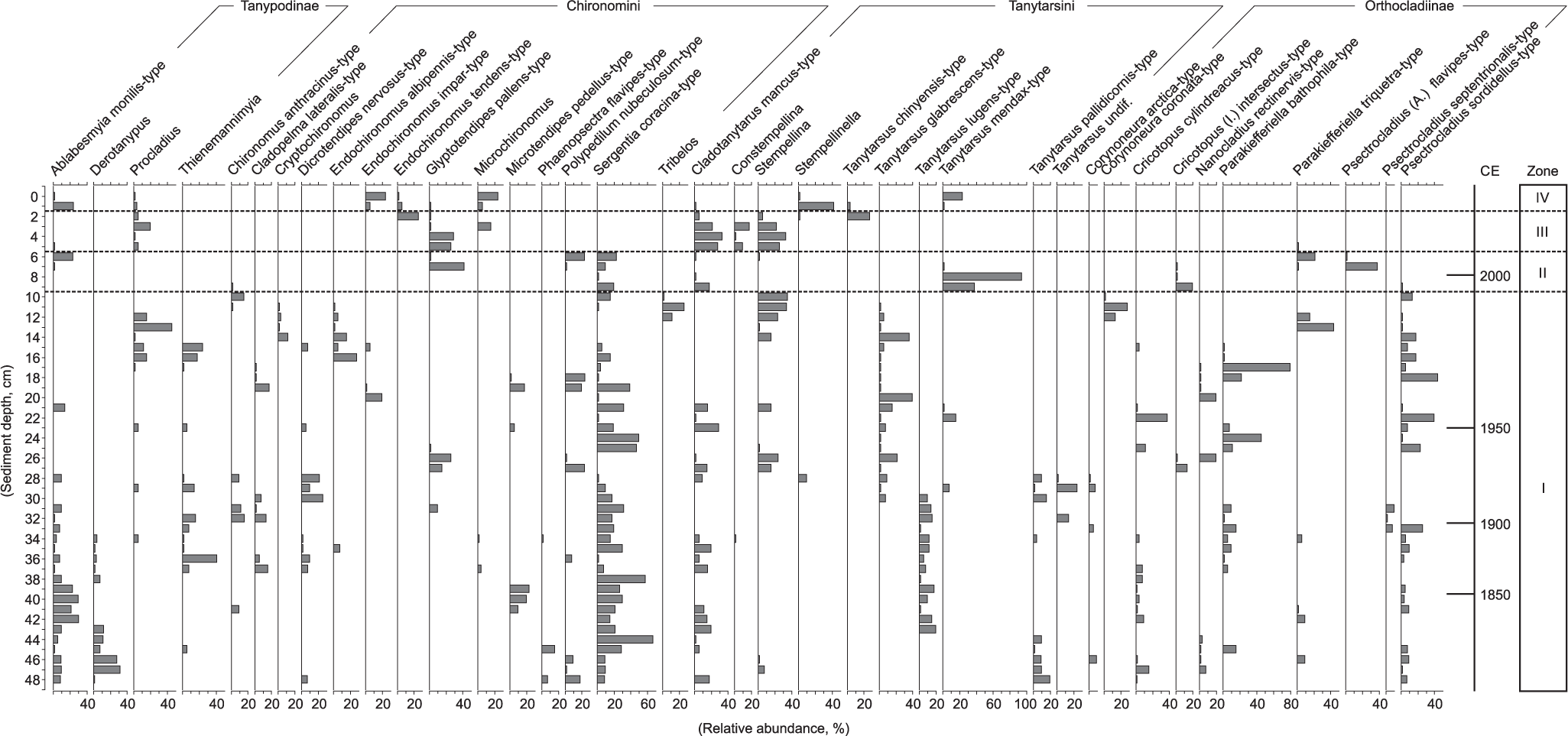
Relative abundance of the most common fossil chironomids in the varved lake sediments of Nurmijärvi.
The temperature optima of the most common chironomids had similar trends in both the CiT and CiS datasets (Figure 3). However, in case of every taxon, the CiT optima were consistently higher (0.7–3.4°C). The largest differences (>3°C) between the datasets occurred in Thienemannimyia, S. coracina-type, T. lugens-type, and Procladius.
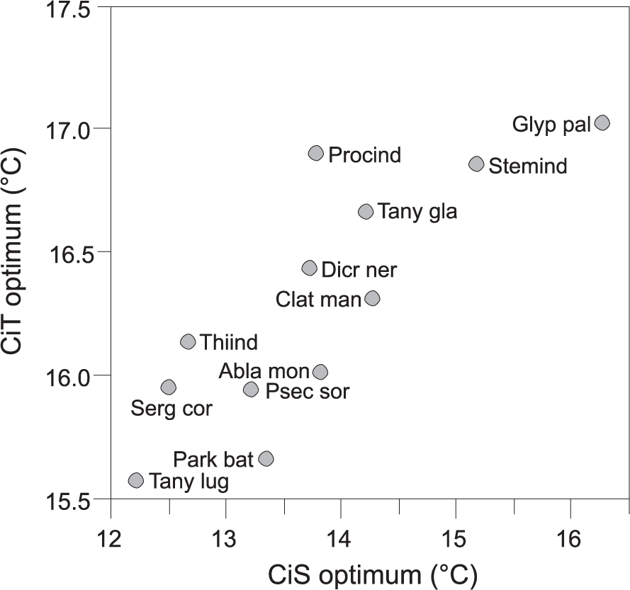
Weighted-averaging temperature optima of the most common chironomids (N2>5) in the Lake Nurmijärvi calibration-in-time (CiT) dataset compared against their optima in the calibration-in-space (CiS) dataset. The taxa codes correspond to the first four letters of the genus name and first three letters of the species name.
The first two PCA axes for chironomids were significant, the first axis (λ = 0.163) explaining 34.9% and the second axis (λ = 0.101) 21.6% of the total community variance. The PCA axis 1 scores varied between −0.54 and 0.78. All the samples dating prior to 1920 CE had negative axis 1 scores, whereas the subsequent samples had mostly positive scores (Figures 4 and 5). A significant correlation was found between the PCA axis 1 scores and the instrumental temperature record (R = 0.47, p = 0.002), suggesting that there is potential to develop a CiT model.

Instrumentally measured mean July air temperature (TJul) adjusted for the study site, principal component analysis (PCA) axis 1 scores for chironomids in the Nurmijärvi sediment core, and chironomid-inferred TJuls using the calibration-in-time (CiT) and calibration-in-space (CiS) approaches. The gray vertical lines represent the record-specific mean value, and the sample-specific errors in the reconstructions are assessed using bootstrapping cross-validation. Correlations (R) between the instrumental and inferred temperatures and the associated levels of statistical significance (corrected p) are also shown.

Principal component analysis (PCA) axis 1 and 2 scores for chironomids; magnetic susceptibility; organic matter percentage (measured as loss on ignition, LOI); ratio of fish scales, stream insect (mayflies and caddisflies), and Chaoborus mandibles (chaob:chir index) to chironomid head capsules; and the relative abundance of profundal chironomids in the Nurmijärvi sediment core. The horizontal lines represent significant faunal changes in the record identified by cluster analysis.
Of tested model types, WA with taxon tolerance weighting and inverse deshrinking regression showed best model statistics and was considered suitable for the nature of the data. This model had an r2jack of 0.64, an RMSEP of 0.55°C, and a maximum bias of 1.00°C. Compared with the CiS model, the CiT has lower predictive power and higher maximum bias but it outcompetes the CiS model in its prediction error (Table 1).
Descriptive statistics for the chironomid-based temperature inference models using calibration-in-time (CiT) and calibration-in-space (CiS).
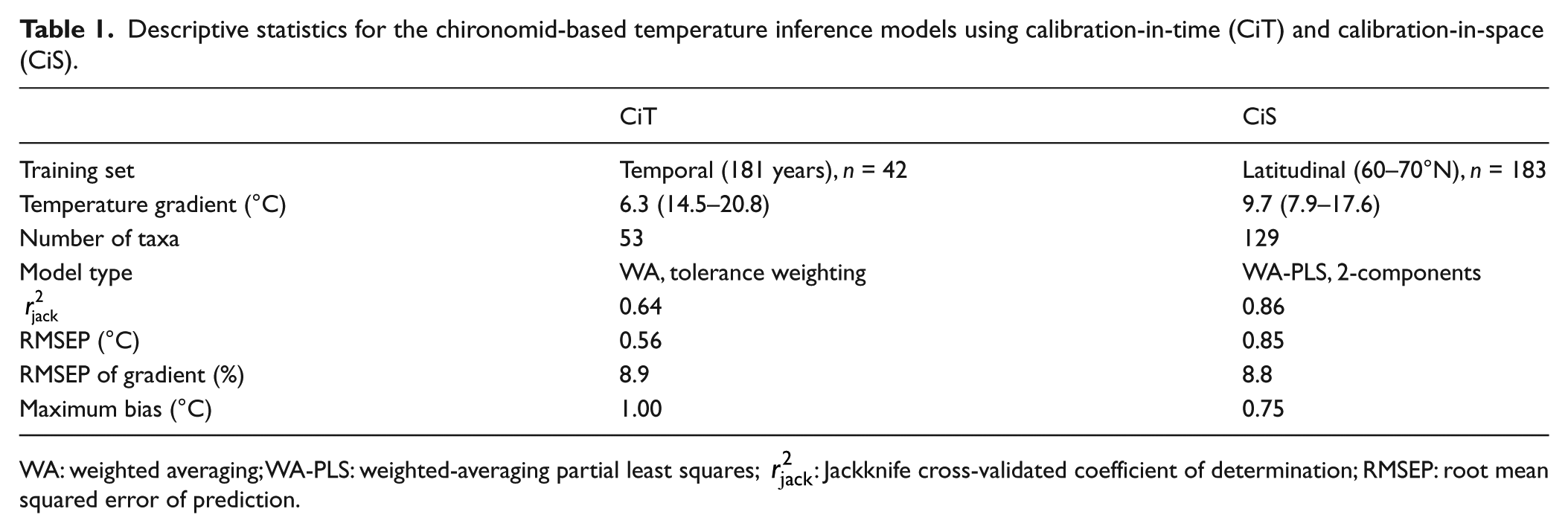
WA: weighted averaging; WA-PLS: weighted-averaging partial least squares; r2jack: Jackknife cross-validated coefficient of determination; RMSEP: root mean squared error of prediction.
The chironomid-based reconstruction using the CiS approach varied between 11.7°C and 20.7°C and the reconstruction using the CiT approach between 15.2°C and 18.8°C, both following the trends identified by the chironomid PCA axis 1 scores and the instrumental temperature record (Figure 4). However, the CiS reconstruction showed more intermittent temperature development compared with the smoother CiT reconstruction. A statistically significant relationship was found between the CiS reconstruction and the instrumental record (R = 0.38, correctedp = 0.014) (Table 2). According to the Durbin–Watson test, there was no positive autocorrelation between the series (Durbin–Watson statistic = 1.63, p = 0.114). In addition, the CiT reconstruction was significantly similar to the instrumental record (R = 0.51, corrected p = 0.001) and had no positive autocorrelation either (Durbin–Watson statistic = 1.99, p = 0.483). However, statistically significant lags between Chironomid PCA axis 1 scores and the instrumental temperatures were found for sample intervals 1 and 2, which correspond to minimum of 1 (topmost samples) and maximum of 19 years (lowermost samples of the observational period) in our record. According to the sediment accumulation rate, one sample lag represents ~4-year and two sample lag ~8-year time span on average.
Statistical relationships between the measured mean July air temperatures (TJul) and chironomid-inferred temperatures using the calibration-in-time (CiT) and calibration-in-space (CiS) approaches. The tests include Pearson correlation (R), autocorrelation corrected level of statistical significance (p), and the Durbin–Watson statistic.

Discussion
Community variance
Since the sediment stratigraphy in Nurmijärvi consisted of annually laminated layers verified by independent dating methods and enough chironomid head capsules were found for quantitative community analysis, we were able to perform temperature reconstructions that were subsequently compared with the meteorological record. However, because of variable rate of sedimentation (i.e. varve thickness) and 1-cm sampling resolution where each sample contained five varves on average (ranging between 1 and 11), the instrumental data had to be averaged accordingly.
The chironomid assemblages in the sediment core did not seem to include many true cold indicators. Only T. lugens-type and S. coracina-type, which were found most abundantly in the lower part of the core and were absent in the more recent samples (Figure 2), are found near the cold end of the gradient in the Finnish latitudinal chironomid-temperature training set (Luoto et al., 2014a). These results are logical, since the study site is located closer to the warmer, southern part of the training set. In contrast, the biostratigraphy consisted of several species with very warm temperature preference (Brooks et al., 2007), such as Endochironomus species, G. pallens-type, and T. mendax-type, which were more common in the recent parts of the profile (Figure 2). These community patterns fit well with the observed temperature trends that are evidenced by the correlation between the instrumental record and chironomid PCA axis 1 scores (Figure 4) representing the primary direction of variance.
Although the primary long-term community variance in Nurmijärvi is clearly linked with the temperature oscillations, the latter part of the chironomid stratigraphy is surprisingly patchy (Figures 2 and 4), considering that the sample intervals only represent a time span between a year and a decade. This is also well reflected by the cluster analysis, which shows that all the significant zone borders are located in the upper sediment section representing the past 20 years (Figure 2). Previous studies have shown that the chironomid survival and distribution can be regulated by the availability of hypolimnetic oxygen (Brodersen and Quinlan, 2006). In this study, the sediment samples were derived from the hypolimnetic part of the lake, which most likely suffers from summertime oxygen deficiency allowing the preservation of laminated sediments. Therefore, the alternating presence and absence of the taxa in the upper half of the profile probably has something to do with oxygen availability, but the potential oxygen changes are difficult to track based on the chironomid assemblage composition since all the occurring taxa can be found from low oxygen lakes. There also seems to be no oxybiontic taxa present in the upper half of the record. In contrast, in the initial part of the record, the abundant and consistent occurrence of T. lugens-type suggests milder hypoxia (Millet et al., 2010). The chaob:chir values, which reflect hypolimnetic oxygen depletion (Quinlan and Smol, 2010), suggest that mild anoxia may have occurred through the record in Lake Nurmijärvi (Figure 5). During the past 20 years, the inferred anoxia appears to change concurrently with percentage of profundal chironomids (Figure 5) that also indicate that the profundal areas may have been temporarily inhabitable. It is noteworthy though that since development of visible seasonal laminae, such as in the entire examined Nurmijärvi sediment profile, requires anoxic hypolimnetic conditions, the deepwater areas have remained more or less stable throughout the record. In any case, changes in oxygen conditions and subsequent reflectance on chironomid communities do not mean that the chironomid-temperature signal would necessarily be compromised. A previous study from southern Finland (Luoto and Salonen, 2010) showed that the oxygen conditions in two boreal lakes with different limnological conditions (eutrophic vs oligotrophic) oscillated according to changes in air temperatures. Consequently, higher hypolimnetic oxygen values were found during cold climate periods, such as the ‘Little Ice Age’, whereas lower oxygen availability was associated with warm episodes, including the Medieval Climate Anomaly and the present warming. These results are similar to the current chironomid assemblage succession, suggesting that hypoxia has increased in the lake alongside climate warming during the past century.
In comparison to chironomid-temperature optima between the CiT and CiS datasets, the largest offset was found in Thienemannimyia, Procladius, T. lugens-type, and S. coracina-type that had >3°C lower optima in the CiS dataset (Figure 3). Thienemannimyia and Procladius are free-living and can tolerate wide temperature ranges at the genus level that probably explains the offset, but the differences in estimated temperature optima of T. lugens-type and S. coracina-type may be related to lake depth. Both T. lugens-type and S. coracina-type live in the profundal and are typical cold-indicating taxa (Brooks et al., 2007). Since Lake Nurmijärvi is deeper than most of the lakes in the CiS training set, its profundal area provides a colder habitat for these taxa compared with the shallower lakes of the CiS dataset at the same air temperature regime.
When setting the results into a context of direct human-induced catchment changes, there seems to be no clear response in specific chironomid taxa (Figure 2) to the known human activities, such as the artificial lowering of the lake level related to saw-mill activity in the 1920s and 1930s (Markkanen, 1968). Nevertheless, there is a concurrent change during the 1930s in PCA axis 1 scores and magnetic susceptibility, which reflects catchment originated changes possibly related to operation of the saw-mill. In the later part of the core, there is a synchronous increase in sediment organic matter and changes in chironomid PCA axis 1 and 2 scores following the 1990s (Figure 5). There is a commonly observed eutrophication-like response of aquatic communities from temperate (Manca and DeMott, 2009; Visconti et al., 2008) to arctic (Luoto et al., 2014c, 2015, 2016a) lakes superimposed on climate change. Based on the chironomid biostratigraphy and simultaneous increases in the share of organic matter and measured air temperatures, this phenomenon appears to be operating also in Nurmijärvi. In addition, recent fish introductions, reflected by the increase in fish scales (Figure 5), may have caused changes in the chironomid communities as suggested by PCA axis 1 scores. Since the number of stream insects (mayflies and caddisflies) remained very low during the entire examined time period (Figure 5), it appears that hydrological changes (stream conditions) close to the sampling site have remained small. Considering all the changes that have occurred in potential secondary environmental factors, it is apparent that most significant confounding influences on chironomid-based temperature reconstructions have occurred in the most recent sediment samples. Therefore, the inferences of the past ~20 years should be considered with caution.
The results also indicated that there is a slight statistically significant lag in the chironomid response to air temperature change. This may be related to the length of the chironomid lifecycle, since though multivoltine, bivoltine, and univoltine lifehistories are most common, many northern species require up to 7 years to complete their development (Pinder, 1986). The observed lagtime of ~4–8 years is nonetheless much shorter than with pollen, for example, which may lag behind several decades because of soil forming processes. It should also be noted that the lag appears not to be visually consistent through the record (Figure 4) and there is a possibility that the lag is partly related to uncertainties in the chronology (chronological error estimate ±2%).
Temperature calibration and reconstructions
The close relationship between chironomid stratigraphy and temperature development allowed the construction of a CiT model. The CiT model is based on less sites compared with the latitudinal CiS model and it also has shorter temperature gradient and contains significantly less taxa. The temperature optima of the most common chironomid taxa in the Lake Nurmijärvi record showed similar characteristics between the CiT and CiS datasets, though there was a systematic trend where the CiT optima were generally ~2°C warmer (Figure 3). This is related to the temperature gradients of the datasets, since in the CiT, the lowest measured temperatures reach only 13.9°C compared with 7.9°C in the CiS dataset. When considering this offset in a downcore temperature reconstruction, it is probable that the dataset would infer similar temperate trends but the CiT would provide lower values than the CiS approach. Based on the descriptive statistics of the models (Table 1), the CiT model has lower RMSEP, whereas the CiS model outperforms in its r2jack and maximum bias. These results describe a rather typical pattern, since the prediction power of a good model performance is usually related to the gradient length and the number of included samples and taxa, while lower modeling errors can originate from the opposite characteristics (Olander et al., 1999). Also in a previous comparison between chironomid-based CiS and CiT models from Switzerland (Larocque-Tobler et al., 2011), the prediction power of the spatial calibration was higher but the temporal calibration had improved prediction error, indicating that these differences are inherent. In the current data, when the RMSEPs of the CiS and CiT models are compared relative to the training set temperature gradients, they come out very similar (Table 1), suggesting that the gradient is indeed in a major role determining the modeling errors.
In the reconstructions of air temperatures using the CiT and CiS, both approaches showed correlation with the instrumental record and also with the chironomid PCA axis 1 scores. In case of the CiT, these relationships are of course intrinsic. When comparing the models’ output, the CiT model appears to be more accurate approach to reconstruct paleotemperatures from the Nurmijärvi shortcore, since it follows more closely the instrumental temperature trend over the past ~180 years (Figure 4). In the lower part of the profile, before 1930 CE, the CiS approach underestimates the temperature values, and in the samples from 1940s onwards, the values show more variability than expected based on the measured data (Figure 4). These features are not present in the CiT reconstruction and may be related to issues dealing with the modeling technique. The tendency of WA-PLS models to yield more extreme reconstructions in comparison with simple WA is known from previous studies (Toivonen et al., 2001; Walker et al., 1997). This phenomenon appears to be more common in low-diversity samples (Luoto et al., 2010). Although the ability of WA-PLS models to extrapolate the results can be beneficial when working with samples close to or beyond the training set environmental gradient, such as often during the early-Holocene or other extreme climate periods, it may also cause unrealistic variability to a reconstruction, as demonstrated by the present results (Figure 4). Likewise, the applicability of the CiT model, based on simple WA, can be compromised if the fossil chironomid communities drastically change earlier during the Holocene compared with the communities prevailing during the calibration period. In such case, the CiS model having larger taxa coverage and potentially better modern analogues together with the ability to extrapolate beyond the calibration set temperature gradient probably outcompetes the CiT model in its reliability.
Consistent with previous findings (Larocque-Tobler et al., 2011), the present results suggest that the CiT approach is probably most suitable for shorter time intervals, whereas the regional CiS training sets can be more applicable for Holocene scale reconstructions. For periods dating beyond the Holocene, continental CiS training sets (Heiri et al., 2011; Lotter et al., 1999) and training sets that take the influence of continentality into account (Engels et al., 2014; Self et al., 2011) are probably the most useful. Based on the findings, it can justified to use both CiT and CiS approaches, though long-term and large-scale changes should be considered with caution in CiT, whereas the CiS most likely require regression-based smoothing, such as LOESS.
Conclusion
In this study, we were able to make linkages between chironomid communities and air temperature changes during the past ~180 years in an annually laminated sediment record from Finland. Although the chironomid stratigraphy was possibly also influenced by co-occurring changes in human activity, nutrient conditions, hypoxia, and fish status, the climate signal on chironomids was strong enough to test the CiT approach to reconstruct paleotemperatures. The results showed that although the CiT model has lower prediction error, it suffers from lower prediction power compared with the regional CiS model. The reconstructed temperatures using both calibration approaches correlated with the instrumental record, but the CiS model inferred changes at larger magnitude that could have been expected based on the meteorological data. Despite that the CiT model outperforms the CiS model in the current test against measured temperature data, it may be less applicable at longer timescales when environmental conditions and communities change beyond the temporal training set. A short spanning time lag was also observed in chironomid response to temperature change corresponding to the life history and development time of many northern chironomid species. However, this lag was not consistent in the record and can be considered reasonable compared with other paleoclimate proxies. In future studies, when both CiT and CiS models are available, it can be recommended to use both approaches in conjunction. However, the reliability of the CiT model at longer timescales should be carefully assessed, whereas CiS reconstructions, when based on WA-PLS, probably need statistical smoothing because of the model’s tendency to extrapolate results when the inferences are based on low-diversity samples or the environmental conditions reach closer to the end of the training set gradient. Based on our results, we conclude that Nurmijärvi is an ideal site for a future study to investigate high-resolution regional paleoclimatic changes during the Holocene using fossil chironomid assemblages. High-resolution assessments of chironomid response to local and global factors over periods of available instrumental data are an important prerequisite to strengthen the relevance of chironomid-based temperature reconstructions for a more effective use in local, regional, and global paleoclimate reconstructions.
Footnotes
Acknowledgements
We are grateful for the constructive comments by the two anonymous reviewers who helped to improve the manuscript.
Funding
This work was supported by the Academy of Finland (Luonnontieteiden ja Tekniikan Tutkimuksen Toimikunta, grant #259343 to Antti EK Ojala) and the Emil Aaltonen Foundation (personal grant #160156 to Tomi P Luoto).