Equilibrium line altitudes along the Andes during the Last millennium: Paleoclimatic implications

Cordillera Vilcanota

The Cordillera Vilcanota (13°45′S, 71°05′W) is a small mountain range that extends east-west for almost 50 km and forms part of the eastern Cordillera of the southern Peruvian Andes (Mark et al., 2002) (Figure 1). Its highest peak is Nevado Ausangate (6372 m a.s.l.). The climate in this area is characterized by a single marked wet season during the austral summer months (DJFM) and a prolonged ablation season (Rodbell et al., 2009). Approximately 15 km to the southwest, at Quelccaya Ice Cap (the largest ice mass in the tropics), systematic meteorological observations at 5680 m a.s.l. have shown that the mean annual temperature in this area is approximately −4.1°C (2004–2013) (D. Hardy, 2015, personal communication) and that mean annual accumulation is 0.86 ± 0.15 m water equivalent (2005–2015) (Hurley et al., 2015). The Cordillera Vilcanota is composed of granitic, sedimentary, and volcanic rocks (Audebaud, 1973). Our study focused on a small valley glacier in the Jasccara Valley (13°48′S, 70°59′W; herein Vilcanota site, Figure 2a), located in the southeastern Cordillera Vilcanota. With an estimated area of 0.74 km², this alpine glacier is 1.3 km long and has a steep profile with elevations ranging from ~5450 to 5070 m a.s.l. The ELA in the north side of the range is estimated at 5100 m a.s.l. (Mercer and Palacios, 1977), just 30 m above the toe of the modern glacier.

Tapado glacier, Cerro Tapado

Cerro Tapado (30°08′S, 69°55′W), with a maximum elevation of 5536 m a.s.l., is located south of the climatic region known as the Arid Diagonal (De Martonne, 1934) (Figure 1). Although high elevations at Cerro Tapado sporadically receive summer precipitation from the southeast, most precipitation in this area is linked to winter cut-offs of cold air-masses from the Pacific (Ginot et al., 2002; Marengo et al., 2004; Vuille and Ammann, 1997). Despite being located in an arid and generally ice-free environment, the southeast slope of Cerro Tapado hosts an ~1.5-km-long glacier (Schotterer et al., 2003) (Figure 2b), which reaches elevations as low as 4700 m a.s.l. With a surface area of ~1.2 km², this glacier is the largest ice mass in the area. It has an estimated ELA of 5300 m a.s.l. (Kull et al., 2002). The forefield of Tapado glacier is occupied by several rock glaciers of different ages.

Cipreses glacier, Sierra del Brujo

Sierra del Brujo (34°36′S, 70°17′W) is a small range located in central Chile, in the transition zone between the arid Andes and extremely wet Patagonia (Figure 1). The region exhibits mild, wet winters (~4 months long) and dry summers. Summers are semi-permanently affected by a high-pressure cell over the southeast Pacific Ocean, which prevents precipitation belts from reaching the area. During the winter, the westerlies can reach this region and generate frontal and orographic precipitation (Bown et al., 2008). The closest meteorological station located in Sewell (34°05′S, 70°24′W, 2155 m), 40 km north of Sierra del Brujo, reports a mean annual temperature of 10.4°C and total annual precipitation of 891 mm (Dirección Meteorológica de Chile, 2001). The Sierra del Brujo, composed of granodioritic rocks, is one of the most glacierized regions in the Central Andes of Argentina and Chile. This study focuses on Cipreses glacier (34°34′S, 70°21′W; Figure 2c), which extends north-south for ~9 km through the middle of Sierra del Brujo, with elevations ranging from ~4340 to 2580 m a.s.l. Including tributary glaciers, Cipreses glacier comprises an area of ~21 km². The lower portion of the glacier is debris-covered. No information regarding the ELA has been estimated for this or other glaciers in the area.

Tranquilo glacier, Monte San Lorenzo

Monte San Lorenzo (47°35′S, 72°19′W) is an isolated granitic massif located ~70 km to the east of the southern limit of the Northern Patagonian Icefield, more than 165 km from the coast (Figure 1). This mountain is the third highest summit in the southern Andes with an elevation of 3706 m a.s.l. The Monte San Lorenzo area has a transitional maritime to continental climate with a wide-annual thermal amplitude and a narrow range of mean monthly precipitation (Falaschi et al., 2013). The closest meteorological station located in Cochrane (47°14′S, 72°33′W, 182 m a.s.l.), 30 km to the northwest of Monte San Lorenzo, reports a mean annual temperature of 8.1°C and total annual precipitation of 731 mm (Aravena, 2007).

Monte San Lorenzo is one of the most extensively glacierized mountains in the region, with an ice-covered area of ca. 139 km² (Falaschi et al., 2013). Based on satellite images from 2005 to 2008, Falaschi et al. (2013) estimated the snowline to be ~1700–1750 m a.s.l. on the western sector of the massif and ~1800 m a.s.l. on the eastern side. This study focuses on Río Tranquilo valley, a north-south oriented valley on the northern flank of Monte San Lorenzo. A recent glacier inventory shows the existence of 16 small glaciers (<5 km²) in the headwalls of the valley, adding a total ice surface of 15 km² (Falaschi et al., 2013).

Glacier reconstruction and chronology

Former glacier extents and paleo-glacier surfaces were reconstructed using moraines and trimlines. We analyzed aerial photographs, satellite imagery (ASTER, Quickbird), and digital elevation models (ASTER GDEM Worldwide Elevation Data) to identify and map glacial landforms (for details, see Supplementary material, Appendix 1, available online). All remote interpretations were field checked.

To constrain the age of the former glacial fluctuations, we determined direct ages of moraines using surface exposure (¹⁰Be and ³⁶Cl) dating. At the Vilcanota site, and Cipreses and Río Tranquilo glaciers, we collected rock samples (~1 kg) for ¹⁰Be measurements from the surface of boulders atop moraine crests. Our sampling focused on large boulder (preferably >1 m), well embedded in the moraine, and that did not show evidence of post-depositional movement, surface erosion, or exhumation (see Supplementary material, Appendix 2, available online). Samples were removed from boulder surfaces (upper 5 cm) using a hammer and chisel or the drill and blast method of Kelly (2003). Beryllium was isolated from whole-rock samples in the cosmogenic laboratory at Dartmouth College. ¹⁰Be/Be isotope ratios were measured at the Center for Accelerator Mass Spectrometry at Lawrence Livermore National Laboratory (CAMS LLNL). ¹⁰Be ages were calculated based on the methods incorporated in the CRONUS-Earth online exposure age calculator version 2.2, with version 2.2.1 of the constants file (Balco et al., 2008). ¹⁰Be ages were calculated using the Southern Hemisphere mid-latitude ¹⁰Be production rate documented by Putnam et al. (2010) in New Zealand, which has been shown to be valid for sites in Patagonia (Kaplan et al., 2011), as well as for high-altitude tropical locations (Kelly et al., 2015). ¹⁰Be ages were calculated with time-dependent scaling after Lal (1991) and Stone (2000), although other scaling schemes (Desilets and Zreda, 2003; Dunai, 2001; Lifton et al., 2008; Pigati and Lifton, 2004) agree within 5% (not shown). All ¹⁰Be ages were calculated assuming no erosion. This assumption is likely valid giving the relatively young moraine ages and since selected boulders exhibiting minimal evidence of erosion. ¹⁰Be exposure ages are shown and discussed with analytical errors only.

In the case of Tapado glacier, where the predominant rock type is quartz poor, we determined moraine ages using ³⁶Cl dating. The moraines were barren of large boulders, and therefore, we opted to sample cobbles (~10 cm in diameter) from the surfaces of moraine ridges and other geomorphic features. This approach has been shown to yield cosmogenic ages indistinguishable from those collected from boulders on the same moraine, if collected where exhumation from depth or temporary burial of the cobbles is unlikely (Briner, 2009). To determine the whole-rock chemistry of the samples, we conducted elemental analysis at Activation Laboratories, Ltd. (ON, Canada; see Supplementary material, Appendix 3, available online). Cl samples were processed and ³⁶Cl ratios and total chloride were measured by isotope dilution and accelerator mass spectrometry (AMS) at Purdue Rare Isotope Measurement (PRIME) Laboratory at Purdue University. Ages were calculated using the CRONUSCalc ³⁶Cl online exposure age calculator, Version 2.0 (Marrero et al., 2016) using the Lifton-Sato-Dunai (LSD) nuclide-dependent scaling scheme (Lifton et al., 2014), which has been shown to produce ³⁶Cl ages that agree well with similarly scaled, locally calibrated Holocene ¹⁰Be and radiocarbon ages at high-altitude, low-latitude sites (Phillips et al., 2016). To check the consistency between ³⁶Cl and ¹⁰Be ages reported, we also calculated the ³⁶Cl ages using a time-varying Lal (1991)/Stone (2000) scaling scheme, which yielded identical ³⁶Cl ages to the LSD scheme (within 1.2% on average, and well within analytical uncertainty). Only sample ages calculated with the LSD scaling scheme are reported here. We note that calibration sites for ³⁶Cl production rates, particularly for whole-rock samples in this age range, are sparse (Phillips et al., 2016), so all input variables are provided in CRONUSCalc format in the data repository for ease of recalculation using other schema and calibration datasets as they become available. All ³⁶Cl ages were calculated assuming zero erosion. We interpret all surface exposure (¹⁰Be and ³⁶Cl) ages presented as the start of glacial retreat from the moraine from which the sample was collected.

Additionally, at the Vilcanota site, we collected radiocarbon samples from organic remains embedded in a moraine ridge. Radiocarbon measurements were carried out at the National Ocean Science Accelerator Mass Spectrometry Facility (NOSAMS). All radiocarbon ages were converted to calendar years BP (cal yr BP) using CALIB 7.02 and the SHCal13 calibration curve (Reimer et al., 2013). After calibration, radiocarbon ages discussed in this paper were corrected in order to make them comparable to our cosmogenic dates; this implies using the year 2010 as our reference for the present (CE 1950 + 60 yr = CE 2010).

For this analysis, to make consistent comparisons, we focused on the most extensive glacial advance (outermost moraines) that occurred during the last millennium, as identified by our chronology. Hereinafter, we refer to this event as the last millennium maximum (LMM), recognizing that the timing of this event may differ among the study areas.

Modern and paleo-ELAs

Paleo-glacier surfaces were reconstructed based on marginal features that indicate the past extents of the glacier and the elevations of its former margins. We paid particular attention to identify geomorphic evidence indicating the presence of tributary glaciers that may have merged with the main glacier during the LMM. Such evidence would have an important impact on the reconstruction of paleo-surfaces and, in turn, on the calculation of the basin’s hypsometry. Finally, we reconstructed the LMM glacier surface by fitting a planar surface over the former margins of the glacier. This approximation, although it does not capture the typical glacier surface topography (i.e. convex near the terminus, horizontal at mid-elevations, and concave near the headwall), can be considered a first-order approximation. The hypsometry of the glaciers was calculated based on the ASTER GDEM2 Worldwide Elevation Data (1.5 arc-second resolution). Present-day ice extents were mapped using Google Earth images taken in 2013 and 2015 (see Supplementary material, Appendix 1, available online).

To determine modern and former ELAs, we apply the accumulation area ratio (AAR) method, which assumes that the accumulation area of a glacier occupies a fixed portion of a glacier’s total area (Porter, 2001). The ELA is calculated by applying an estimated AAR value to a hypsometric curve of the glacier. Thus, this method is not only easy to apply but also takes into consideration the hypsometry of the glaciers in the ELA estimation.

The AAR values, however, vary from one region to another (Benn et al., 2005; Benn and Lehmkuhl, 2000). For example, steady-state AAR values for mid- and high-latitude glaciers range from 0.5 to 0.8 (Meier and Post, 1962), with typical values between 0.55 and 0.65 (Porter, 1975). AAR values tend to be higher for the inner tropics (AAR = ~0.8, Kaser and Osmaston, 2002). To accommodate this issue, we calculated the ELA values using a range of ratios derived from previous studies (Table 1). For our tropical site, Cordillera Vilcanota, we used AAR values ranging from 0.7 to 0.8, which are considered representative for tropical glaciers (Kaser and Osmaston, 2002). For Tapado glacier, in the subtropics, based on recent mass balance data (Kinnard, C., 2012, personal communication) and modeling results (Kull et al., 2002), we used AAR values ranging from 0.4 to 0.5. Finally, for the two mid-latitude glaciers, Tranquilo and Río Cipreses, we applied the range of AAR values most commonly used for mid-latitude glaciers of 0.55–0.65 (Bahr et al., 2009; Porter, 1975).

The AAR method was designed to calculate ELAs for glaciers under steady-state conditions. Thus, the calculations of ELAs of modern glaciers, which we consider to reflect ‘transient’ conditions, are likely lower than the actual ELA. Calculating the offset between the transient (minimum) ELA value and the actual ELA value is outside the scope of this study, but might be the subject of future work.

The change in ELA was calculated by subtracting the modern ELA from the paleo-ELA, using the mean, minimum, and maximum AAR values estimated for each zone. This method assumes that the AAR value for each glacier remains the same from the LMM to the present. We also assumed that the differences in glacial extent and ELA among sites are driven by mean climatic conditions and not simply by stochastic climate variability.

We recognize that debris-covered glaciers exhibit a complex interaction with climate (e.g. Reid and Brock, 2010). ELA calculations could be affected by this issue; debris cover reduces ablation and can affect glacial response on short time-scales. However, only one of our study sites (Cipreses glacier) currently exhibits debris cover. Since this debris cover occupies less than 10% of the total ice surface, we suggest that its impact on our conclusions is negligible.

Paleoclimatic reconstruction

The difference between the modern and LMM ELAs provides the basis to reconstruct scenarios of climatic conditions (temperature and precipitation) using a surface energy and mass balance model (SEMB model; Rupper and Roe, 2008). Details, uncertainties, and validation of the SEMB model can be found in Rupper and Roe (2008) and Sagredo et al. (2014). Below we briefly summarize the model.

For a given set of climatic conditions at a location, the SEMB model uses nested surface energy balance and surface mass balance algorithms to seek the altitude at which there is both a surface energy balance and a mass balance, defined here as the modeled ELA. The surface energy balance model solves for the energy available for ablation at a monthly resolution, using the following equation:

Q m = S + L + Q s + Q l

where Q_m is the energy available for melting snow/ice, S is the shortwave radiation flux absorbed at the surface, L is the net longwave radiation flux, Q_s is the sensible heat flux, and Q_l is the latent heat flux. Heat conduction is neglected because it is likely small compared with the terms we considered (Kayastha et al., 1999). The detailed equations describing S, L, Q_s, and Q_l can be found in Rupper and Roe (2008) and correspond to energy balance equations commonly employed in glaciology (e.g. Cuffey and Paterson, 2010; Kayastha et al., 1999; Mölg and Hardy, 2004; Plummer and Phillips, 2003; Senese et al., 2012).

The surface energy balance algorithm seeks a surface temperature that balances the given monthly air temperature, such that surface shortwave radiation is equal to outgoing longwave radiation and turbulent heat fluxes. If the resulting surface temperature is less than zero, then melt is zero and sublimation is proportional to the turbulent latent heat flux. If the surface temperature is zero, then both melt and sublimation are zero. Finally, if the surface temperature required to achieve energy balance is greater than zero, then the surface temperature is forced back to zero and the excess energy is used to calculate total melt.

The total annual ablation is calculated as the sum of the monthly sublimation and melt. In the surface mass balance algorithm, the model seeks the air temperature whereby total annual ablation equals annual accumulation. The ELA is found by using the local lapse rate to calculate the altitude at which this air temperature lies. The local temperature lapse rate was calculated based on the difference between the temperature at the geopotential height closest to the surface and the temperature at the geopotential height one level higher, using National Centers for Environmental Prediction–National Center for Atmospheric Research (NCEP-NCAR) reanalysis data as input (Kalnay et al., 1996).

Here, we solve for the suite of combined temperature and precipitation perturbations that accommodate the ELA change since the LMM. Model parameters and constants are the same as in Sagredo et al. (2014).

For all required SEMB model climate inputs, we used gridded monthly climatologies from the period 1961–1990. In particular, we used the gridded climatological output from CRU CL 2.0 (New et al., 2002) (Table 2). CRU CL 2.0 is a 10′ latitude/longitude resolution dataset of mean monthly surface climate over global land areas, interpolated from station means for 1961–1990. This dataset provides high-resolution information regarding those climatological variables (2-m air temperatures, annual precipitation, relative humidity, and wind speed) that are likely sensitive to local conditions. Unfortunately, this dataset does not provide all necessary inputs for the SEMB model. The remaining inputs were obtained from the NCEP-NCAR reanalysis output (Kalnay et al., 1996) (Table 2). NCEP-NCAR reanalysis uses an analysis/forecast system to perform data assimilation (2.5° resolution) using past data from 1948 to the present. The monthly mean reanalysis output for the period 1961–1990 was linearly interpolated to a 10′ resolution, thus providing the monthly climatologies consistent with the CRU input data used. Although uncertainty exists with these datasets, especially at high elevations, Sagredo et al. (2014) showed that the combined use of high-resolution CRU CL 2.0 climatological data and NCEP-NCAR reanalysis output, applied to our SEMB, captures the spatial pattern of modern ELAs across the Andes.

OPEN IN VIEWER

Table 2.

List of the model variables and units used.

Variables		Units
CRU CL 2.0
Ta_2m	Monthly mean annual 2 m air temperature	°C
Acc	Monthly mean precipitation	m
RH	Relative humidity	%
v	Wind speed	m s−1
NCEP-NCAR
Ta_std	Standard deviation of monthly 2 m air temperature	°C
Acc_std	Standard deviation of monthly mean precipitation	m
P	Air pressure at surface	Pa
Swdown	Net incoming shortwave radiation at the surface	W m−2
LWdown	Downwelling longwave radiation	W m−2
Ta_GP	Pressure level temperature	°C
H_GP	Pressure level Geopotential Height	m
Elev	Elevation of the grid cells	m

NCEP-NCAR: National Centers for Environmental Prediction–National Center for Atmospheric Research.

LMM reconstruction

Below, we describe the general glacial geomorphology and chronology used to define past glacial extents at the four study areas, with a focus on the features interpreted to date to the LMM.

Vilcanota site

Geomorphic evidence suggests that glaciers ice in the Jasccara basin expanded and deposited a series of moraines on the valley walls and bottom. We identified at least six moraine complexes in the area (Figure 3a). The Jasccara I and II moraines are associated with advances of the glaciers at the headwalls of the basin (9 and 7 km upvalley). The Tributary I, II, and III moraine complexes are the result of glacial fluctuations of the small tributary valleys on the northeast slope of the Jasccara valley. The Aljachaya moraine complex, on the other hand, was deposited by a glacier flowing out of the Aljachaya valley.

OPEN IN VIEWER

Figure 3.

Moraine complexes: (a) Cordillera Vilcanota, (b) Cerro Tapado, (c) Río Cipreses valley, and (d) Río Tranquilo valley. Each line represents an individual moraine ridge. Considering the complexity of the landscape in the forefield of Tapado glacier, other geomorphic units were also identified in panel (b). The dashed line in panel (d) represents a subtle ridge plastered against the inner slope of the RT6 moraine complex; we suggest that this subtle ridge corresponds to the LMM.

We obtained two radiocarbon dates of peat embedded in the outermost ridge of the Tributary I moraine. One age from the top and one from the bottom of this peat deposit yield ages of 560–590 and 1120–1330 cal yr BP, respectively (Table 3). These ages suggest that peat was growing upvalley from the Tributary I moraines during these times and that ice was smaller than the Tributary I extent from ~1330 to 560 cal yr BP. The peat was likely incorporated into the moraine after ~560 cal yr BP as the glacier advanced over the area where the peat was growing. Thus, these dates represent maximum-limiting ages for the Tributary I moraines. These dates agree with four samples from boulders on the crest of the Tributary I moraines that yield ¹⁰Be ages of 720 ± 20, 310 ± 10, 240 ± 20, and 160 ± 10 yr BP (Tables 4 and 5, and Figure 4a), with progressively younger ages more proximal to the glacier. These ages constrain the timing of glacier retreat from the Tributary I moraine. Based on these data, we suggest that the Tributary I moraines mark the LMM ice extent at the Vilcanota site and that this occurred at <560 yr BP. Similar dates constrain the LMM at Quelccaya Ice Cap, confirming our findings (see section ‘Discussion’; Stroup et al., 2014, 2015).

OPEN IN VIEWER

Table 3.

AMS radiocarbon and calibrated ages from Vilcanota. All radiocarbon dates were converted to calendar years BP using CALIB 7.02 and the SHCal13 calibration curve (Stuiver and Reimer, 1993).

Sample	Lat. (°S)	Long. (°W)	Lab code	Material	δ13C value (‰)	14C yr BP ± 1σ	Median prob. (cal yr BP)	2σ range (cal yr BP)
PEc10-01-01	−13.816	−70.968	OS-84284	Peat	−26.35	1260 ± 35	1130	1060–1270
PEc10-01-04	−13.816	−70.968	OS-84200	Peat	−23.04	500 ± 20	510	500–530

AMS: accelerator mass spectrometry.

OPEN IN VIEWER

Table 4.

Geographical and analytical data for 10Be samples. Ratios are normalized to the 07KNSTD standard. Shown are 1σ analytical AMS uncertainties. Density = 2.6 gm/cm³. Samples were prepared at Dartmouth College. Carrier concentration = 1.314 ppt.

	Sample ID	CAMS number	Latitude (°S)	Longitude (°W)	Elevation (m asl)	Boulder height (cm)	Thickness (cm)	Shielding	Quartz wt. (g)	9Be Carrier (g)	10Be/9Be ±1σ (10−14)	10Be Conc. ±1σ (103 at g−1)
Vilcanota	PE10-01-02	BE32436	−13.8129	−70.9679	5016	180	2.1	0.994367	13.1379	0.1587	0.6222 ± 0.0461	6.60 ± 0.49
	PE10-01-03	BE32437	−13.8136	−70.9679	5015	160	1.9	0.994983	12.9529	0.1625	0.8889 ± 0.0620	9.79 ± 0.68
	PE10-01-05	BE32438	−13.8160	−70.9683	4959	80	1.8	0.988513	16.6620	0.1635	1.4529 ± 0.0644	12.52 ± 0.55
	PE10-01-06	BE32439	−13.8157	−70.9690	4968	80	1.4	0.987221	12.9576	0.1627	2.6716 ± 0.0996	29.45 ± 1.10
Cipreses	CC10-01-02	BE32414	−34.5470	−70.4202	1730	182	4.8	0.962666	17.1747	0.1627	1.0149 ± 0.0660	8.45 ± 0.55
	CC10-01-03	BE32407	−34.5463	−70.4206	1705	70	2.5	0.964482	20.2736	0.1626	1.4782 ± 0.0805	10.42 ± 0.57
	CC10-01-05	BE32415	−34.5459	−70.4194	1707	95	1.5	0.970388	20.2923	0.1626	0.9927 ± 0.0709	6.99 ± 0.50
	CC10-01-06	BE32416	−34.5505	−70.3948	2018	140	2.6	0.939738	31.2031	0.1622	6.2949 ± 0.2123	28.75 ± 0.97
	CC10-01-09	BE32417	−34.5508	−70.3951	1983	100	3.5	0.945451	23.6607	0.1648	2.7142 ± 0.1065	16.61 ± 0.65
	CC10-01-10	BE32408	−34.5489	−70.4094	1798	100	2.0	0.965425	22.7830	0.1619	16.4457 ± 0.3120	102.69 ± 1.95
	CC10-01-11	BE32409	−34.5489	−70.4092	1793	110	2.5	0.965281	33.7317	0.1621	1.6962 ± 0.0852	7.16 ± 0.36
	CC10-01-12	BE32410	−34.5448	−70.4255	1712	150	3.0	0.948674	23.6899	0.1618	1.7102 ± 0.0861	10.26 ± 0.52
	CC10-01-13	BE32411	−34.5468	−70.4247	1760	70	4.1	0.960604	23.5803	0.1621	1.3988 ± 0.0979	8.45 ± 0.59
	CC10-01-14	BE32418	−34.5478	−70.4194	1722	230	2.5	0.962559	27.5314	0.1622	1.2056 ± 0.0786	6.24 ± 0.41
	CC10-01-19	BE32412	−34.5390	−70.4200	1772	110	2.5	0.974641	34.1962	0.1622	45.1592 ± 0.8426	188.22 ± 3.51
Tranquilo	PC10-01-17	BE32431	−47.5278	−72.3912	1291	160	2.0	0.984082	27.5379	0.1623	12.6183 ± 0.2429	65.30 ± 1.26
	PC10-01-18	BE32432	−47.5273	−72.3912	1281	100	1.3	0.977047	35.7078	0.1620	16.7384 ± 0.4178	66.68 ± 1.66
	PC10-01-19	BE32433	−47.5270	−72.3912	1277	110	2.7	0.980356	37.7215	0.1616	16.4104 ± 0.3069	61.73 ± 1.15

AMS: accelerator mass spectrometry.

OPEN IN VIEWER

Table 5.

¹⁰Be ages (yr BP) from Vilcanota, Cipreses, and Tranquilo sites. Ages calculated based on methods incorporated in the CRONUS-Earth online exposure age calculator, version 2.2, with version 2.21 of the constants file (see text, Balco et al., 2008), which includes renormalization of Table 3 results relative to 07KNSTD (Nishiizumi et al., 2007). Ages were calculated using the time-dependent version of Stone/Lal scaling scheme (Lal, 1991; Stone, 2000) with the production rate of Putnam et al. (2010). We report internal and external uncertainties that include scaling to the latitude and altitude of the sites.

	Sample	Age	int	ext
Vilcanota	PE10-01-02	160	10	10
	PE10-01-03	240	20	20
	PE10-01-05	310	10	20
	PE10-01-06	720	20	30
Cipreses	CC10-01-02	780	50	50
	CC10-01-03	950	50	60
	CC10-01-05	640	40	50
	CC10-01-06	2160	70	90
	CC10-01-09	1270	50	60
	CC10-01-10	8050	150	230
	CC10-01-11	630	30	30
	CC10-01-12	950	40	50
	CC10-01-13	760	50	60
	CC10-01-14	580	30	40
	CC10-01-19	15020	280	430
Tranquilo	PC10-01-17	5520	100	160
	PC10-01-18	5690	140	190
	PC10-01-19	5330	100	150

OPEN IN VIEWER

Figure 4.

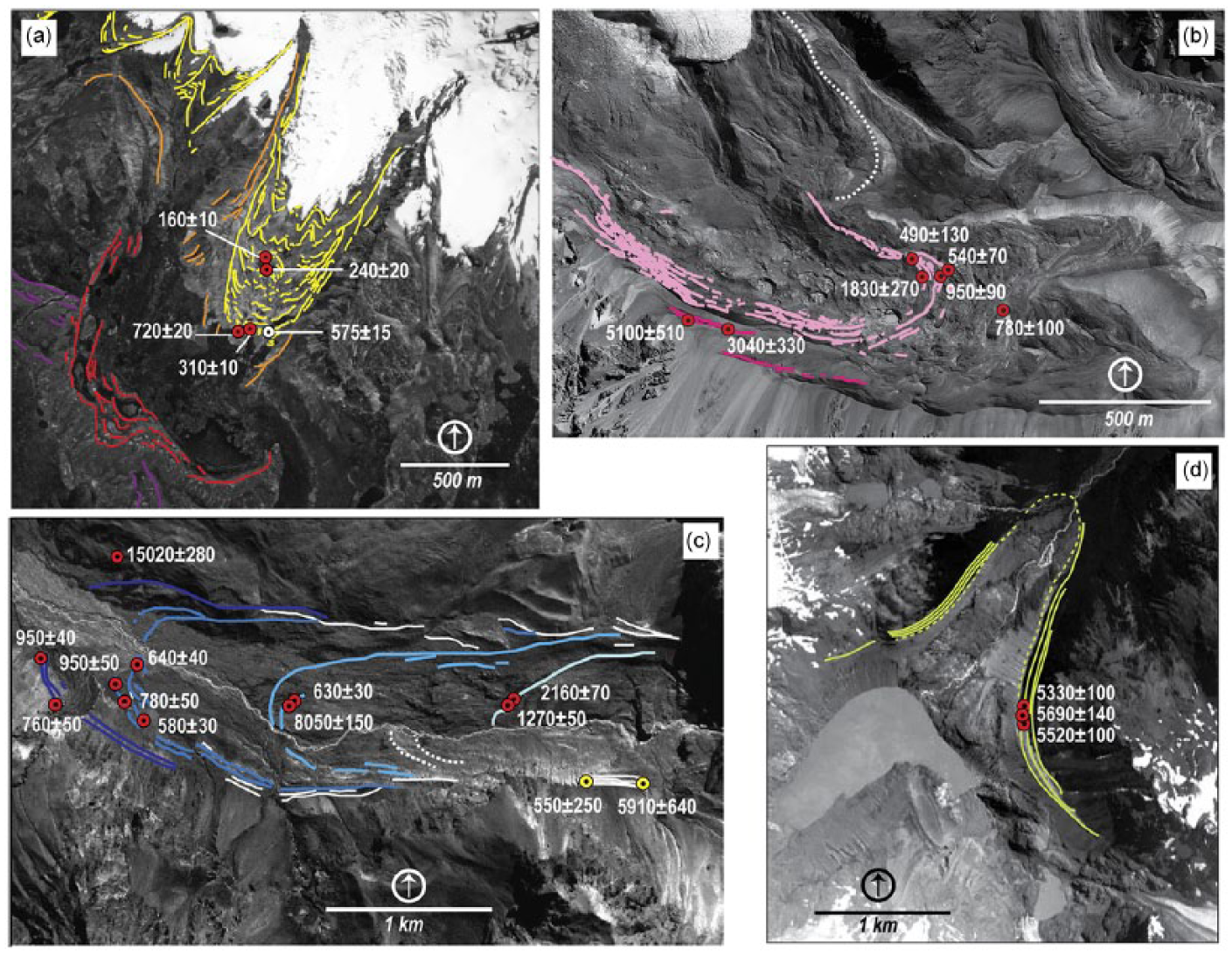
Dates constraining the age of the most prominent glacial advance that occurred during the Last Millennium Maximum (LMM) at each study site: (a) Cordillera Vilcanota, (b) Cerro Tapado, (c) Río Cipreses valley, and (d) Río Tranquilo valley. Red and white circles represent the location of the cosmogenic (ka) and radiocarbon ages (range of cal yr BP) obtained in this study, respectively. Yellow circles show the location of radiocarbon ages (cal yr BP) from Röthlisberger (1987).

Tapado glacier

As is common in lower precipitation regions, landforms below the glacier accumulation area also include mass wasting features. Debris-covered ice, ice-cored moraines, lobulated (and lineated) terrain, and several generations of massive rock glaciers occupy the forefield of Tapado glacier (Figure 3b). We distinguished a series of semi-continuous conspicuous moraine ridges (1–4 m high) that form an elongated arch in the forefield of Tapado glacier (Figure 3b, in pink) that appear to have undergone minimum disturbances since formation. We interpret this unit (herein: Tapado I) as a moraine complex formed by an advance of Tapado glacier over debris-covered ice. Distal to the Tapado I moraines are remnants of at least three or four older lateral moraines (Figure 3b, in fuchsia).

Four ³⁶Cl samples collected from the crest of Tapado I moraines yield ages of 490 ± 130, 540 ± 70, 950 ± 90, and 1830 ± 270 yr BP (Table 6, Figure 4b). One ³⁶Cl sample collected from the surface of an ice-cored moraine, just outside of the Tapado I moraine, resulted in an age of 780 ± 100 yr BP. Samples from the lateral Tapado II moraines yielded ages of 3040 ± 330 and 5100 ± 290 yr BP. Despite the scatter in these dates, we can distinguish at least two groups of ages: one group associated with the Tapado I moraine, with ages ranging between 500 and 1000 yr BP (one outlier), and another group associated with the Tapado II moraines, with two ages that are considerably older. Based on these results, we suggest that the Tapado I moraine was deposited sometime during the first half of the last millennium and that it represents the LMM limit. The Tapado II moraine, on the other hand, was probably deposited by a single or multiple glacial advances during the Holocene, prior to the deposition of Tapado I (the scatter of the ages precludes further interpretation)

OPEN IN VIEWER

Table 6.

Geographical and analytical data and ages for the 36Cl samples. Ages calculated using CRONUSCalc online calculator (Marrero et al., 2016) using Lifton-Sato-Dunai scaling (Lifton et al., 2014). We report external uncertainties.

Sample name	Sample Id	Latitude (°S)	Longitude (°W)	Elevation (m a.s.l.)	Thickness (cm)	Shielding	Cl in rock (ppm)	36Cl/Cl (10−15)	36Cl concentration (105 at/g rock)	Age (years)
NC11-01-11	201201394	−30.1568	−69.91927	4423	2	0.976965	30.03482	62 ± 8	0.32 ± 0.06	490 ± 130
NC11-01-12	201201395	−30.1571	−69.91894	4543	6	0.979958	18.91351	187 ± 11	0.60 ± 0.05	1830 ± 270
NC11-01-21	201201396	−30.1584	−69.92498	4618	3	0.922875	20.35587	462 ± 21	1.60 ± 0.11	5100 ± 510
NC11-01-22	201201397	−30.1587	−69.92432	4612	5	0.944775	21.92102	318 ± 14	1.22 ± 0.08	3040 ± 330
NC11-01-30	201201398	−30.1573	−69.91828	4538	7	0.978667	10.5315	91 ± 5	0.17 ± 0.01	950 ± 90
NC11-01-32	201201399	−30.1573	−69.91814	4537	4	0.980437	12.68254	63 ± 3	0.14 ± 0.01	540 ± 70
NC11-01-33	201201400	−30.158	−69.91665	4526	6	0.984819	11.67535	98 ± 6	0.21 ± 0.02	780 ± 100

Modern and paleo-ELAs

Based on the ice margins delineated in Figure 5, we estimated the present and LMM ELA for each glacier. Table 7 reports the ELAs corresponding to the preferred AAR value for each region. Figure 6 shows the range of ELA changes using the preferred AAR values.

OPEN IN VIEWER

Figure 5.

Oblique Google earth image showing the present-day (blue) and Last Millennium Maximum (red) ice margin: (a) Cordillera Vilcanota, (b) Cerro Tapado, (c) Río Cipreses valley, and (d) Río Tranquilo valley. Orientation of the images is shown by the circled arrows, which point to the North.

OPEN IN VIEWER

Table 7.

Modern and LLM equilibrium line altitudes. Values were calculated using different AAR values (see the ‘Methods’ section).

	Vilcanota		Tapado		Cipreses		Tranquilo
AAR	0.7	0.8	0.4	0.5	0.55	0.65	0.55	0.66
Modern ELA	5245	5195	5255	5195	3715	3645	1895	1835
LMM ELA	5105	5065	5115	4975	3615	3485	1765	1665
Delta ELA	140	130	140	220	100	160	130	170

OPEN IN VIEWER

Figure 6.

Hypsometry of the studied glacier. Solid lines represent modern hypsometry of the glaciers: (a) Cordillera Vilcanota, (b) Cerro Tapado, (c) Río Cipreses valley, and (d) Río Tranquilo valley. Dashed lines represent reconstructed hypsometry of the Last Millennium Maximum. Vertical dotted lines intersect the X axis in the AAR value selected for each site. Horizontal dotted lines intersect the Y axis in the corresponding ELA.

We estimated the following ELA changes from the modern to the LMM: Vilcanota site 130–140 m, Tapado glacier 140–220 m, Cipreses glacier 100–160 m, and Tranquilo glacier 130–170 m. When comparing the magnitude of these ELA changes, only the estimates for Vilcanota and Tapado glacier do not overlap.

Climatic implications

Next, we consider the range of possible combination of temperature and precipitation anomalies required to change the ELA from the modern to LMM values (Figure 7).

OPEN IN VIEWER

Figure 7.

Combination of temperature and precipitation anomalies (with respect to the present) that accommodate the ELA change from the Last Millennium Maximum to the present for the range of AARs used at each particular site. Color scheme is the same as in Figure 1. Inset: for reference, we included present-day temperature and precipitation variability (1σ) and values corresponding to 25%, 50%, 75%, and 100% of precipitation.

Assuming that ELA changes are because of only temperature, at the Vilcanota site, the ELA change can be explained by a cooling of at least 0.7°C. Considering a change in precipitation only, the LMM ELA can be explained by an increase of more than 0.52 m yr⁻¹ (representing a 64% of the present-day annual precipitation). At Cipreses and Tranquilo glaciers, the ELA changes can be explained by cooling of at least 0.6°C and 0.7°C or by precipitation increase of at least 0.22 (27%) and 0.30 m yr⁻¹ (27%), respectively. Finally, at Tapado glacier, where the maximum ELA depression was observed, the ELA change can be explained by a temperature decrease of at least 1.0°C (assuming no changes in precipitation) or by a precipitation increase of more than 0.31 m yr⁻¹ (89%, and no change in temperature). For the later site, negative anomalies of precipitation were not included because the SEMB model does not perform adequately when subjected to extremely low values of precipitation (Sagredo et al., 2014) (Figure 7).

Some of the changes in precipitation determined above could be considered unlikely. For example, at Tapado glacier, the change of precipitation required to decrease the ELA to its LMM elevation (without changing temperature) represents an increase in precipitation of 89%. For reference, Figure 7 (inset) shows the precipitation anomalies (m yr⁻¹) that represent a 25%, 50%, 75%, and 100% increase of annual values; in addition, we included the present-day temperature and precipitation interannual variability (±1 standard deviation of the mean conditions for the period 1961–1990).

Overall, the model results show that the range of possible temperature and precipitation anomalies that accommodate the observed ELA changes at all four sites studied show minimum overlap. Conversely, this overlap is very high when comparing only the glaciers at Vilcanota, Cipreses, and Tranquilo sites. This implies that the climatic anomalies responsible for the drop in ELA at Tapado glacier are the most distinct.

Chronology of the LMM

The chronology of the LMM relies on three different dating techniques, each of which has an analytical uncertainty (Tables 3, 5 and 6). The relatively small number of dates available from the various geological contexts makes use of formal statistical tests impractical at the moment (Balco, 2011). Nevertheless, we suggest that the post-depositional processes that may impact surface exposure ages (e.g. Applegate et al., 2012; Balco, 2011) are minimal because of the relatively short period of time that has passed since the LMM. Next, we contrast our dating results with prior studies where available.

On the northwest side of Cordillera Vilcanota, in the Upismayo valley, Mark et al. (2002) showed that the innermost moraine complex of the area was deposited after 340–560 cal yr BP (328 ± 46 ¹⁴C yr BP). In addition, at Quelccaya Ice Cap (15 km to the southwest of Vilcanota site), Stroup et al. (2014, 2015) showed that the LMM in the Qori Kalis and Chalpacocha valley occurred at >520 ± 60 yr BP. Similar results were obtained by Phillips et al. (2016), who constrained the LMM in the adjacent Huancané valley between 670 and 410 yr BP. These studies agree with our findings, supporting the idea that the LMM at the Vilcanota site occurred at <590 yr BP.

At Cipreses glacier, Röthlisberger (1987) radiocarbon dated two paleosols underlying lateral moraines in the upper portion of the valley (Figure 4c). The samples yielded ages of 5330–6610 cal yr BP (5180 ± 295 ¹⁴C yr BP) and 360–860 cal yr BP (625 ± 155 ¹⁴C yr BP), and represent maximum-limiting ages for the formation of the moraines. Unfortunately, these moraines are difficult to correlate with the aforementioned moraine complexes located downvalley, precluding comparison with the results of this study. Le Quesne et al. (2009) and Araneda et al. (2009) used historical records to infer that the Cipreses glacier margin was located near Medina II in CE 1842, implying that all the moraine complexes described above were deposited during the last ~170 years. Reexamining the evidence presented in these studies, we determined that the most conclusive record establishing the ice margin position comes from the description of Pissis’ expedition to the area. Pissis (1875) determined that by 1858, the ice margin was located at an elevation of 1758 m a.s.l. This suggests that Cipreses glacier was near the Arriero moraines, and that Medina I and Medina II moraines were ice-free by the time of this observation. This hypothesis can be extrapolated to 1842, considering that Araneda et al. (2009) determined that by that time the ice was only 100 m downstream from the position identified by Pissis. Based on this, as well as our new dates, we suggest that the Medina I and Medina II moraines were deposited during the first half of the last millennium (between ~950 and 550 yr BP).

At Tranquilo glacier, we obtained three consistent ¹⁰Be ages of ~5500 on the RT6 complex. These dates are statistically indistinguishable from the maximum age of 5280 ± 350 cal yr BP (4590 ± 115 ¹⁴C yr BP) obtained by Mercer (1968) for a glacial advance in the eastern flank of the same massif (47°36′S, 72°14′W).

Finally, the available dates suggest that while Tapado and Cipreses glaciers reached their LMM sometime during the first half of the last millennium, at Vilcanota this occurred at ~500 yr BP. We do not have chronological control over the LMM at Tranquilo glacier. Taken at face value, these preliminary data hint that the glaciers included in this study did not necessarily reach their LMM at the same time. However, we suggest that more chronological data are required to assess the synchrony (asynchrony) of these glacial events. For this reason, hereafter, we refer to the time when each glacier reached its maximum extent of the last 1000 years as the local LMM.

ELA estimates

ELA estimates for the study sites depend on reliable AAR values, which are known to vary from one climate regime to another. To overcome this problem, for each site we used a particular range of ELA values that are representative of each climate regime.

The results shown here suggest a significant overlap of the ELA changes across sites located in different climatic regimes along the Andes. Next, we compare our estimated ELA changes with previous studies. Note that the exact timing of the glacial events compared here may vary from site to site, but all reflect the ELA depression during the most extensive advance of the last millennium.

At the Vilcanota site, the estimated ELA change since the local LMM is in good agreement with those calculated for neighboring areas. To the south, in the Cordillera Real, Bolivia (16°S, Figure 1), Rabatel et al. (2008) calculated an ELA change of ~150 m since the local LMM (~AD 1650), with a total range of 70–190 m. This result is very similar to our findings for the Vilcanota site (ΔELA 130–140 m). To the north, in Cordillera Blanca, Peru (Figure 1), Jomelli et al. (2008) proposed that glaciers reached similar maximum extents in CE 1350 and 1650. The ELA change between these maximum extents and the modern day was estimated to be ~180 m (Jomelli et al., 2008), somewhat larger than the findings presented here.

At the Cipreses glacier, our results also agree with previous studies within the same climate regime. At the El Peñón and El Azufre glaciers, in Central Argentina (35°S, Figure 1) (Espizua, 2005), the change in ELA since the local LMM was estimated to be 105 and 110 ± 50 m, respectively. These estimations fall within the range of ELA changes calculated for Cipreses glacier (100 to 160 m). No other studies have reported LMM ELAs for the climatic region of Tapado or Tranquilo glacier, precluding further comparisons. At least for the climate zones occupied by the Vilcanota site and Cipreses glacier, it can be argued that our estimates for ELA are compatible with other published results, which would suggest that our sites are capturing a regional signal rather than local anomalies.

Climate reconstruction

The ELA changes described above were used to reconstruct scenarios of climatic conditions during the LMM. We used the SEMB model to calculate the combination of temperature and precipitation anomalies that accommodate the ELA changes since the local LMM. The SEMB model was designed for application in large regions (Rupper and Roe, 2008). Factors such as the spatial resolution of the model inputs, the selection and application of constants in different areas, and the omission of topographic (e.g. hypsometry and slope) and glacio-dynamic effects in the calculation of the ELA increase model uncertainties when applied to smaller areas or single glaciers (Rupper and Roe, 2008). However, if it is assumed that the ELA change at each glacier site is representative of its climatic region, which is supported by a comparison of our data with previous studies, the SEMB model provides a first approximation of the range of climatic conditions during the local LMMs in the study areas. The results indicate that the range of possible temperature and precipitation anomalies overlap significantly at three of the four sites. This implies that if we assume that the LMM was synchronous across these three study areas (Vilcanota, Cipreses, and Tranquilo sites), it is possible that the climate anomalies responsible for the LMM were similar in the southern outer tropics, northernmost mid-latitudes, and Central Patagonia. It is unclear to us whether the climate anomalies reconstructed for Tapado glacier are distinct because (1) of a true spatial variability in the climate conditions during the LMM, (2) we are actually comparing non-contemporaneous glacial events, or (3) because of problems in the delimitation of former ice margins, which would impact local ELA reconstruction.

It has been shown that glaciers in the Andes exist under various climatic conditions, which control their responses to climate change. By combining a geomorphological reconstruction of glacial advances, dating of these glacial advances, and applying the same SEMB model to glaciers located in different climatic regimes, we provide new insights toward the understanding of the climatic conditions that influenced glacier extents at their local LMMs along the Andes of South America. Our results fill information gaps and provide new data to understand Holocene climatic variability at a regional, hemispheric, and inter-hemispheric scale.