A 970-year-long summer temperature reconstruction from Rogen,west-central Sweden,based on blue intensity from tree rings

Abstract

To assess past climate variability in west-central Scandinavia, a new 972-year-long temperature reconstruction, based on adjusted delta blue intensity (ΔBI_adj), was created. Presently, it is the longest blue intensity chronology in Fennoscandia and the third longest in the northern hemisphere. Measurements were obtained from 119 tree line Scots pine (Pinus sylvestris L.) samples from Rogen, in the central Scandinavian Mountains, Sweden. Early and latewood blue intensity absorption data were used to create ΔBI_adj. The data were detrended using a signal-free regional curve standardization method (RSFi) to minimize biological noise and maximize low-frequency climate information. The Rogen ΔBI_adj chronology has a substantially stronger temperature signal at inter-annual timescales than the corresponding tree-ring width (RW) chronology, and it displays good spatial representation for the south-central parts of Scandinavia. The ΔBI_adj summer (June through August) temperature reconstruction, extending back to 1038 CE, exhibits three warm periods in 1040–1190 CE, 1370–1570 CE and the 20th century and one extended cold period between 1570 and 1920 CE. Regional summer temperature anomalies are associated with a Scandinavian–Greenland dipole sea-level pressure pattern, which has been stable for the past several centuries. Major volcanic eruptions produce distinct anomalies of ΔBI_adj indices indicating cooling of summer temperatures in the subsequent years. Our results show that ΔBI_adj from Pinus sylvestris in Scandinavia is a suitable proxy providing opportunities to explore past temperature variability at various frequencies, atmospheric dynamics and variability in external forcing. Nevertheless, long-term trend differences with RW imply that further research is needed to fully understand the application of this technique in dendroclimatology.

Keywords

1000 years blue intensity MXD Scandinavia temperature reconstruction tree rings

Introduction

To set the 20th-century warming in a long-term perspective, meteorological measurements are insufficient. Even though a few long observational temperature records spanning several centuries exist in Fennoscandia, for example, the Uppsala record reaching back to 1722 (Bergström and Moberg, 2002), such data are rare. Therefore, to access information about temperature variability beyond the late 19th century, climate proxies from various archives are needed. Tree-ring data are one of the most favoured natural archives for high-resolution multi-century to millennium-long temperature information. Indeed, most recent reconstructions of Northern Hemisphere temperatures have been based on tree-ring data, either exclusively (Anchukaitis et al., 2017; D’Arrigo et al., 2006; Esper et al., 2002; Frank et al., 2007a; Jacoby and D’Arrigo, 1989; Schneider et al., 2015; Wilson et al., 2007, 2016) or in combination with other proxies (e.g. Mann et al., 1999; Moberg et al., 2005). However, temperature-sensitive tree-ring data are not randomly distributed around the world, but in general confined to regions where trees are sensitive to temperature variability during the growing season, that is, close to or at the latitudinal or altitudinal tree lines (St George, 2014). Fennoscandia is in this sense an ideal environment to develop chronologies from various tree-ring proxies (Linderholm et al., 2010). It has one of the densest tree-ring networks in the world, where trees in the northern and west-central parts are highly sensitive to temperature (e.g., Hellmann et al., 2016; Linderholm et al., 2015), including several chronologies spanning 1000 years or longer (e.g. Wilson et al., 2016). Most temperature reconstructions have been developed in three key areas: (1) Torneträsk and (2) Finish Lapland in the north and (3) Jämtland in the west-central part of the region. The first reconstructions were based on tree-ring width (RW) data (e.g. Aniol and Eckstein, 1984). In recent decades, focus has shifted to maximum latewood density (MXD; Briffa et al., 1988, 1992; Grudd, 2008 (revised in Melvin et al., 2013); Björklund et al., 2015; Esper et al., 2012, 2014; Gunnarson et al., 2011; Matskovsky and Helama, 2014; Zhang et al., 2016) because of the superior and more spatially coherent temperature information obtainable from MXD compared with RW (Briffa et al., 2002). However, since producing MXD data is demanding, alternatives have been explored. McCarroll et al. (2002) discovered that blue light reflectance from scanned images of wood samples was a promising surrogate to X-ray measurements of wood density. This methodology, termed blue intensity (BI), has been further developed over the past few years (Björklund et al., 2014, 2015; Campbell et al., 2007; Rydval et al., 2014; Wilson et al., 2014). Working with Scots pine (Pinus sylvestris L.), Björklund et al. (2014) developed the ΔBI parameter, where the blue light absorption from the earlywood was removed from the maximum blue light absorption from the latewood to provide a stronger temperature signal focused on the summer season. Moreover, Björklund et al. (2015) found a systematic contrast difference between earlywood and latewood depending on the general discoloration of individual samples and suggested the use of a contrast-adjusted version of ΔBI termed ‘ΔBI_adj’. This method helps preserve low-frequency information that would otherwise be biased because of non-density-related changes in coloration in the samples. Presently, only a few reconstructions worldwide have included BI data: in Canada (Wilson et al., 2014), Scotland (Rydval et al., 2016) and Fennoscandia (Linderholm et al., 2015; McCarroll et al., 2013). However, only two reconstructions exclusively based on BI have been reported (Björklund et al., 2015; Dolgova, 2016). None of these cover the whole past millennia, except two BI chronologies, one from Khibiny in northwest Russia, extending over the past 1200 years, which was used in a Fennoscandian temperature reconstruction by McCarroll et al. (2013) and another dataset from central Europe with similar length which was used by Trachsel et al. (2012).

Most recent temperature reconstructions in Fennoscandia have been based on either MXD or a mix of MXD and BI data, predominantly sampled in the northern part of the region (>63°N). However, in order to gain a better understanding of past temperature variability for the entire region, Linderholm et al. (2015) showed that more data from the southern parts are needed. Despite the wealth of high-quality tree-ring temperature proxy records in Fennoscandia (e.g. Wilson et al., 2016), such data are still lacking for southern Scandinavia. Moreover, data from further south would provide means for extending and assessing the long temperature records from Stockholm and Uppsala, as well as providing a link to the European continent.

The aim of this study is to increase the knowledge of local temperature variability in west-central Fennoscandia as well as increasing the spatial data coverage further south. We introduce a ΔBI_adj chronology developed from Scots pine from the Rogen Natural Reserve in west-central Sweden, extending back to 980 CE. An earlier version of this data was used in the regional summer temperature reconstruction by Linderholm et al. (2015). The new chronology is compared with its corresponding RW chronology regarding temperature sensitivity, variability on different timescales and long-term trends. Based on the ΔBI_adj data, summer (June through August (JJA)) temperatures are reconstructed for the period 1038–2010 CE. The new reconstruction is set in the context of Fennoscandian temperature variability of the past millennium by comparing it to MXD-based summer temperature reconstructions from northernmost (Esper et al., 2012), east-central (Helama et al., 2014) and west-central (Zhang et al., 2016) Fennoscandia. Finally, we investigate the association between atmospheric circulation patterns, derived from observed and reconstructed sea-level pressure (SLP) data, and extreme summer temperatures in Fennoscandia on short and long timescales, as well as evidences of volcanic forcing in the ΔBI_adj data.

Material and methods

Sampling

The sampling of tree-ring material was conducted in Rogen Natural Reserve (62°22′N, 12°24′E) in the western part of central Sweden (Figure 1). The site is located just east of the main divide of the Scandinavian Mountains, in a region belonging to the Northern Boreal zone. A mosaic of mountain and lake systems characterizes the formerly glaciated area, with a topographic relief reaching between 1000 and 1270 m a.s.l. The climate of the region is classified as continental with a maritime influence and short summers. Monthly mean temperatures range from −10.6°C in January to 12.1°C in July, with an annual mean of 0.4°C (CRU TS 3.23 dataset, grid point 12°0′E; 62°N, 1901–2015 period mean). The total annual precipitation is 566 mm (CRU TS 3.24. 12°0′E; 62°N, 1901–2015 period).

Figure 1.

Map of the study area. The triangles indicate the locations of the Rogen study area and the nearby Jämtland chronology sampling area. Also shown (rectangles) are the areas where tree-ring data for N-Scan and H14 were sampled. The meteorological stations Trondheim and Uppsala are marked by squares.

A total of 230 Scots pine samples (radii) were collected at 700–900 m a.s.l. which is just below the local tree line (ca. 900 m a.s.l.) on the south-western slope of the mountain Handskinvålen. The site was characterized by an open forest with a patchy field layer vegetation, rocky outcrops, moraine ridges and hummocks and small lakes. The sampled living trees were growing on dry till soils, with an average age of 368 years. In order to minimize the influence of moisture fluctuations on tree growth, trees growing adjacent to lakes or in wet environments were not sampled (Düthorn et al., 2013; Linderholm et al., 2014). Both 10- and 12-mm increment borers were used to collect one to two cores per living tree at breast height (ca. 1.3 m), avoiding irregularities such as buttresses, branches, knots, possible damages and reaction wood. Additionally, discs were sawn from logs and stumps of dead trees.

At the Gothenburg Laboratory of Dendrochronology, the samples were mounted and sanded with progressively finer grades of sandpaper (40–1200 grit) until individual cells were visible under magnification (40×). Tree rings were visually cross-dated to their exact year of formation, and the widths of annual increments were measured with a 1/100 mm precision using a sliding measuring stage connected to the TSAP-Win software from Rinntech. The accuracy of the cross-dating was verified with the COFECHA software (Grissino-Mayer, 2001; Holmes, 1983), and the samples from the same trees were averaged into tree-ring series. A total number of 119 series were produced, whereof 48 series were derived from dry dead tree samples. Subsequently, the wood samples were prepared for BI analysis, where they were cut into 4-mm axial thickness laths and movable compounds extracted in a Soxhlet apparatus with 99% ethanol for 72 h (Björklund et al., 2015). After extraction, the samples were air-dried and sanded again (grit 1200).

Chronology construction

Images of the individual samples were produced with an Epson scanner (Perfection V600) using the scanner software SilverFast Ai Professional™ calibrated with an IT8.7/2 calibration target at a resolution of 1600 dpi. The commercial software WinDENDRO™ (Regent Instruments) was used to extract average blue absorption intensity data from the entire earlywood and maximum blue absorption intensity from the latewood. The BI earlywood and latewood parameters were subsequently adjusted for contrast following the protocol proposed by Björklund et al. (2015). In their study, measurements of BI were regressed on the corresponding x-ray density measurements from the same samples. The attained regression coefficients were found to be strongly associated with the sample average of earlywood BI, that is, the discoloration of the entire sample. By determining the average earlywood BI for each sample, we calculated the slope and intercept regression coefficients according to Björklund et al. (2015) which were then used to adjust the contrast between earlywood BI and maximum BI (that is the highest BI value in the ring equivalent to the maximum density in the densitometric measurements). Furthermore, ΔBI_adj was obtained by subtracting the adjusted earlywood BI values from the corresponding adjusted latewood MXBI values. The ΔBI_adj from different radii belonging to the same trees was also averaged, as for RW.

Standardization and statistical analysis

To preserve the low-frequency variance in the chronology used for the temperature reconstruction, a modified version of the multiple regional curve standardization (RCS; Briffa et al., 1992; Briffa and Melvin, 2011; Esper et al., 2002) termed RSFi (Björklund et al., 2013) was applied to the ΔBI_adj and RW datasets. It can briefly be described as follows. First, the tree-ring parameters were classified into groups of higher and lower than average growth, considering the whole series lengths (the proportion of high and low growth values was ~47% and ~53% for ΔBI_adj and ~43 and ~57% for RW). Then, signal-free (Melvin and Briffa, 2008), time-varying response-smoothing (Melvin et al., 2007) functions were obtained using the signal free software (Cook et al., 2014). The average values of these functions were adjusted to match the average value of the segment-length average of the assigned fast- or slow-growing regional curve groups. These functions were then used to calculate chronology indices through ratios for TRW (where the series are best characterized as heteroscedastic) and using residuals for ΔBI_adj (ΔBI_adj series are best characterized as homoscedastic; Fritts, 1976). In addition, we also produced chronologies using alternative detrending methods: traditional single RCS, with and without the signal-free approach, using the Sig-Free software (Cook et al., 2014).

The quality of the chronologies regarding common signal strength was assessed by means of the Rbar statistic, a measure of the common variance between the samples (Fritts, 1976) and the expressed population signal (EPS; Wigley et al., 1984). The RW and ΔBI_adj chronologies were compared regarding short- and long-term variability as well as trends. The common spectral characteristics were also assessed by a coherency test using the AnClim software (Stepánek, 2008), where the base length of the analysis was restricted to 10% of the chronology length. This analysis can be interpreted as the frequency-dependent squared correlation coefficient (Von Storch and Zwiers, 2004).

The climate signals in the tree-ring parameters were evaluated by computing Pearson’s correlation coefficients between RW/ΔBI_adj and monthly mean temperature and total rainfall. The analysis was based on monthly 0.5°×0.5° gridded CRU TS 3.23 data (Harris et al., 2014), using data from the closest grid point to the sampling site (62°N, 12°E). In addition, the low-frequency variations in the two chronologies were compared with observed temperatures from Uppsala 1722–2010 (59°51′N, 17°37′E, Bergström and Moberg, 2002) and Trondheim 1761–1981 (63°23′N, 10°30′E, retrieved from NOAA, https://www.ncdc.noaa.gov/ghcnm/). This was done by means of Pearson’s correlation on 10- and 20-year low-pass Gaussian filtered data. No adjustments of degrees of freedom were made.

Temperature reconstruction

For the ΔBI_adj-based temperature reconstruction, a transfer function was computed using simple linear regression, where the mean JJA temperature data were selected as the predictand and ΔBI_adj as a predictor (Fritts, 1976). A conventional split sample method (Snee, 1977) was used to calibrate and validate the reconstruction model, where the full observational data period (1901–2010) was split into two sub-periods (1901–1955 and 1956–2010) of equal length. To validate the quality of the model, the following statistics were used: reduction of error (RE) explained variance (R²) and coefficient of efficiency (CE; National Research Council, 2006). Additionally, the Durbin–Watson test was used to assess the autocorrelation of the regression residuals (Durbin and Watson, 1951), and the Cox and Stuart test (Cox and Stuart, 1955) was used for trend analysis. For the final reconstruction, calibration was performed over the full 1901–2010 period. To set the Rogen temperature reconstruction in a spatial context, the reconstruction was compared with a suite of previously published (Esper et al., 2012; Helama et al., 2014; Zhang et al., 2016), millennium-long, MXD summer temperature reconstructions from Fennoscandia.

Furthermore, JJA mean SLP patterns (data from the 20th Century Reanalysis dataset; Compo et al., 2006), associated with extreme summer temperatures (±1 standard deviation of high-pass-filtered data, same treatment for observed and reconstructed datasets) in the new reconstruction and observations (data from CRU TS 3.23, 1901–2010; Harris and Jones, 2014), during the 20th century were analysed by means of composite maps. The analysis was then extended back to 1659, using the SLP reconstruction by Luterbacher et al. (2002), to assess the long-term stability of the SLP-extreme temperature association. The mean responses of Rogen chronologies ΔBI_adj and RW to major volcanic events were assessed with superposed epoch analysis (SEA; Lough and Fritts, 1987). The analysis was based on three forcing series: Gao et al. (2008); Crowley and Unterman (2013) and Sigl et al. (2015), later referred to as G08, CU13 and S15, respectively. From each dataset, the 20 largest eruptions in the past millennium were considered (Supplementary Table 3, available online). Following Adams et al. (2003), the significance of the SEA was determined using a Monte Carlo block resampling (N = 10,000) of the actual event year windows.

Results

Chronology characteristics

Both RW and ΔBI_adj chronologies from Rogen, having identical sample depth through time, extend back to 980 CE (Figure 2). EPS levels of >0.85 are reached from 1073 to 2010 CE for the RW chronology and 1038–2010 CE for the ΔBI_adj chronology. The temporal evolution of the Rbar and EPS statistics is largely similar for the two parameters (Figure 2c). For example, drops in Rbar values are seen in the 1170s, 1400s and 1500s. The strength of the common signal is, however, higher for ΔBI_adj as indicated by the Rbar statistics (RW Rbar: mean = 0.47, min = 0.31, max = 0.67; ΔBI_adj Rbar mean = 0.51, min = 0.31, max = 0.82). The largest difference in Rbar between the two proxies occurs in the early part of the records, coinciding with the lowest sample depth. The RW data have a higher first-order autocorrelation (1-year lag) than ΔBI_adj parameter (r = 0.66 and r = 0.26, respectively).

Figure 2.

The Rogen chronologies (RW in black and ΔBI_adj in grey): (a) the temporal evolution of the two chronologies (z-scored) and their EPS values, (b) sample depth (number of trees) and Rbar statistics, (c) the low-frequency variability of the curves (z-scored chronologies smoothed with a 50-year low-pass Gaussian filter) and (d) coherence between RW and ΔBI_adj. The data were z-scored over the period 1900–2010.

At the beginning of the records (1000–1350), both chronologies display negative trends interrupted by sudden increases between 1350 and 1456. Following this period, ΔBI_adj presents a negative trend up to 1930, while RW displays a positive trend, showing a clear disagreement between the two records. At decadal scales, the two series co-vary, although RW displays higher decadal and multi-decadal variability compared with ΔBI_adj (s = 0.23 and s = 0.14, respectively, for RW and ΔBI_adj in RSFi versions; Figure 2c). In addition, both records show rather similar features during the past century, albeit RW is characterized by a steeper trend over this period. Additionally, the spectral properties suggest similar forcings of the two records. The coherence test (Figure 2d) reveals significant coherence (p < 0.01) at frequencies ranging between 58.6 and 15.8 years, and 10.8 and 8.2 years, but also at higher frequencies.

Comparing the temperature signal in RW and ΔBI_adj

The temperature signal in ΔBI_adj at inter-annual timescales is more pronounced than in RW. The former displays significant correlations with April–September temperatures, with a best-fit target season in JJA (Figure 3a). The RW parameter is significantly correlated with JJA temperatures, with a best fit for July temperature. Both ΔBI_adj and RW correlations with JJA temperature are significant (p < 0.05) over the 1901–2010 period. Furthermore, RW shows no significant precipitation signal (Figure 3b), while ΔBI_adj displays a significant, but weak, negative correlation with August precipitation. At lower frequencies, correlations between the chronologies and JJA temperatures from Uppsala (1722–2010) and Trondheim (1761–1981) showed no distinct differences between various chronology versions (RSFi; RCS with signal free and RCS without signal free, not shown), but it was indicated that (1) low-frequency temperature information is retained in ΔBI_adj and that ΔBI_adj contains a stronger temperature signal than RW also at longer timescales. For 10- (20)-year filtered data, the correlation between ΔBI_adj and Uppsala temperatures was r = 0.48 (0.4), compared with r = 0.35 (0.3) for RW. Using Trondheim, the correlation for ΔBI_adj was r = 0.35 (0.23) and for RW was r = 0.23 (0.17). Looking at the spatial representation of the temperature signal in the two chronologies (Figure 3c and d), there are notable differences between RW and ΔBI_adj in the strength of the field correlations with observed JJA temperature. Although both parameters show significant correlations across Fennoscandia, Denmark and the Baltic countries, the strength of the correlations is considerably higher for ΔBI_adj. The correlations for ΔBI_adj are strongest in southern Scandinavia, Denmark and south-western Finland, reaching up to 0.80 (p < 0.01) over the 1901–2010 period. The correlation weakens over northern Fennoscandia, but still reaches >0.5 except for the northernmost part. The correlation pattern for RW is similar to that for ΔBI_adj, but correlations are weaker, ranging between 0.4 and 0.55.

Figure 3.

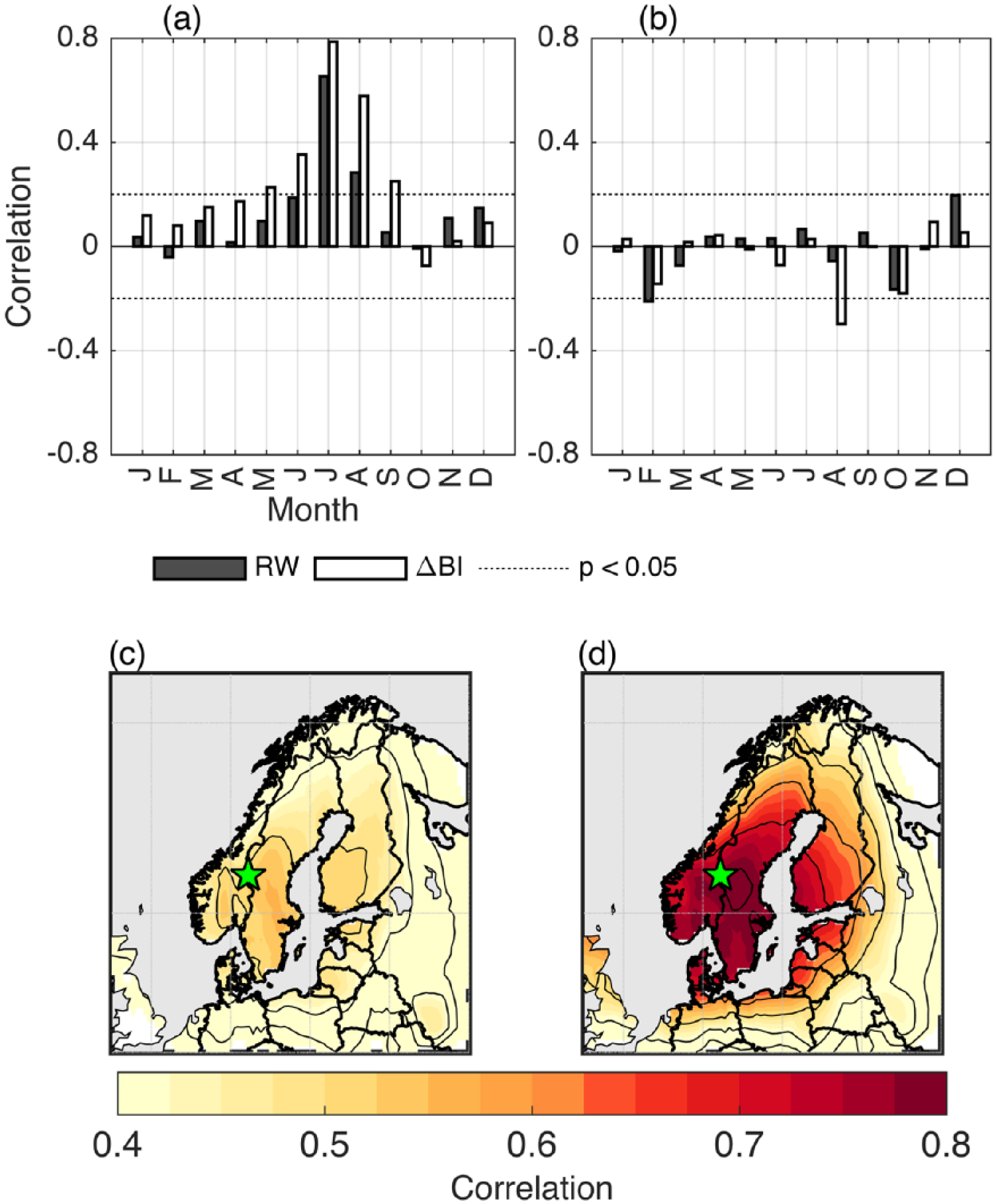
The climate signal in the Rogen RW and ΔBI_adj data, showing the correlations with instrumental observations (CRU TS 3.23; Harris and Jones, 2014) for (a) temperature and (b) precipitation. Spatial correlation between observations and (c) RW and (d) ΔBI_adj. All correlations were performed over the 1901–2010 period.

Temperature reconstruction

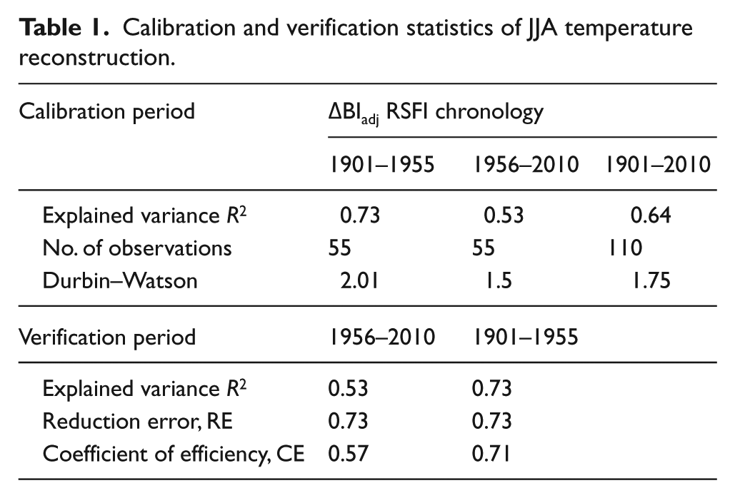
Because of the limited temperature signal and narrow target window of the RW chronology, we only used the ΔBI_adj chronology for a temperature reconstruction. The calibration and verification process showed that the relationship between the ΔBI_adj chronology and the CRU temperature data was stronger in the early (1901–1955: R² = 0.73, CE = 0.71, p < 0.01) compared with the late (1956–2010: R² = 0.53, CE = 0.57, p < 0.01) period. The R² value for the full 1901–2001 calibration period was 0.64, p < 0.01 (Table 1). Both CE and RE statistics were positive, indicating the model’s skills predicting observed temperature variability. The Durbin–Watson test indicated no autocorrelation of the regression residuals (see Table 1), and no significant trend was found in the regression residuals (Cox and Stuart test; p = 0.37).

Table 1.

Calibration and verification statistics of JJA temperature reconstruction.

Calibration period	ΔBI_adj RSFI chronology
	1901–1955	1956–2010	1901–2010
Explained variance R²	0.73	0.53	0.64
No. of observations	55	55	110
Durbin–Watson	2.01	1.5	1.75
Verification period	1956–2010	1901–1955
Explained variance R²	0.53	0.73
Reduction error, RE	0.73	0.73
Coefficient of efficiency, CE	0.57	0.71

The reconstructed JJA temperature record (Figure 4b) displays decadal and multi-decadal variability of temperatures during the past millennium. The reconstruction corresponds well with the previously reported chronologies from the area, with a warm period in the beginning of the record, corresponding to the Medieval Climate Anomaly (MCA), followed by colder conditions in the second half of the chronology, corresponding with the ‘Little Ice Age’ (LIA). The coldest decade, 30- and 50-year periods, was found during LIA, centred in 1709 (9.2°C), 1709 (9.6°C) and 1719 (9.8°C) (averages of JJA temperature). In turn, the warmest decade, 30- and 50-year periods, was centred in 1434 (12°C), 1436 (11.5°C) and 1421 (11.4°C) (average of JJA temperatures). From ca. 1850, a warming trend is observed extending into the 21st century, with maximum peak at 1937 (a list of warm and cold events is provided in Supplementary Table 2, available online).

Figure 4.

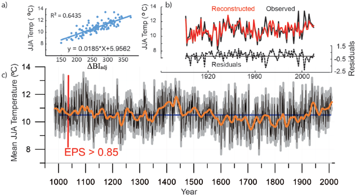
(a) Scatter plot of JJA mean temperature and ΔBI_adj data with a least square linear trend inset. (b) Comparison between observed (black) and reconstructed (red) mean JJA temperatures. (c) The full ΔBI_adj-based reconstruction of JJA temperature from Rogen. The bold line shows the 30-year Gaussian low-pass filter. The chronology mean (10.5°C) is represented by the blue horizontal line. Also shown are the ±1 root mean square error (RMSE) uncertainties (light grey lines). Red vertical line marks the EPS limit >0.85.

The magnitude and timing of the RW and ΔBI_adj responses to major volcanic events varied depending on the dataset used (Figure 5). Overall, the RW data showed a weaker and more muted response to volcanic events than ΔBI_adj. A significant response in RW chronology was only obtained when the CU13 dataset was used, showing significant growth depressions (ca −1.7 index anomalies) 4 years after the eruption. The ΔBI_adj chronology, in turn, revealed significant negative responses in the years after the event (ca. −2.5 index anomalies for CU13 and ~−2 index anomalies for G8 and S15). Using the CU13 data, significant negative responses of −2 index anomalies were also found in the actual year of the events, while the G08 data indicated negative response also in the second year after the events (also ~−2 index anomalies).

Figure 5.

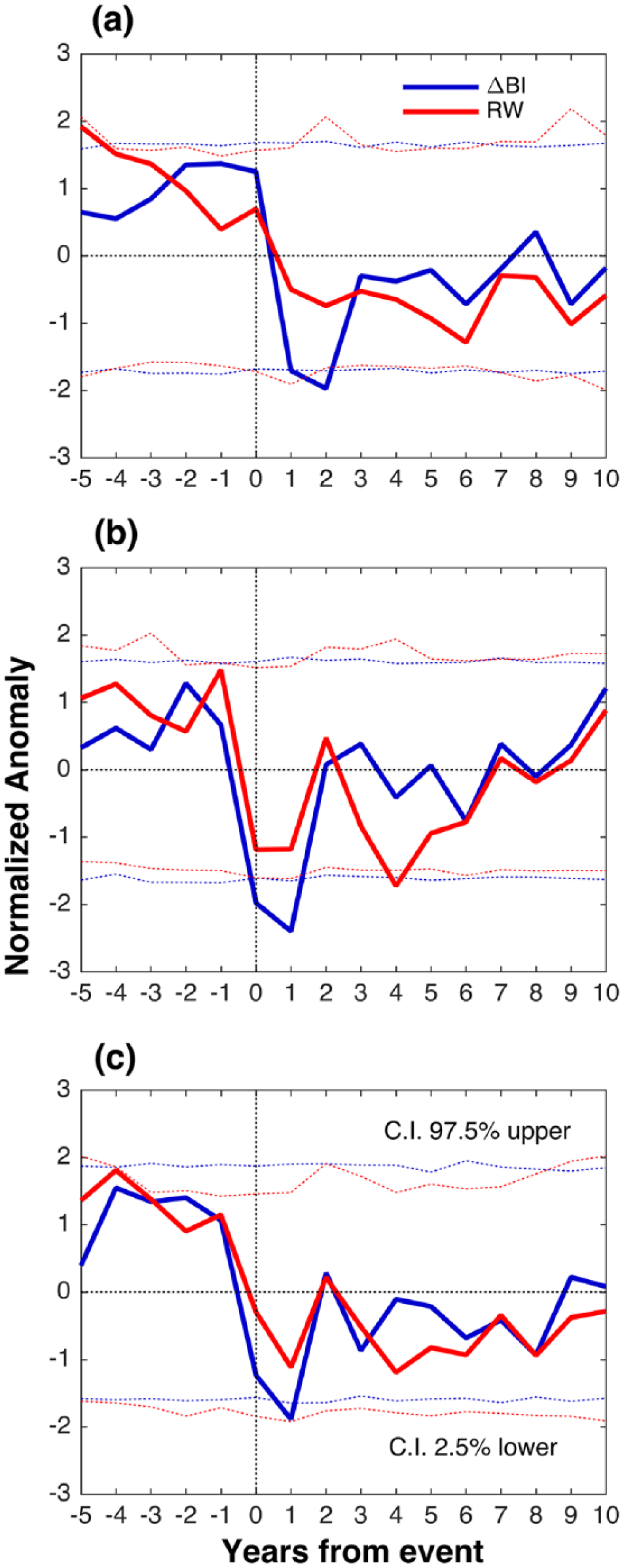
Superposed epoch analysis on RW and ΔBI_adj for three different datasets: (a) Gao et al. (2008), (b) Crowley and Unterman (2013) and (c) Sigl et al. (2015). Full lines indicate response to volcanic forcing for RW in red and ΔBI_adj in blue. 95% confidence envelopes are shown in dotted lines.

Synoptic patterns associated with extreme years

Based on our definition (see above), we found 16 (17) years of extreme positive years in the observational (ΔBI_adj) data and 17 years of negative JJA temperature extremes in both datasets between 1901 and 2010. It is worth noting that only seven of the positive extreme years were common for both observations and reconstructions, while 11 were common for the negative extremes. The SLP patterns associated with the extreme years in both datasets are given in Figure 6. The patterns are highly similar for both observed and reconstructed data, despite the mismatch between extreme years between the two datasets, and are mainly characterized by a dipole pattern over Fennoscandia and Greenland (Figure 6a–d). Positive JJA temperature extremes coincide with positive SLP anomalies over Fennoscandia (more pronounced for the observations) and negative SLP anomalies over Greenland (mainly for the reconstruction) and the Greenland Sea. Significant negative SLP anomalies are also found across southern Europe, especially for the reconstruction. Negative temperature extremes are associated with a negative SLP anomaly over Fennoscandia (again more pronounced for observations) and a prominent positive SLP anomaly over Greenland and the Greenland Sea. In addition, significant negative SLP anomalies are found over the NW Atlantic, outside eastern Canada for both observations and reconstruction, and a weak positive SLP anomaly in south-eastern Europe (only observations). These patterns are consistent when comparing the reconstructed Rogen temperatures to reconstructed gridded SLP over the European sector (Luterbacher et al., 2002) back to 1659 CE (Figure 6e and f), indicating that the observed patterns associated with JJA temperature extremes have been stable during the past several centuries.

Figure 6.

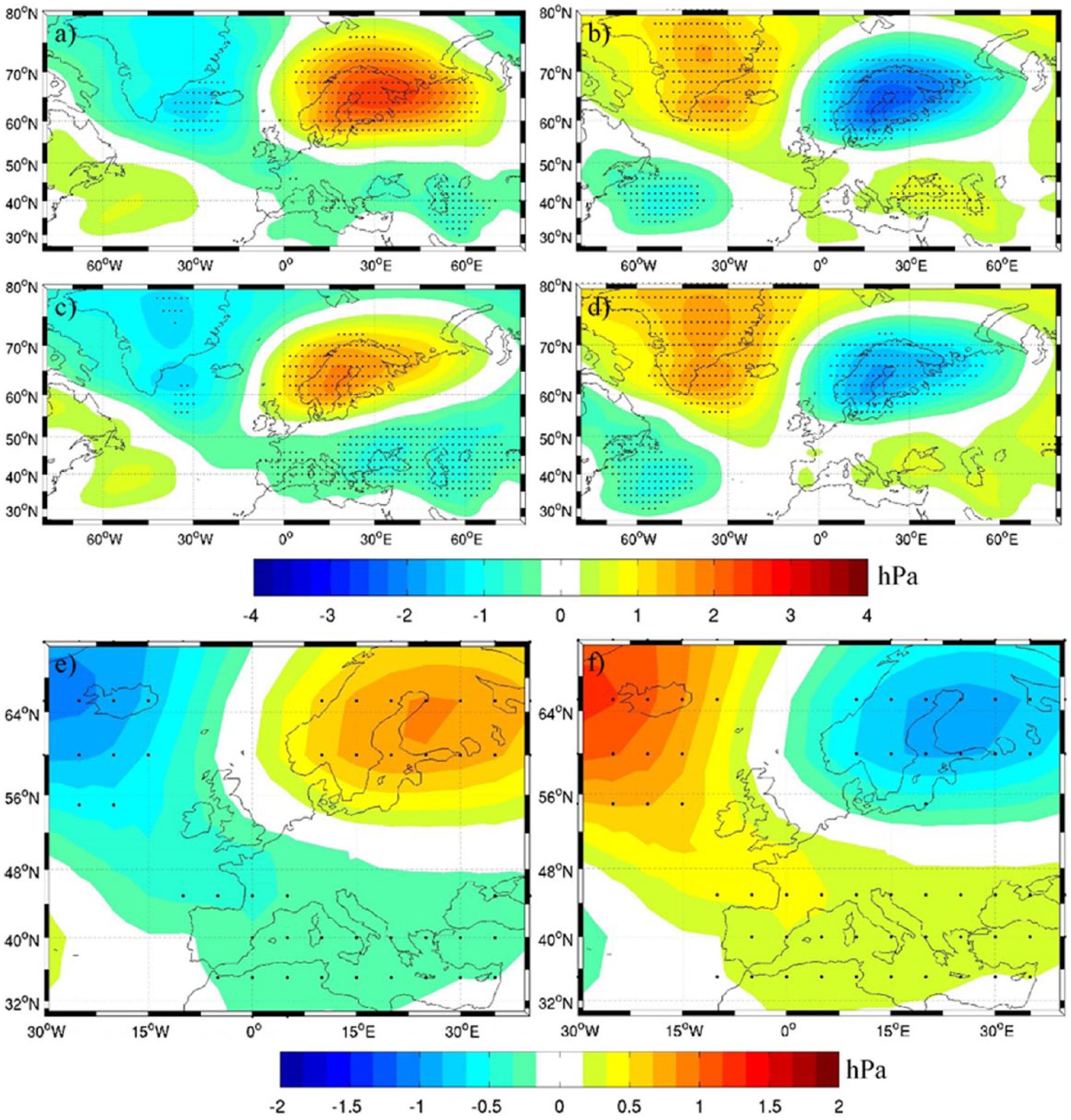
Composite fields of SLP 20th Century Reanalysis data (Compo et al., 2006, 2011) selected on extremes between 1900 and 2010 of (a) positive mean temperature extremes from CRU TS 3.23 data (Harris and Jones, 2014) (1901, 1912, 1914, 1917, 1930, 1933, 1936, 1937, 1945, 1947, 1953, 1969, 1997, 2002, 2003, 2006); (b) negative extremes (1902, 1907, 1921, 1923, 1928, 1929, 1931, 1952, 1956, 1962, 1964, 1965, 1981, 1987, 1993, 1998, 2000); (c) positive extremes of the high-pass-filtered Rogen JJA temperature reconstruction 1901–2010 (1901, 1906, 1910, 1914, 1925, 1927, 1930, 1937, 1947, 1955, 1959, 1973, 1975, 1980, 1988, 1994, 1997); (d) negative extremes of the high-pass-filtered Rogen JJA temperature reconstruction 1901–2010 (1902, 1907, 1909, 1923, 1928, 1929, 1931, 1942, 1952, 1958, 1962, 1971, 1977, 1979, 1987, 1993, 1998); (e) composite fields of reconstructed SLP (Luterbacher et al., 2002) based on dates of positive anomalous high-pass-filtered Rogen JJA mean temperature reconstruction 1659–1999; and (f) same as (e) but based on negative anomalies. Dots indicate local significance at the 0.05 level.

Discussion

Presently, Rogen is the longest temperature reconstruction based exclusively on BI data. Longer datasets include the ‘Khibiny’ record (821–2005 CE) from the Kola Peninsula in Russia, which was used in reconstructions by McCarroll et al. (2013) and Wilson et al. (2016), and an Austrian dataset (813–1996 CE) reported by Trachsel et al. (2012). Other BI reconstructions presented in Björklund et al. (2015), Rydval et al. (2014), Linderholm et al. (2015), Wilson et al. (2014) and recently Dolgova (2016) extend over shorter time spans but represent the increasing interest and potential of using this proxy for climate studies.

RW versus ΔBI_adj

One of the most attractive feature of the BI methodology is the high quality of the temperature signal in the higher frequencies (Björklund et al., 2014, 2015; Campbell et al., 2007; Dolgova, 2016; McCarroll et al., 2002; Rydval et al., 2014; Wilson et al., 2014). The inter-annual temperature signal is stronger in ΔBI_adj (Figure 3) than in RW and according to previous studies of similar strength as that in MXD (Björklund et al., 2014, 2015). Our results also show that ΔBI_adj data are more sensitive to volcanic eruptions than RW. It has been argued that tree-ring data underestimate the temperature impact of major volcanic eruptions compared with climate models (Mann et al., 2012, 2013). However, the volcanic forcing signal is pronounced in our ΔBI_adj chronology, being stronger than for RW (Figure 5). Depending on the volcanic eruption dataset used, the ΔBI_adj chronology suggests index anomalies of about −2 following an eruption, with the strongest effects in the year after the event (except for the G08 data, where the strongest effects are reached after 2 years). This is broadly in line with what has been found in other tree-ring-based reconstructions (e.g. Linderholm et al., 2015; Rydval et al., 2016; Stoffel et al., 2015), although the inferred cooling is generally lower when tree-ring networks are used. The weaker and marginally longer response of RW to volcanic forcing may be related to the higher persistence in RW data (as evidenced by higher first-order autocorrelation), also leading to slower recovery time (Esper et al., 2015; Franke et al., 2013).

One of the previously reported limitations of BI data is its reduced retention of low-frequency information, when compared with RW or MXD. Rydval et al. (2014) highlighted problems in the low-frequency signal of latewood minimum BI (MBI) measured from Scots pine because of the colour differences between heartwood and sapwood. Wilson et al. (2014) emphasized the possibility of long-term signal distortion related to detrending options and length of the used climate data, finding reduced fidelity of MBI to temperature at frequencies lower than 20 years. Nevertheless, we argue that the approaches presented in Björklund et al. (2013, 2014, 2015) allow us to retain useful low-frequency information using the ΔBI_adj parameter and careful standardization procedures. Our analysis indicates significant coherences between RW and ΔBI_adj on decadal to multi-decadal frequencies (Figure 2d), indicating that ΔBI_adj can overcome this inferred limitation of BI, as was also shown in Fuentes et al. (2016). This is further supported by higher correlation between ΔBI_adj and temperature data from Uppsala (1722–2010) and Trondheim (1761–1981), also at lower frequencies, and coherence analysis between Rogen chronologies and the climate data series shown in Supplementary Figure 3 (available online).

Another issue which became evident when comparing the RW and ΔBI_adj chronologies is the differences in long-term trends, which are more or less opposite over the past millennium (Figure 2c). The trend difference is unlikely an effect of detrending method, since it was similarly independent of the method used (Supplementary Figure 1a and b, available online). It is clear that RW and ΔBI_adj display greater trend differences for chronologies built only from living trees while almost no differences are observed for chronologies composed of subfossil material (Supplementary Figure 1c–g, available online). This means that the subfossil wood and living tree material have different average growths; the older RW material has narrower rings, and the latewood has a higher density or darker colour than the living material. This feature cannot be removed with standardization that preserves average differences across generations, and because it is unlikely with different trends in temperature data of JJA and July, the trend discrepancy of the two proxies likely diverges because of modern sampling bias (Briffa and Melvin, 2011; Melvin, 2004; Melvin et al., 2013) and it is greater when comparing indices derived from wood material from the living trees. Similar features can also be seen when comparing RW and MXD from C-Scan (Zhang et al., 2016) and N-Scan (Esper et al., 2012), which also display differing trends in RW and MXD chronologies (not shown). Arguing that ΔBI_adj contains a similarly strong temperature signal as MXD and that the adjustment method preserves low-frequency temperature information in the BI data consistent with that of MXD, the trend during the past millennium is more plausible in the ΔBI_adj chronology than in the RW one. This assumption is further supported by the trend of the ΔBI_adj chronology coinciding with those observed in many MXD datasets that have been claimed to be superior to RW (e.g. Esper et al., 2012; Melvin et al., 2013). In fact, the trend in the corresponding RW for Torneträsk (Melvin et al., 2013) is similar to those found in MXD data. Moreover, according to other proxy data, it is likely that the long-term temperature trend of the past millennium should have been slightly negative until the start of modern warm period (e.g. Esper et al., 2012; Jansen et al., 2007; Ljungqvist et al., 2012). Consequently, we argue that the ΔBI_adj data better capture the long-term trend of the regional temperature history compared with RW. Still, the reason for the systematic mismatch in trends of many MXD or ΔBI_adj records compared with RW records (Figure 2a–c, Supplementary Figure 1, available online) remains an open question and needs to be investigated.

The Rogen reconstruction in a Fennoscandian context over the past millennium

To set the new Rogen temperature reconstruction in a Fennoscandian context, it was compared with three previously published MXD-based temperature reconstructions from the region: Northernmost Fennoscandia (N-Scan, JJA; Esper et al., 2012), Southern Finland (referred to as H14, May–September; Helama et al., 2014) and the central Scandinavian Mountains (C-Scan, April–September; Zhang et al., 2016). On inter-annual timescales, there are good agreements between Rogen and other reconstructions, especially with N-Scan (r = 0.52, n = 972, p < 0.01) and C-Scan (r = 0.80, n = 938, p < 0.01), while the correlation with H14 is lower (r = 0.32, n = 928, p < 0.01). Considering the distance between the different chronologies, it was expected that Rogen would be more strongly correlated with C-Scan, than the more northerly and easterly records. This fact is further supported by the field correlations between the chronologies and observed temperature (Figure 3).

The temperature variability of the past millennium was characterized by three main warm episodes: a warm period during the MCA, a warm phase from 1350 to 1456 and the 20th-century warming. Cold periods were found between 1100–1350 and 1457–ca.1900 CE. Although these hemispheric changes were originally explained as responses to changes in solar irradiance (e.g. Eddy, 1976; Mann et al., 2009), other researchers have emphasized volcanic forcing as being largely responsible for cooling at hemispheric scales (e.g. Briffa et al., 1998; Robock and Mao, 1995; Wagner and Zorita, 2005). These alternating warm and cold periods are featured in all the Fennoscandian reconstructions, but there are minor discrepancies in the intensity and onset of these periods (Figure 7a). Compared with Rogen, H14 indicates milder summers in Southern Finland from 1250 to 1350 and 1600 to 1700 and colder conditions from 1456 to 1570 and 1720 to 1870. N-Scan, which mainly represents summer temperatures in Northern Fennoscandia, shows similar features as Rogen during the 1250–1350 cold period, but between 1600 and 1900 Rogen indicates colder conditions in central than in northern Fennoscandia. Not surprisingly, Rogen agrees best with C-Scan, which is also expected because of the shorter distance between these records. The main disagreement between these two is observed in the earlier part of the chronologies, 1170–1200, where Rogen indicates colder conditions than C-Scan. It is clear that the best agreement among all the reconstructions is reached during the calibration period, and that it decreases back in time. These differences could be because of local differences in summer climate through time, but may also reflect the different methodological approaches, for example, sample treatment, standardization methods and target season (see Björklund, 2014; Frank et al., 2007b).

Figure 7.

(a) Comparison between Rogen ΔBI_adj JJA reconstruction and three Scandinavian MXD-based temperature anomaly reconstructions. H14, May through September (Helama et al., 2014); C-Scan, April through September (Zhang et al., 2016); and N-Scan, June through August (Esper et al., 2014). The Rogen reconstruction was scaled to fit mean and variance of the other reconstructions. Spatial correlations 1901–2010 between CRU TS 3.23 (Harris and Jones, 2014) and the four temperature reconstructions for (b) June through August, (c) April through September and (d) the targeted months of the individual reconstructions.

Figure 7b shows the strong spatial representation of the Rogen reconstruction for both JJA and the warm-season (April through September), well complementing the spatial correlation field of N-Scan and H14, but coinciding with C-Scan. Comparing the different records in their optimal target season, Rogen provides the strongest signal across Southern Scandinavia (Figure 7). Thus, Rogen is an important contribution which will enable better understanding of past temperature variability in Northern Europe. Even though the RW parameter is increasingly sensitive to moisture supply towards southern Fennoscandia (Seftigen et al., 2015), Rogen emphasizes the potential to produce ΔBI_adj or MXD chronologies that could provide valuable temperature information from southern Scandinavia.

Pressure patterns associated with anomalous summer temperatures

Our analysis indicates a robust and stable relationship between both observed and reconstructed temperatures with distinct SLP patterns (Figure 6). Extreme positive JJA temperatures are associated with an SLP pattern that resembles the Scandinavian blocking pattern (Rimbu and Lohmann, 2011), originally reported as the Eurasian Pattern (Barnston and Livezey, 1987). Folland et al. (2009) noted that the summer North Atlantic Oscillation (SNAO) has a significant impact on summer climate in north-western Europe, and the results obtained in this analysis suggests a similar pattern to that of the SNAO (i.e. a dipole over the United Kingdom and Greenland), although it is shifted slightly eastwards. In fact, it is more similar to the pattern representing droughts across the whole of Fennoscandia by Seftigen et al. (2015). This pattern associated with positive temperature extremes is related to a deflection of storm tracks from Fennoscandia causing warm and dry conditions over the region, but cooler and wetter conditions over central and Southern Europe, Siberia and eastern Asia and Greenland (Bueh and Nakamara, 2007; Cassou et al., 2005; Folland et al., 2009; Hauser et al., 2015; Linderholm et al., 2011; Moore et al., 2013; Rimbu and Lohmann, 2011). An opposite pattern can be seen during the very cold summers in Rogen, suggesting a shift in the storm tracks over Fennoscandia. The composite maps of reconstructed extreme temperatures and reconstructed SLP (Luterbacher et al., 2002) in Figure 6e and f indicate a stability of this association at least back to the mid-17th century. It is clear that summer temperatures in central Sweden are strongly affected by the large-scale atmospheric circulation related to the North Atlantic Oscillation, albeit with a more local signature. Thus, tree-ring data from the studied region can be useful when assessing the impact of atmospheric circulation variability back in time.

Conclusion

We have presented a new BI-based (ΔBI_adj), high-quality JJA temperature reconstruction from Rogen, west-central Scandinavia. Extending 972 years (1038–2010 CE), it is the longest single-site reconstruction based on the BI methodology. We showed that ΔBI_adj is a powerful temperature proxy, much stronger than RW, and that the Rogen reconstruction provides much needed insight about past JJA temperature variability in southern Fennoscandia. The reconstruction indicates that temperatures in central Sweden follow the general pattern in northern and eastern Fennoscandia, with anomalous warm periods corresponding to the MCA, a warm phase from 1350 to 1456 and the 20th-century warming. Two periods of anomalous low temperatures were found between 1256 and 1350 and during the LIA. Overall, during the past millennium, summer temperatures in Rogen displayed a long-term cooling up until the end of the 19th century. However, the opposite long-term trends in the RW and ΔBI_adj data remain as a problem to solve, since this may lead to spurious trends in reconstructions depending on the proxy used. Moreover, the ΔBI_adj temperature reconstruction showed significant cooling of ~2 index anomalies indicating cooling after major volcanic eruptions, confirming the ability of tree-ring data to respond to and record such impacts. Thus, also ΔBI_adj data can be used to investigate the impact of volcanic forcing on regional temperature variability. Finally, extreme JJA temperatures were associated with a dipole SLP pattern centred over Greenland and Scandinavia. This pattern, which is similar to that of the SNAO, seemed stable back in time, at least to the mid-17th century.

Footnotes

Acknowledgements

This research contributes to the Swedish strategic research areas Modeling the Regional and Global Earth system (MERGE) and Biodiversity and Ecosystem services in a Changing Climate (BECC). The authors thank Rob Wilson and an anonymous reviewer who helped improve this manuscript substantially.

Data availability

The data used here, blue intensity values and reconstruction, are available at https://www.ncdc.noaa.gov/data-access/paleoclimatology-data/datasets/tree-ring and

Funding

This work was supported by KVA, the Swedish Geographical Society, Adlerbertskastiftelsen, Filosofiska fakultetets donationsfond, the Swedish Research Council VR (grant to HWL) and FORMAS mobility starting grant for young researchers (grant no. 2014-723 to KS).

References

Adams

Mann

Ammann

(2003) Proxy evidence for an El Nino-like response to volcanic forcing. Nature 426: 274–278.

Anchukaitis

Wilson

Briffa

et al (2017) Last millennium Northern Hemisphere summer temperatures from tree rings: Part II, spatially resolved reconstructions. Quaternary Science Reviews 163: 1–22.

Aniol

Eckstein

(1984) Dendrochronological studies at the northern timberline. In: Mörner

Karlén

(eds) Climate Changes on a Yearly to Millennial Basis. Dordrecht: Reidel, pp. 273–279.

Barnston

Livezey

(1987) Classification, seasonality and persistence of low-frequency atmospheric circulation patterns. Monthly Weather Review 115: 1083–1126.

Bergström

Moberg

(2002) Daily air temperature and pressure series for Uppsala (1722–1998). Climatic Change 53: 213–252.

Björklund

(2014) Tree rings and climate: Standardization, proxy-development and Fennoscandian summer temperature history. PhD Thesis, Department of Earth Sciences, Faculty of Science, University of Gothenburg.

Björklund

Gunnarson

Krusic

et al (2013) Advances towards improved low-frequency tree-ring reconstructions, using an updated Pinus sylvestris L. MXD network from the Scandinavian Mountains. Theoretical and Applied Climatology 113: 697–710.

Björklund

Gunnarson

Seftigen

et al (2014) Blue intensity and density from northern Fennoscandian tree rings, exploring the potential to improve summer temperature reconstructions with earlywood information. Climate of the past 10: 877–885.

Björklund

Gunnarson

Seftigen

et al (2015) Using adjusted Blue Intensity data to attain high quality summer temperature information: A case study from Central Scandinavia. The Holocene 25: 547–556.

10.

Briffa

Melvin

(2011) A closer look at Regional Curve Standardization of tree-ring records: Justification of the need, a warning of some pitfalls, and suggested improvements in its application. In: Hughes

Diaz

Swetnam

(eds) Dendroclimatology: Progress and Prospects. Dordrecht: Springer-Verlag, p. 378.

11.

Briffa

Jones

Bartolin

et al (1992) Fennoscandian summers from AD 500: Temperature changes on short and long timescales. Climate Dynamics 7: 111–119.

12.

Briffa

Jones

Pilcher

et al (1988) Reconstructing summer temperatures in northern Fennoscandinavia back to AD 1700 using tree-ring data from Scots pine. Arctic and Alpine Research 20: 385–394.

13.

Briffa

Jones

Schweingruber

et al (1998) Influence of volcanic eruptions on Northern Hemisphere summer temperature over the past 600 years. Nature 393: 450–455.

14.

Briffa

Osborn

Schweingruber

et al (2002) Tree-ring width and density data around the Northern Hemisphere: Part 1, local and regional climate signals. The Holocene 12: 737–757.

15.

Bueh

Nakamara

(2007) Scandinavian pattern and its climatic impact. The Quarterly Journal of the Royal Meteorological Society 133: 2117–2131.

16.

Campbell

McCarroll

Loader

et al (2007) Blue reflectance in Pinus sylvestris: Application, validation and climatic sensitivity of a new palaeo-climate proxy for tree ring research. The Holocene 17: 821–828.

17.

Cassou

Terray

Phillips

(2005) Tropical Atlantic influence on European heat waves. Journal of Climate 18: 2805–2811.

18.

Compo

Whitaker

Sardeshmukh

(2006) Feasibility of a 100 year reanalysis using only surface pressure data. Bulletin of the American Meteorological Society 87: 175–190.

19.

Compo

Whitaker

Sardeshmukh

et al . (2011) The twentieth century reanalysis project. Quarterly Journal of the Royal Meteorological Society 137: 1–28.

20.

Cook

Krusic

Melvin

(2014) Program Signal free V45_v2b. Available at: http://www.ldeo.columbia.edu/tree-ring-laboratory/resources/software.

21.

Cox

Stuart

(1955) Quick sign tests for trend in location and dispersion. Biometrika 42: 80–95.

22.

Crowley

Unterman

(2013) Technical details concerning development of a 1200-year proxy index for global volcanism. Earth System Science Data 5: 187–197.

23.

D’Arrigo

Wilson

Jacoby

(2006) On the long-term context for late twentieth century warming. Journal of Geophysical Research 111: D03103.

24.

Dolgova

(2016) June–September temperature reconstruction in the Northern Caucasus based on blue intensity data. Dendrochronologia. Available at: https://dx-doi-org.web.bisu.edu.cn/10.1016/j.dendro.2016.03.002.

25.

Durbin

Watson

(1951) Testing for serial correlation in least squares regression. Biometrika 38: 159–178.

26.

Düthorn

Holzkämper

Timonen

et al (2013) Influence of micro-site conditions on tree-ring climate signals and trend since central and northern Sweden. Trees 27: 1395–1404.

27.

Eddy

(1976) The Maunder minimum. Science 192(4245): 1189–1202.

28.

Esper

Cook

Schweingruber

(2002) Low-frequency signals in long tree-ring chronologies for reconstructing past temperature variability. Science 295: 2250–2253.

29.

Esper

Düthorn

Krusic

et al (2014) Northern European summer temperature variations over the Common Era from integrated tree-ring density records. Journal of Quaternary Science 29: 487–494.

30.

Esper

Frank

Timonen

et al (2012) Orbital forcing of tree-ring data. Nature Climate Change 2: 862–866.

31.

Esper

Schneider

Smerdon

et al (2015) Signals and memory in tree-ring width and density data. Dendrochronologia 35: 62–70.

32.

Folland

Knight

Linderholm

et al (2009) The summer North Atlantic Oscillation: Past, present, and future. Journal of Climate 22: 1082–1103.

33.

Frank

Esper

Cook

(2007a) Adjustment for proxy number and coherence in a large-scale temperature reconstruction. Geophysical Research Letters 34: L16709.

34.

Frank

Büntgen

Böhm

et al (2007b) Warmer early instrumental measurements versus colder reconstructed temperatures: Shooting at a moving target. Quaternary Science Reviews 26: 3298–3310.

35.

Franke

Frank

Raible

et al (2013) Spectral biases in tree-ring climate proxies. Nature Climate Change 3(4): 360–364.

36.

Fritts

(1976) Tree Rings and Climate. London: Academic Press, 567 pp.

37.

Fuentes

Björklund

Seftigen

et al (2016) A Comparison between Tree-Ring Width and Blue Intensity High and Low Frequency Signals from Pinus sylvestris L. from the Central and Northern Scandinavian Mountains, Volume 14. Scientific Technical Report STR 16/04. DOI: 10.2312/GFZ.b103-16042.

38.

Gao

Robock

Ammann

(2008) Volcanic forcing of climate over the past 1500 years: An improved ice core-based index for climate models. Journal of Geophysical Research 113: D23111.

39.

Grissino-Mayer

(2001) Evaluating crossdating accuracy: A manual and tutorial for the computer program COFECHA. Tree Ring Research 57(2): 205–221.

40.

Grudd

(2008) Torneträsk tree-ring width and density AD 500–2004: A test of climatic sensitivity and a new 1500-year reconstruction of north Fennoscandian summers. Climate Dynamics 31: 843–857.

41.

Gunnarson

Linderholm

Moberg

(2011) Improving a tree-ring reconstruction from west-central Scandinavia – 900 years of warm-season temperatures. Climate Dynamics 36: 97–108.

42.

Harris

Jones

Osborn

et al . (2014) Updated high resolution grids of monthly climatic observations - the CRU TS3.10 Dataset. International Journal of Climatology 34: 623–642. DOI: 10.1002/joc.3711.

43.

Hauser

Demirov

Zhu

et al (2015) North Atlantic atmospheric and ocean inter-annual variability over the past fifty years – Dominant patterns and decadal shifts. Progress in Oceanography 132: 197–219.

44.

Helama

Vartiainen

Holopainen

(2014) A palaeotemperature record for the Finnish Lakeland based on microdensitometric variations in tree rings. Geochronometria 41: 265–277.

45.

Hellmann

Agafonov

Ljungqvist

et al (2016) Diverse growth trends and climate responses across Eurasia’s boreal forest. Environmental Research Letters 11: 074021.

46.

Holmes

(1983) Computer assisted quality control in tree-ring dating and measurement. Tree-Ring Bulletin 43: 69–78.

47.

Jacoby

D’Arrigo

(1989) Reconstructed northern hemisphere annual temperature since 1671 based on high latitude tree ring data from North America. Climatic Change 14: 39–59.

48.

Jansen

Overpeck

Briffa

et al (2007) Climate change 2007: The physical science basis. In: Solomon

Qin

Manning

et al (eds) Contribution of Working Group I to the Fourth Assessment Report of the Intergovernmental Panel on Climate Change. Cambridge: Cambridge University Press, pp. 433–497.

49.

Linderholm

Björklund

Seftigen

et al (2010) Dendroclimatology in Fennoscandia: From past accomplishments to future potential. Climate of the past 6: 93–114.

50.

Linderholm

Björklund

Seftigen

et al (2015) Fennoscandia revisited: A spatially improved tree-ring reconstruction of summer temperatures for the last 900 years. Climate Dynamics. DOI: 10.1007/s00382-014-2328-9.

51.

Linderholm

Jeong

J-H

et al (2011) Interannual teleconnections between the summer North Atlantic Oscillation and the East Asian summer monsoon. Journal of Geophysical Research: Atmospheres 116: D13107.

52.

Linderholm

Zhang

Gunnarson

et al . (2014) Growth dynamics in tree-line and lake-shore Scots pine (Pinus sylvestris L.) in the central Scandinavian Mountains during the Medieval Climate Anomaly and the early Little Ice Age. Frontiers in Ecology and Evolution. DOI: 10.3389/fevo.2014.00020.

53.

Ljungqvist

Krusic

Brattström

et al (2012) Northern Hemisphere temperature patterns in the last 12 centuries. Climate of the past 8: 227–249.

54.

Lough

Fritts

(1987) An assessment of the possible effects of volcanic eruptions on North American climate using tree-ring data, 1602–1900 AD. Climatic Change 10: 219–239.

55.

Luterbacher

Xoplaki

Dietrich

(2002) Reconstruction of sea level pressure fields over the Eastern North Atlantic and Europe back to 1500. Climate Dynamics 18: 545–561.

56.

McCarroll

Loader

Jalkanen

et al (2013) A 1200-year multiproxy record of tree growth and summer temperature at the northern pine forest limit of Europe. The Holocene 23: 471–484.

57.

McCarroll

Pettigrew

Luckman

et al (2002) Blue reflectance provides a surrogate for latewood density of high-latitude pine tree-rings. Arctic, Antarctic and Alpine Research 34: 450–453.

58.

Mann

Bradley

Hughes

(1999) Northern hemisphere temperatures during the past millennium: Inferences, uncertainties, and limitations. Geophysical Research Letters 26(6): 759–762.

59.

Mann

Fuentes

Rutherford

(2012) Underestimation of volcanic cooling in tree-ring-based reconstructions of hemispheric temperatures. Nature Geosciences 5: 202–205.

60.

Mann

Rutherford

Schurer

et al (2013) Discrepancies between the modeled and proxy-reconstructed response to volcanic forcing over the past millennium: Implications and possible mechanisms. Journal of Geophysical Research: Atmospheres 118: 7617–7627.

61.

Mann

Zhang

Rutherford

et al (2009) Global signatures and dynamical origins of the Little Ice Age and Medieval Climate Anomaly. Science 326: 1256–1260.

62.

Matskovsky

Helama

(2014) Testing long-term summer temperature reconstruction based on maximum density chronologies obtained by reanalysis of tree-ring data sets from northernmost Sweden and Finland. Climate of the past 10: 1473–1487.

63.

Melvin

(2004) Historical growth rates and changing climatic sensitivity of boreal conifers. PhD Dissertation, University of East Anglia. Available at: http://www.cru.uea.ac.uk/cru/pubs/thesis/2004-melvin/.

64.

Melvin

Briffa

(2008) A signal-free approach to dendroclimatic standardization. Dendrochronologia. DOI: 10.1016/j.dendro.2007.12.001.

65.

Melvin

Grudd

Briffa

(2013) Potential bias in ‘updating’ tree-ring chronologies using regional curve standardization: Re-processing 1500 years of Torneträsk density and ring-width data. The Holocene 23(3): 364–373.

66.

Melvin

Briffa

Nicolussi

et al (2007) Time-varying-response smoothing. Dendrochronologia 25: 65–69.

67.

Moberg

Sonechkin

Holmgren

et al (2005) Highly variable northern hemisphere temperatures reconstructed from low-and high-resolution proxy data. Nature 433(7026): 613–617.

68.

Moore

CWK

Renfrew

Pickart

(2013) Multidecadal mobility of the North Atlantic Oscillation. American Meteorological Society 26: 2453–2466.

69.

National Research Council (2006) Surface Temperature Reconstructions for the Last 2000 Years. Washington, DC: The National Academies Press, 160 pp.

70.

Rimbu

Lohmann

(2011) Winter and summer blocking variability in the North Atlantic region – Evidence from long-term observational and proxy data from southwestern Greenland. Climate of the past 7: 543–555.

71.

Robock

Mao

(1995) The volcanic signal in surface-temperature observations. Journal of Climate 8: 1086–1103.

72.

Rydval

Gunnarson

Loader

et al (2016) Spatial reconstruction of Scottish summer temperatures from tree rings. International Journal of Climatology. DOI: 10.1002/joc.4796.

73.

Rydval

Larsson

LÅ

McGlynn

et al (2014) Blue intensity for dendroclimatology: Should we have the blues? Experiments from Scotland. Dendrochronologia 32: 191–204.

74.

Schneider

Smerdon

Büntgen

et al (2015) Revising midlatitude summer temperatures back to A.D. 600 based on a wood density network. Geophysical Research Letters 42: 4556–4562.

75.

Seftigen

Björklund

Cook

et al (2015) A tree-ring field reconstruction of Fennoscandian summer hydroclimate variability for the last millennium. Climate Dynamics 44: 3141–3154.

76.

Sigl

Winstrup

McConnell

et al (2015) Timing and climate forcing of volcanic eruptions for the past 2,500 years. Nature 523: 543–549.

77.

Snee

(1977) Validation of regression models: Methods and examples. Technometrics 19: 415–428.

78.

St George

(2014) An overview of tree-ring width records across the Northern Hemisphere. Quaternary Science Reviews 95: 132–150.

79.

Stepánek

(2008) AnClim Software for Time Series Analysis. Brno: Department of Geography, Faculty of Sciences, Masaryk University. Available at: http://www.climahom.eu.

80.

Stoffel

Khodri

Corona

et al (2015) Estimates of volcanic-induced cooling in the Northern Hemisphere over the past 1,500 years. Nature Geoscience 8: 784–788.

81.

Trachsel

Kamenik

Grosjean

et al (2012) Multi-archive summer temperature reconstruction for the European Alps, AD 1053-1996. Quaternary Science Reviews 46: 66–79.

82.

Von Storch

Zwiers

(2004) Statistical Analysis in Climate Research. Cambridge: Cambridge University Press.

83.

Wagner

Zorita

(2005) The influence of volcanic, solar and CO₂ forcing on the temperatures in the Dalton Minimum (1790–1830): A model study. Climate Dynamics 25: 205–218.

84.

Wigley

Briffa

Jones

(1984) On the average value of correlated time series, with applications in dendroclimatology and hydrometeorology. Journal of Applied Meteorology 23: 201–213.

85.

Wilson

Rao

Rydval

(2014) Blue Intensity for dendroclimatology: The BC blues – A case study from British Columbia, Canada. The Holocene 24(11): 1428–1438.

86.

Wilson

Anchukaitis

Briffa

et al (2016) Last millennium northern hemisphere summer temperatures from tree rings: Part I: The long term context. Quaternary Science Reviews 134: 1–18.

87.

Wilson

D’Arrigo

Buckley

et al (2007) A matter of divergence: Tracking recent warming at hemispheric scales using tree ring data. Journal of Geophysical Research 112: D17103.

88.

Zhang

Linderholm

Gunnarson

et al (2016) 1200 years of warm-season temperature variability in central Scandinavia inferred from tree-ring density. Climate of the past 12: 1297–1312.

Supplementary Material

Please find the following supplemental material available below.

For Open Access articles published under a Creative Commons License, all supplemental material carries the same license as the article it is associated with.

For non-Open Access articles published, all supplemental material carries a non-exclusive license, and permission requests for re-use of supplemental material or any part of supplemental material shall be sent directly to the copyright owner as specified in the copyright notice associated with the article.

0.00 MB

0.20 MB

A 970-year-long summer temperature reconstruction from Rogen,west-central Sweden,based on blue intensity from tree rings

Abstract

Keywords

Introduction

Material and methods

Sampling

Chronology construction

Standardization and statistical analysis

Temperature reconstruction

Results

Chronology characteristics

Comparing the temperature signal in RW and ΔBIadj

Temperature reconstruction

Synoptic patterns associated with extreme years

Discussion

RW versus ΔBIadj

The Rogen reconstruction in a Fennoscandian context over the past millennium

Pressure patterns associated with anomalous summer temperatures

Conclusion

Footnotes

Acknowledgements

Data availability

Funding

References

Supplementary Material

Comparing the temperature signal in RW and ΔBI_adj

RW versus ΔBI_adj