Holocene sea-level variability from Chesapeake Bay Tidal Marshes,USA

Abstract

We reconstructed the last 10,000 years of Holocene relative sea-level rise (RSLR) from sediment core records near Chesapeake Bay, eastern United States, including new marsh records from the Potomac and Rappahannock Rivers, Virginia. Results show mean RSLR rates of 2.6 mm yr⁻¹ from 10 to 8 kilo-annum (ka) due to combined final ice-sheet melting during deglaciation and glacio-isostatic adjustment (GIA subsidence). Mean RSLR rates from ~6 ka to present were 1.4 mm yr⁻¹ due mainly to GIA, consistent with other East Coast marsh records and geophysical models. However, a progressively slower mean rate (<1.0 mm yr⁻¹) characterized the last 1000 years when a multi-century-long period of tidal marsh development occurred during the ‘Medieval Climate Anomaly’ (MCA) and ‘Little Ice Age’ (LIA) in the Chesapeake Bay region and other East Coast marshes. This decrease was most likely due to climatic and glaciological processes and, correcting for GIA, represents a fall in global mean sea level (GMSL) near the end of Holocene Neoglacial cooling. These pre-historical climate- and GIA-driven Chesapeake Bay sea-level changes contrast sharply with those based on Chesapeake Bay tide-gauge rates (3.1–4.5 mm yr⁻¹) (back to 1903). After subtracting the GIA subsidence component, these rates can be attributed to long-term (millennial) global factors of accelerated ocean thermal expansion (~1.0 mm yr⁻¹) and mass loss from alpine glaciers and Greenland and Antarctic Ice Sheets (1.5–2.0 mm yr⁻¹).

Keywords

Chesapeake Bay foraminifera Holocene sea level tidal marsh US East Coast

Introduction

Today’s global mean sea level (GMSL) determined from tide gauges, satellites, and geophysical models is rising by approximately 3.0 (Hay et al., 2015) to 3.2 mm yr⁻¹ (Lyu et al., 2014) and these rates are higher than rates of 1.2 mm yr⁻¹ for the last century (up to 1990) (Mitrovica et al., 2015). Nerem et al. (2018) estimated from 25 years of satellite data that climate-change-driven acceleration of GMSL was over 0.084 ± 0.025 mm yr⁻¹. Other studies suggest that the anthropogenic temperature-related signal has influenced GMSL since 1970 (Slangen et al., 2016) and over the 20th century (Kopp et al., 2016) but the causes of sea-level rise (SLR) acceleration since 1990 remains unclear (Davis and Vinogradova, 2017). This could be due in part to potential biases in long tide gauge records (Thompson et al., 2016). Significant regional variability in sea level along any coastline is due to a number of factors including glacio-isostatic adjustment (GIA) since the last glacial maximum (LGM, ~22 ka (kilo-annum); Peltier et al., 2015), ocean circulation dynamics, and regional subsidence or uplift.

Complicating our understanding of sea level and contradicting views that pre-20th century late-Holocene sea level was invariant (Nicholls and Cazenave, 2010), there is evidence for decadal to centennial sea-level variability of 10s of centimeters during the last few millennia although causes remain uncertain (Cronin et al., 2014). As a consequence, detection of acceleration in the global rate of SLR and understanding future SLR and coastal inundation from models (e.g. Lentz et al., 2016) hinges on a firm understanding of the baseline sea-level variability obtained from tide gauges and satellites augmented by paleo-sea-level reconstructions from tidal marshes and other coastal paleo-records (Haigh et al., 2014).

In this study, we analyze Holocene relative sea-level rise (RSLR) records from tidal marshes on the Potomac and Rappahannock River estuaries in the central Chesapeake Bay region, eastern United States. The Chesapeake Bay is the largest estuary in the United States, with shores bordering the states of Virginia and Maryland, and the District of Columbia. Our primary objectives are (1) to establish a baseline pre-anthropogenic regional sea-level record using physical, biological, and geochronological records of Holocene tidal marsh deposits; (2) to examine marsh evidence that a decrease in the late-Holocene regional SL rate along the eastern US coast reflects global processes (i.e. glacio-eustasy); and (3) to compare Holocene rates to accelerated rates based on instruments and modeling for the 19th and 20th centuries.

Eastern North American sea-level records

Marsh and peat deposits along the eastern United States have been the subjects of pioneering SL reconstructions that have established our fundamental knowledge about deglacial and Holocene rates of SLR. These include coastal deposits in Connecticut (Bloom and Stuiver, 1963), South Florida (Scholl, 1964; Scholl and Stuiver, 1967), Massachusetts (Kaye and Barghoorn, 1964), Delaware (Belknap and Kraft, 1977), and, offshore, in glacial and deglacial deposits (Milliman and Emery, 1968). Today, coastal marshes, particularly those from microtidal regions (Kearney and Turner, 2016), continue to provide a primary source of pre-historical rates of SLR. Over short timescales, marsh accretion, vertical growth, and survival are partly governed by physical and biological factors (geomorphology, sediment input, organic matter erosion, subsidence; Kirwan and Megonigal, 2013; Mitchell et al., 2017; Reed, 1995). In addition, there is evidence that the elevation of marsh wetlands in the Chesapeake Bay area has decreased over the past few years, raising concern about submergence by rapid RSLR (Beckett et al., 2016).

Over longer periods of time (centuries to millennia), the rate of SLR remains a primary factor in marsh development (Barlow et al., 2013). Horton et al. (2018) estimated that, when RSLR exceeded 7.1 mm yr⁻¹, marshes in England were more likely to retreat than expand. Paleo-sea-level reconstructions are particularly critical for establishing at what rates of RSLR does marsh drowning occur. That is, the inability of a marsh to accrete vertically during rapid inundation and, conversely, the ability of marshes to thrive during lower SLR rates, must be understood using long-term records (Parkinson et al., 2017) rather than those covering a few years (Kirwan et al., 2016).

Attribution of cause to any observed or reconstructed record of RSL poses particular challenges. For example, using GIA-corrections, a late-19th- and 20th-century acceleration of RSL has been observed in North Carolina marshes (Kemp et al., 2011). However, in a study comparing marsh RSL records from the western (eastern US coast) and eastern (Isle of Wight, UK) North Atlantic, Long et al. (2014) showed that the North Carolina marsh-derived rates reflected a regional, not global, signal (see Kemp et al., 2017). Distinguishing regional from global sea-level signals along the eastern United States is difficult even with reliable estimates of GIA, due to additional processes related to decadal climate variability and ocean circulation changes (Cronin et al., 2014; Ezer, 2013; Kopp, 2013).

Importantly, tidal marsh SL reconstructions have led to improved estimates of regional GIA for the mid-Atlantic region located in the center of the post-glacial collapsing peripheral forebulge. Tide marsh paleo-records suggest mean late-Holocene rates of 1.3 mm yr⁻¹ in New Jersey (Horton et al., 2013), 1.26–1.3 mm yr⁻¹ in Delaware (Nikitina et al., 2015), 1.3 mm yr⁻¹ on the Eastern Shore of Virginia (Engelhart and Horton, 2012 region 12), and, as shown below, 1.4 mm yr⁻¹ for the central Chesapeake Bay region for the last 6.0 ka. With improved GIA estimates for the last few millennia, we are able to document a broad, regional slowdown of RSL beginning ~2000–500 years before present (yr BP) associated with climate or global processes and to establish pre-anthropogenic SLR rates.

SLR in Chesapeake Bay

The Chesapeake Bay region’s Quaternary evolution is the product of multiple glacial-interglacial sea-level cycles including several episodes of fluvial incision during the last few glacial cycles followed by periods of high SL during interglacial periods (Colman and Mixon, 1988). The Holocene SLR and the inundation of the paleo-river valley formed during the last glacial period began toward the end of deglaciation about 9000 years ago (Bratton et al., 2003; Cronin et al., 2007). We show below that this rate has changed several times since the bay was initially flooded.

Today, RSLR in the Chesapeake Bay region is due to a combination of melting land ice (ocean mass changes), ocean thermal expansion (ocean volume changes), subsidence from regional GIA, and decadal ocean variability associated with Atlantic Meridional Overturning Circulation (AMOC; Kopp, 2013). Although groundwater withdrawal may cause short-term local subsidence through aquifer-system compaction (Karegar et al., 2016; Pope and Burbey, 2004), it is not considered a major, long-term regional factor (Cronin, 2012). Historical RSL rise rates are well-constrained from several tide gauge stations and range from 3.1 mm yr⁻¹ at Baltimore, Maryland, to nearly 4.5 mm yr⁻¹ at Sewells Point, Virginia (note that rates vary slightly depending on period of record and detrending methods, see Boon, 2012; Boon et al., 2010; National Oceanic and Atmospheric Administration (NOAA), 2015). Ezer and Corlett (2012) found that during the tide gauge era (post ~1903 depending on the tide gauge station), SLR appears to be accelerating in the Chesapeake Bay area, including our study area on the Potomac and Rappahannock Rivers, perhaps due in part to changes in ocean circulation.

The sedimentary record from the main channel (Cronin et al., 2003, 2005, 2010; Willard et al., 2003) and from coastal marshes of Chesapeake Bay presented below provides high-resolution paleo- and historical (colonial) records that allow us to identify and distinguish natural climate events, such as the ‘Medieval Climate Anomaly’ (MCA; ~800–1400 Common Era (CE)) and ‘Little Ice Age’ (LIA; 1400–1900 CE) and anthropogenic events, such as colonial deforestation with the arrival of European settlers. Our focus in this paper, however, is not the main channel of the bay, but rather the coastal marsh record of Holocene inundation in the Potomac and Rappahannock Rivers, on the western side of the Chesapeake Bay, and correlative records from other marshes in Chesapeake and along the East Coast.

Methods

Field and sampling methods

We conducted coring and radiocarbon dating from 2008 through 2014 in the Potomac and Rappahannock Rivers and incorporated our marsh results with those from former studies (Table 1, Figure 1). The current study extends that of Tibert et al. (2012) and was carried out in conjunction with geophysical studies of the sub-bottom stratigraphy in these rivers. Five new sediment cores were collected using a Livingstone corer, from three tidal creek tributaries of the Potomac River, including Mattox, Rosier, and Wilkerson Creeks, and two on the Rappahannock River, Mount Landing and Totuskey Creeks. The elevation of the marsh surface was calibrated to the Colonial Beach gauging station between Rosier and Mattox Creeks, south side of the Potomac River. The cores were split into halves and sampled at a 1-cm resolution for loss on ignition (LOI; following Dean, 1974), magnetic susceptibility (MS; following methods in Nowaczyk, 2001), and benthic foraminiferal analyses for the Mattox, Rosier, Wilkerson, and Totuskey Creek cores following methods, taxonomy, and ecology of Tibert et al. (2012).

Table 1.

Mid-Chesapeake Bay marsh and estuary sites used in paleo-sea-level reconstruction.

Site	Core	Modern water depth (m)	Latitude (N)	Longitude (W)	Source/radiocarbon #
Pocomoke Sound	MD03-2656	16.3	37.72083	75.94183	Cronin et al. (2007)
Chippokes Marsh, James River	3CM	0	37.137	76.729	Ellison and Nichols (1976)
Deal Island/40	DI 8	0	38.14833	75.93833	Kearney (1996)
Deal Island/75	DI 7	0	38.13833	75.94333	Kearney (1996)
Deal Island/83	DI 6	0	38.12833	75.94833	Kearney (1996)
Deal Island/90	DI 4	0	38.13333	75.96833	Kearney (1996)
Hunter Marsh, Rappahannock River	2C	0	38.107	76.998	Ellison and Nichols (1976)
Kennon Marsh, James River	1B	0	37.295	77.011	Ellison and Nichols (1976)
Blackwater Marsh	QC-861	0	38.390	76.064	Pardi et al. (1984)
Blackwater Marsh	QC-862	0	38.388	76.065	Pardi et al. (1984)
Blackwater Marsh	QC-860	0	38.392	76.063	Pardi et al. (1984)
Blackwater Marsh	QC-863	0	38.383	76.067	Pardi et al. (1984)
Chester River, Maryland	Radcliffe Creek	0	39.200	76.067	Pardi et al. (1984)
Mattox Creek, Potomac River	PT14-MC1-C1	0	38.204247	77.00049	This paper
Rosier Creek, Potomac River	PT14-RC1-C1	0	38.269822	77.024841	This paper
Wilkerson Creek, Potomac River	PT14-RC2-C2	0	38.272285	76.992035	This paper
Mount Landing Creek, Rappahannock River	RA15-ML-C2	0	37.951502	76.888372	This paper
Blandfield Point, Virginia	Site A	0	37.92131	76.85427	Tibert et al. (2012)
Tappahannock Harbor, Virginia	Site B	0	38.35194	77.33545	Tibert et al. (2012)
Blackwater Marsh	Barbados Island	0	38.413	76.088	DeJong et al. (2015)
Blackwater Marsh	BW Transect 5	0	38.420	76.097	DeJong et al. (2015)
Not used in sea-level curves
Totuskey Creek, Rappahannock River	RA15-TK-C6^a	0	37.884424	76.739561	This paper
Potomac Creek, Potomac River	PT08-PC1	0	38.35194	77.33545	Tibert et al. (2012), Site C

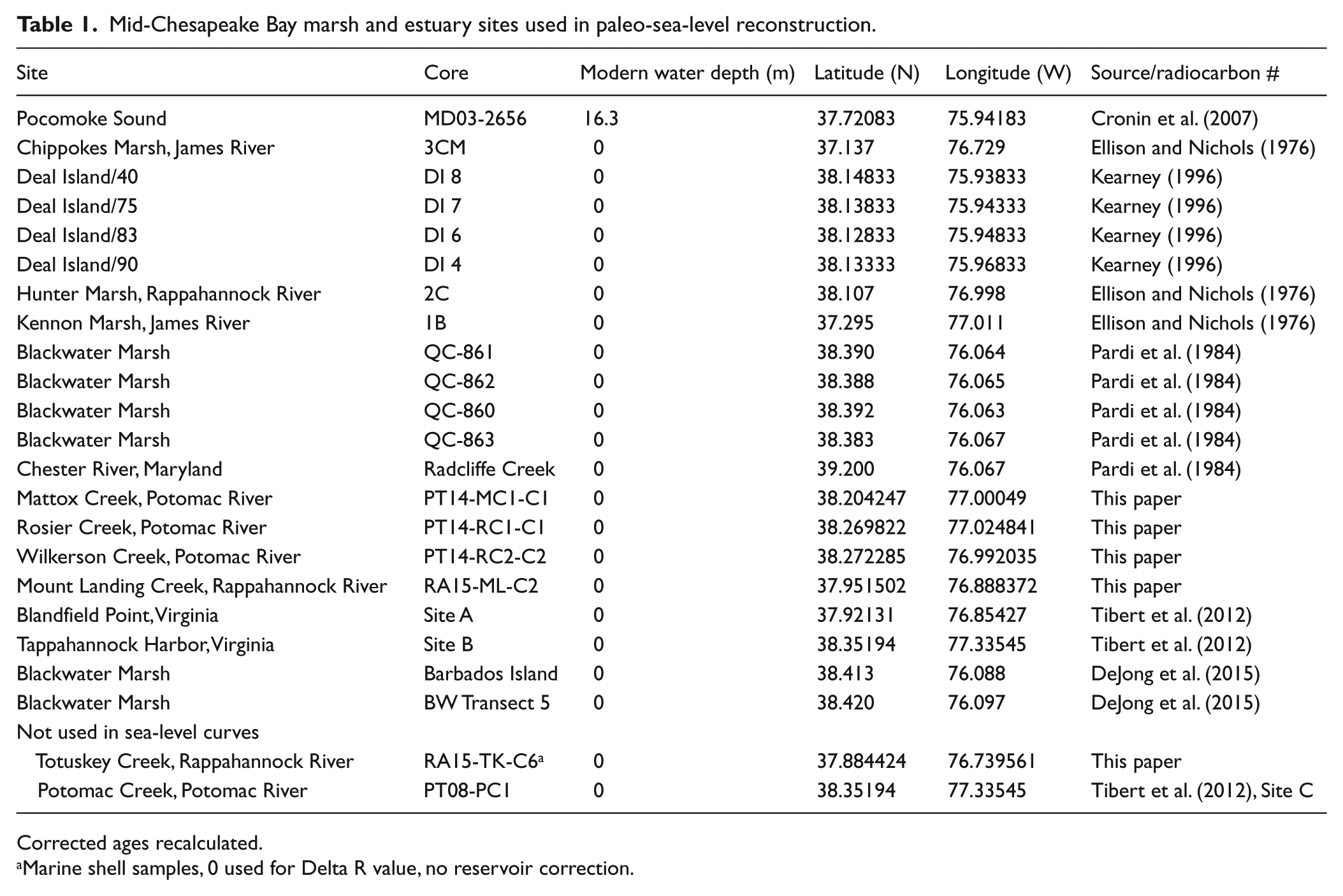
Corrected ages recalculated.

Marine shell samples, 0 used for Delta R value, no reservoir correction.

Figure 1.

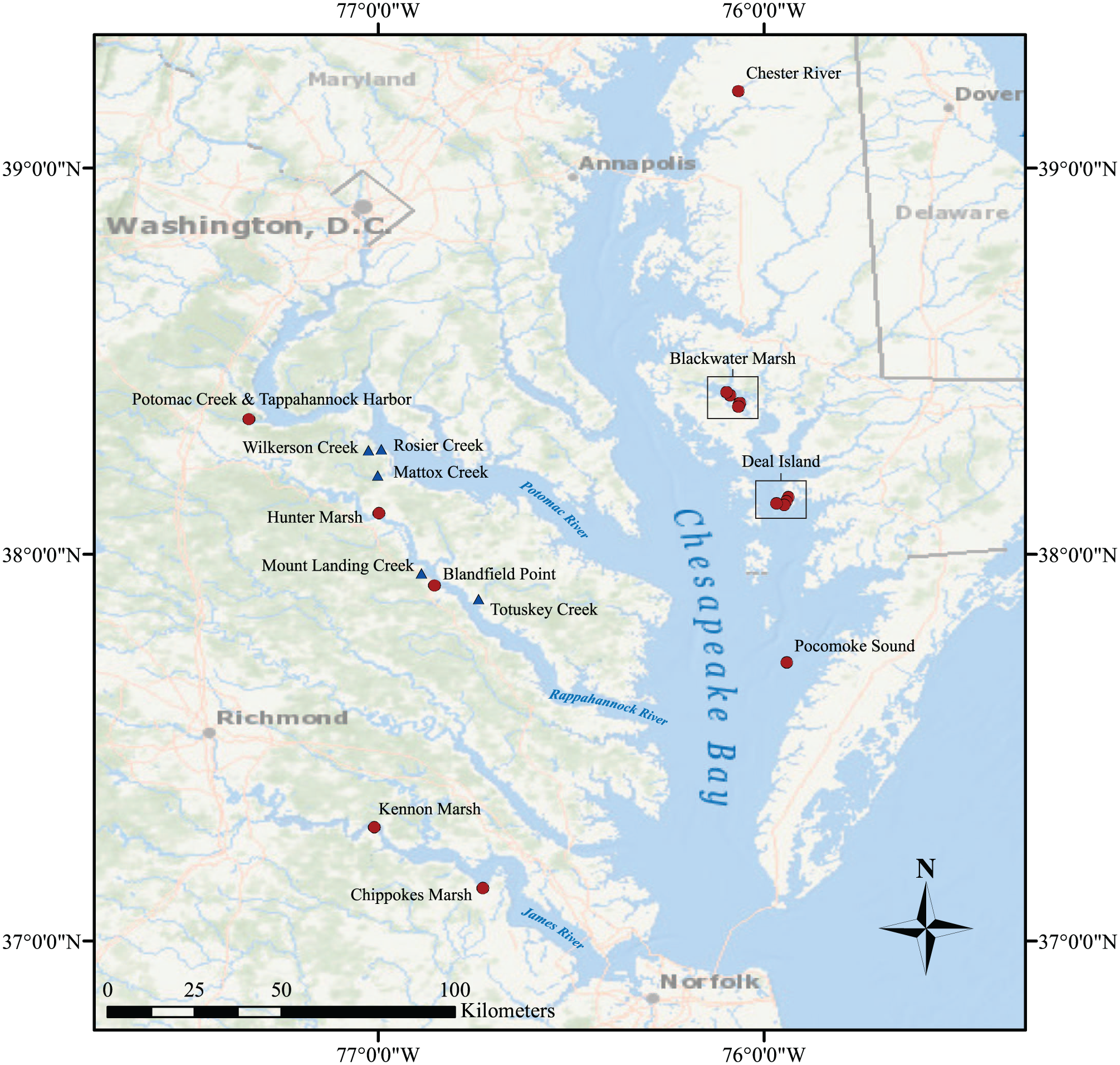
Location maps. Blue triangles are cores focused in the present study. Red circles are other cores from previous studies.

Geochronology

New Accelerator Mass Spectrometry (AMS) ¹⁴C analyses on wood and bulk organic carbon were obtained from the National Ocean Sciences Accelerator Mass Spectrometry (NOSAMS, Woods Hole Oceanographic Institution, MA) and reported in Table 2 along with previously published marsh ages from Chesapeake Bay. Additional dates on fringing reef of Crassostrea virginica from the main channel of the Potomac River are tied to seismic stratigraphy. All dates on peat or peaty organic material, which are used in the current study, were calibrated using Calib 7.10 and the IntCal13 curve (Reimer et al., 2013). Calibrated radiocarbon ages in yr BP (i.e. 1950) were adjusted by adding 64 years to obtain yr BP 2014 (approximate coring year). To obtain an age model for the total organic matter (TOM), MS, and foraminiferal data for each core, we computed using linear sedimentation rates based on the calibrated ¹⁴C dates (Supplemental Appendices 1 and 2, available online). The age model for Totuskey Creek was estimated by matching the TOM and MS figures with those of Mattox, Rosier, Wilkerson, and Mount Landing Creek. Dividing the depth of the core by the age of the AMS ¹⁴C material (Sedimentation Rate = Depth of Core (mm) / ¹⁴C age), Rosier Creek yielded sedimentation rates of about 1.8–2 mm yr⁻¹ for the past 3130 years. Both Wilkerson and Mattox Creeks yielded sedimentation rates of about 1.7–1.8 mm yr⁻¹.

Table 2.

Radiocarbon dates from mid-Chesapeake Bay marshes and estuaries used in paleo-sea-level reconstruction.

Site	Core	Modern water depth (m)	Latitude (N)	Longitude (W)	Source/radiocarbon #	Material dated	Labcode	Sample depth in core (m)	^aMeters BSL	Uncorrected C-14 age	Error	##delta C-13	Calib Median BP 1950	Calib error–	Calib error+	relative area under probability distribution	Calib-Years BP 2014
Chesapeake Bay, south Pocomoke Sound	MD03-2656	16.3	37.72083	75.94183	Cronin et al. (2007)	Plant fronds	211986	5.49	−21.79	7410	40	−12.10	8254	84	87	1.000	8318
Chesapeake Bay, south Pocomoke Sound	MD03-2656	16.3	37.72083	75.94183	Cronin et al. (2007)	Plant material	211981	4.82	−21.12	7210	40	−24.40	8016	61	55	0.802	8080
Chesapeake Bay, south Pocomoke Sound	MD03-2656	16.3	37.72083	75.94183	Cronin et al. (2007)	Plant material	211982	5.02	−21.32	7620	40	−24.60	8414	50	68	0.944	8478
Chesapeake Bay, south Pocomoke Sound	MD03-2656	16.3	37.72083	75.94183	Cronin et al. (2007)	Plant material	211984	5.28	−21.58	7380	30	−14.20	8206	47	115	0.960	8270
Chesapeake Bay, south Pocomoke Sound	MD03-2656	16.3	37.72083	75.94183	Cronin et al. (2007	Plant material	194454	5.80	−22.10	7480	50	−18.60	8300	108	82	1.000	8364
Chesapeake Bay, south Pocomoke Sound	MD03-2656	16.3	37.72083	75.94183	Cronin et al. (2007)	Plant material	OS-40850	6.44	−22.74	8050	50	−26.30	8926	180	164	0.988	8990
Chesapeake Bay, south Pocomoke Sound	MD03-2656	16.3	37.72083	75.94183	Cronin et al. (2007)	Plant material	OS-40851	6.87	−23.17	8290	50	−24.9	9300	172	137	1.000	9364
Chesapeake Bay, south Pocomoke Sound	MD03-2656	16.3	37.72083	75.94183	Cronin et al. (2007)	Plant material	OS-40852	7.31	−23.61	8340	50	−26.3	9360	120	120	0.971	9424
Chesapeake Bay, south Pocomoke Sound	MD03-2656	16.3	37.72083	75.94183	Cronin et al. (2007)	Plant material	180324	7.91	−24.21	8180	50	−17.9	9129	116	146	1.000	9193
Chesapeake Bay, south Pocomoke Sound	MD03-2656	16.3	37.72083	75.94183	Cronin et al. (2007)	Plant material	OS-40853	8.52	−24.82	8270	50	−25.5	9265	151	164	0.985	9329
Chesapeake Bay, south Pocomoke Sound	MD03-2656	16.3	37.72083	75.94183	Cronin et al. (2007)	Plant material	194462	8.98	−25.28	8690	50	−25.2	9641	101	153	0.977	9705
Chesapeake Bay, south Pocomoke Sound	MD03-2656	16.3	37.72083	75.94183	Cronin et al. (2007)	Plant material	194463	9.39	−25.69	8690	50	−24.8	9641	101	153	0.977	9705
Chesapeake Bay, south Pocomoke Sound	MD03-2656	16.3	37.72083	75.94183	Cronin et al. (2007)	Plant material	194464	9.67	−25.97	8580	50	−25.97	9543	61	93	0.967	9607
Chesapeake Bay, south Pocomoke Sound	MD03-2656	16.3	37.72083	75.94183	Cronin et al. (2007)	Plant/seed	OS-40850	6.44	−22.74	7400	50	−26.20	8243	89	109	0.940	8307
Chesapeake Bay, south Pocomoke Sound	MD03-2656	16.3	37.72083	75.94183	Cronin et al. (2007)	Plant/seeds	194455	5.80	−22.10	7780	50	−27.10	8556	128	85	1.000	8620
Chesapeake Bay, south Pocomoke Sound	MD03-2656	16.3	37.72083	75.94183	Cronin et al. (2007)	Plant/wood	211983	5.28	−21.58	7870	40	−28.90	8665	113	117	0.946	8729
Chippokes Marsh, James River	3CM	0	37.137	76.729	Ellison and Nichols (1976)	Basal peat	NA	7.33	−7.33	4880	140	NA	5622	305	291	1.000	5686
Deal Island/40	DI 8	0	38.14833	75.93833	Kearney (1996)	Basal peat	Beta 23320	0.40	−0.40	560	60	NA	588	77	67	1.000	652
Deal Island/75	DI 7	0	38.13833	75.94333	Kearney (1996)	Basal peat	Beta 23319	0.75	−0.75	860	90	NA	790	128	145	1.000	854
Deal Island/83	DI 6	0	38.12833	75.94833	Kearney (1996)	Basal peat	Beta 23318	0.83	−0.83	980	70	NA	878	142	124	0.972	942
Deal Island/90	DI 4	0	38.13333	75.96833	Kearney (1996)	Basal peat	Beta 21803	0.90	−0.90	880	100	NA	809	149	163	1.000	873
Hunter Marsh, Rappahannock River	2C	0	38.107	76.998	Ellison and Nichols (1976)	Basal peat	Geochron Lab # Not Available	0.43	−0.43	980	90	NA	883	184	180	1.000	947
Hunter Marsh, Rappahannock River	5H	0	38.107	76.998	Ellison and Nichols (1976)	Clayey peat	Geochron Lab # Not Available	3.75	−3.75	1570	140	NA	1483	223	335	0.996	1547
Hunter Marsh, Rappahannock River	5H	0	38.107	76.998	Ellison and Nichols (1976)	Basal peat	Geochron Lab # Not Available	5.65	−5.65	2810	160	NA	2958	270	413	0.961	3022
Hunter Marsh, Rappahannock River	3HM	0	38.107	76.998	Ellison and Nichols (1976)	Basal peat	Geochron Lab # Not Available	9.22	−9.22	5780	210	NA	6604	421	557	1.000	6668
Hunter Marsh, Rappahannock River	3E	0	38.107	76.998	Ellison and Nichols (1976)	Clayey peat	Geochron Lab # Not Available	0.3	−0.30	30	60	NA
Hunter Marsh, Rappahannock River	2C	0	38.107	76.998	Ellison and Nichols (1976)	Clayey peat	Geochron Lab # Not Available	0.43	−0.43	320	80	NA	380	112	137	0.919	444
Hunter Marsh, Rappahannock River	3E	0	38.107	76.998	Ellison and Nichols (1976)	Clayey peat	Geochron Lab # Not Available	0.6	−0.60	120	75	NA	140	140	145	1.000	204
Hunter Marsh, Rappahannock River	1B	0	38.107	76.998	Ellison and Nichols (1976)	Basal sandy peat	Geochron Lab # Not Available	0.9	−0.90	535	95	NA	557	129	120	0.951	621
Hunter Marsh, Rappahannock River	3E	0	38.107	76.998	Ellison and Nichols (1976)	Clayey peat	Geochron Lab # Not Available	2.55	−2.55	1260	200	NA	1169	404	384	1.000	1233
Hunter Marsh, Rappahannock River	3HM	0	38.107	76.998	Ellison and Nichols (1976)	Peat	Geochron Lab # Not Available	5.76	−5.76	3310	300	NA	3564	723	734	0.987	3628
Hunter Marsh, Rappahannock River	4g	0	38.107	76.998	Ellison and Nichols (1976)	Peat	Geochron Lab # Not Available	3.85	−3.85	1735	95	NA	1655	179	214	0.949	1719
Hunter Marsh, Rappahannock River	4g	0	38.107	76.998	Ellison and Nichols (1976)	Basal peat	Geochron Lab # Not Available	4.45	−4.45	3345	110	NA	3591	231	276	1.000	3655
Kennon Marsh, James River	1B	0	37.295	77.011	Ellison and Nichols (1976)	Basal peat	Geochron Lab # Not Available	0.90	−0.90	535	95	NA	557	129	120	0.951	621
Kennon Marsh, James River	1KM	0	37.295	77.011	Ellison and Nichols (1976)	Clayey peat	Geochron Lab # Not Available	1.53	−1.53	880	110		811	160	178	0.986	875
Kennon Marsh, James River	2KM	0	37.295	77.011	Ellison and Nichols (1976)	Peat	Geochron Lab # Not Available	3.23	−3.23	1465	110		1381	204	230	1.000	1445
Kennon Marsh, James River	1KM	0	37.295	77.011	Ellison and Nichols (1976)	Basal peat	Geochron Lab # Not Available	2.45	−2.45	1310	160	NA	1215	292	330	1.000	1279
Kennon Marsh, James River	2KM	0	37.295	77.011	Ellison and Nichols (1976)	Basal peat	Geochron Lab # Not Available	4.98	−4.98	2700	160	NA	2822	463	359	0.996	2886
Blackwater Marsh, Maryland	QC-861	0	38.390	76.064	Pardi et al. (1984)	Salt peat	QC-861	−3.64	−3.64	2485	125		2556	249	290	0.994	2620
Blackwater Marsh, Maryland	QC–862	0	38.388	76.065	Pardi et al. (1984)	Salt peat	QC-862	−4.12	−4.12	2650	180		2752	424	462	1.000	2816
Blackwater Marsh, Maryland	QC–860	0	38.392	76.063	Pardi et al. (1984)	Salt peat	QC-860	−3.34	−3.34	2835	140		2983	249	375	1.000	3047
Blackwater Marsh, Maryland	QC–863	0	38.383	76.067	Pardi et al. (1984)	Salt peat	QC-863	−5.57	−5.57	3745	120		4116	292	320	0.986	4180
Chester River, Maryland	Radcliffe Creek	0	39.200	76.067	Pardi et al. (1984)	Salt peat	QC-859	−1.92	−1.92	1230	155		1141	250	271	0.961	1205
Chester River, Maryland	Radcliffe Creek	0	39.200	76.067	Pardi et al. (1984)	Salt peat	QC-857	−5.17	−5.17	3365	145		3621	300	362	0.981	3685
Chester River, Maryland	Radcliffe Creek	0	39.200	76.067	Pardi et al. (1984)	Salt peat	QC-856	−10.87	−10.87	4505	120		5150	297	189	0.893	5214
Mattox Creek	PT14-MC1-C1	0	38.204247	77.00049	This paper	Plant/wood	OS-115289	−0.955	−0.955	115	20		112	93	155	1.000	176
Mattox Creek	PT14-MC1-C3	0	38.204247	77.00049	This paper	Plant/wood	OS-115290	−2.475	−2.475	1700	30	−25.78	1603	59	34	0.755	1667
Mattox Creek	PT14-MC1-C4	0	38.204247	77.00049	This paper	Plant/wood	OS-115763	−3.15	−3.15	2140	20	−21.90	2130	85	27	0.868	2194
Mattox Creek	PT14-MC1-C4	0	38.204247	77.00049	This paper	Plant/wood	OS-115291	−3.805	−3.805	2150	30	−26.50	2144	105	39	0.675	2208
Rosier Creek	PT14-RC1-C1	0	38.269822	77.024841	This paper	Plant/wood	OS-115292	−0.485	−0.485		>Modern	−12.99
Rosier Creek	PT14-RC1-C1	0	38.269822	77.024841	This paper	Plant/wood	OS-115293	−0.775	−0.775		>Modern	−13.12
Rosier Creek	PT14-RC1-C2	0	38.269822	77.024841	This paper	Plant/wood	OS-115300	−1.455	−1.455	265	15	−12.32	304	18	102	0.938	368
Rosier Creek	PT14-RC1-C5	0	38.269822	77.024841	This paper	Plant/wood	OS-115301	−4.075	−4.075	2490	20	−13.66	2583	94	62	0.780	2647
Rosier Creek	PT14-RC1-C6	0	38.269822	77.024841	This paper	Plant/wood	OS-115302	−5.815	−5.815	3030	20	−25.28	3227	61	31	0.765	3291
Rosier Creek	PT14-RC1-C6	0	38.269822	77.024841	This paper	Sediment Org. C	OS-115303	−5.845	−5.845	3130	20	−27.24	3361	32	35	0.836	3425
Wilkerson Creek (RC2)	PT14-RC2-C2	0	38.272285	76.992035	This paper	Plant/wood	OS-115304	−1.315	−1.315	125	20	−28.89	115	103	154	1.000	179
Wilkerson Creek (RC2)	PT14-RC2-C2	0	38.272285	76.992035	This paper	Plant/wood	OS-115305	−1.735	−1.735	495	15	−25.77	524	14	12	1.000	588
Wilkerson Creek (RC2)	PT14-RC2-C2	0	38.272285	76.992035	This paper	Plant/wood	OS-115306	−1.765	−1.765	645	15	−24.76	588	27	8	0.600	652
Wilkerson Creek (RC2)	PT14-RC2-C2	0	38.272285	76.992035	This paper	Plant/wood	OS-115308	−1.815	−1.815	980	15	−26.06	918	14	15	0.724	982
Wilkerson Creek (RC2)	PT14-RC2-C2	0	38.272285	76.992035	This paper	Plant/wood	OS-115307	−1.82	−1.82	665	20	−28.16	644	6	26	0.542	708
Wilkerson Creek (RC2)	PT14-RC2-C2	0	38.272285	76.992035	This paper	Plant/wood	OS-115309	−1.925	−1.925	965	15	−26.00	857	33	10	0.453	921
Wilkerson Creek (RC2)	PT14-RC2-C2	0	38.272285	76.992035	This paper	Plant/wood	OS-115310	−1.93	−1.93	860	20	−25.29	763	37	33	0.980	827
Wilkerson Creek (RC2)	PT14-RC2-C3	0	38.272285	76.992035	This paper	Plant/wood	OS-115312	−2.865	−2.865	1470	20	−25.83	1355	44	37	1.000	1419
Mount Landing Creek	RA15-ML-C2	0	37.951502	76.888372	This paper	Plant/wood	OS-120715	−1.6	−1.6	945	15	−14.78	849	53	26	0.754	913
Mount Landing Creek	RA15-ML-C5	0	37.951502	76.888372	This paper	Plant/wood	OS-120716	−4.03	−4.03	2490	20	−21.79	2583	94	62	0.780	2647
Mount Landing Creek	RA15-ML-C7	0	37.951502	76.888372	This paper	Plant/wood	OS-120743	−7	−7	3650	15	−19.41	3964	60	27	0.853	4028
Mount Landing Creek	RA15-ML-C8	0	37.951502	76.888372	This paper	Plant/wood	OS-120822	−7.53	−7.53	3720	20	−14.09	4042	57	12	0.566	4106
Wilkerson Creek (RC2)	PT14-RC2-C6	0	38.272285	76.992035	This paper	Charcoal	OS-115313	−5.035	−5.035	2490	20	−27.78	2583	94	62	0.780	2647
Blandfield Point, Virginia	Site A	0	37.92131	76.85427	Tibert et al. (2012)	Peat/clay	UCI-37542	−1.32	−1.32	615	20		601	49	12	0.612	665
Blandfield Point, Virginia	Site A	0	37.92131	76.85427	Tibert et al. (2012)	Peat/clay	UCI-37543	−2.31	−2.31	1750	20		1659	55	55	1.000	1723
Blandfield Point, Virginia	Site A	0	37.92131	76.85427	Tibert et al. (2012)	Peat/clay	UCI-37633	−4.56	−4.56	3100	50		3303	127	101	0.984	3367
Tappahannock Harbor, Virginia	Site B	0	37.92131	76.85427	Tibert et al. (2012)	Peat/clay	AA63032	−0.37	−0.37		Modern
Tappahannock Harbor, Virginia	Site B	0	38.35194	77.33545	Tibert et al. (2012)	Peat/clay	AA63037	−1.31	−1.31	851	58	−12.80	771	90	63	0.783	835
Tappahannock Harbor, Virginia	Site B	0	38.35194	77.33545	Tibert et al. (2012)	Peat/clay	AA63033	−2.29	−2.29	1529	41	−23.48	1426	85	101	1.000	1490
Tappahannock Harbor, Virginia	Site B	0	38.35194	77.33545	Tibert et al. (2012)	Clay	AA63035	−4.12	−4.12	2658	43	(–25)	2775	37	77	1.000	2839
Blackwater Marsh, Maryland	Barbados Island	0	38.413	76.088	DeJong et al. (2015)	Plant material	WW6532	−3.70	−0.20	134	35	−12
Blackwater Marsh, Maryland	Barbados Island	0	38.413	76.088	DeJong et al. (2015)	Plant material	WW6533	−3.80	−0.30	863	43	−13.2	775	84	57	0.789	839
Blackwater Marsh, Maryland	Barbados Island	0	38.413	76.088	DeJong et al. (2015)	Plant material	WW6535	−7.80	−4.30	1584	35	−13.6	1471	71	79	1.000	1535
Blackwater Marsh, Maryland	Barbados Island	0	38.413	76.088	DeJong et al. (2015)	Plant material	WW6536	−8.00	−4.50	2087	37	−15.4	2059	91	90	0.984	2123
Blackwater Marsh, Maryland	Barbados Island	0	38.413	76.088	DeJong et al. (2015)	Plant material	WW6537	−8.30	−4.80	1921	36	−18.6	1869	92	80	0.980	1933
Blackwater Marsh, Maryland	BW Transect 5	0	38.420	76.097	DeJong et al. (2015)	Plant material	WW6539	−3.90	0.00	188	34	−12.6	180	180	122	1.000	244
Blackwater Marsh, Maryland^a	BW Transect 5	0	38.420	76.097	DeJong et al. (2015)	Plant material	WW6540^a	−8.40	−8.40	129	34	−23.1
Blackwater Marsh, Maryland	BW Transect 5	0	38.420	76.097	DeJong et al. (2015)	Plant material	WW6541	−8.60	−4.70	4660	40	−26.3	5403	93	70	0.960	5467
Not used
Totuskey Creek	RA15-TK-C6^b	0	37.884424	76.739561	This paper	Mollusc	OS-120782	−5.32	−5.32	1620	20	−5.21	1194	72	63	1.000	1258
Totuskey Creek	RA15-TK-C6^b	0	37.884424	76.739561	This paper	Mollusc	OS-120783	−5.62	−5.62	1610	20	−4.26	1184	81	66	1.000	1248
Totuskey Creek	RA15-TK-C6^b	0	37.884424	76.739561	This paper	Mollusc	OS-120784	−5.86	−5.86	1560	25	−2.69	1121	78	87	1.000	1185
Totuskey Creek	RA15-TK-C9	0	37.884424	76.739561	This paper	Plant/wood	OS-120824	−9.7	−9.7	5110	20	−24.04	5815	60	10	0.560	5879
Wilkerson Creek (RC2)	PT14-RC2-C6^b	0	38.272285	76.992035	This paper	Mollusc	OS-115454	5.005	−5.005	3540	25	−4.47	3423	72	85	1.000	3487
Wilkerson Creek (RC2)	PT14-RC2-C6^b	0	38.272285	76.992035	This paper	Mollusc (C. virg.)	OS-115456	5.015	−5.015	3160	20	−4.90	2944	86	91	1.000	3008
Wilkerson Creek (RC2)	PT14-RC2-C6^b	0	38.272285	76.992035	This paper	Mollusc	OS-115457	5.155	−5.155	3100	20	−3.81	2869	83	78	1.000	2933
Wilkerson Creek (RC2)	PT14-RC2-C6^b	0	38.272285	76.992035	This paper	Mollusc	OS-115458	5.215	−5.215	3470	15	−3.76	3354	62	72	1.000	3418
Wilkerson Creek (RC2)	PT14-RC2-C6^b	0	38.272285	76.992035	This paper	Mollusc	OS-115459	5.215	−5.215	3050	25	−6.22	2811	68	77	1.000	2875
Potomac Creek, Virginia^c	PT08-PC1	0	38.35194	77.33545	Tibert et al. 2012, Site C	Peat/clay	UCI-58708	−0.5	−0.5		Modern
Potomac Creek, Virginia	PT08-PC1	0	38.35194	77.33545	Tibert et al. 2012, Site C	Peat/clay	UCI-58709	−2.63	−2.63	890	20		797	60	6	0.557	861
Potomac Creek, Virginia	PT08-PC1	0	38.35194	77.33545	Tibert et al. 2012, Site C	Clay	UCI-58710	−7.47	−7.47	1855	20		1788	66	45	0.905	1852
Potomac Creek, Virginia	PT08-PC1	0	38.35194	77.33545	Tibert et al. 2012, Site C	Clay	UCI-58739	−7.62	−7.62	2430	25		2456	101	49	0.749	2520

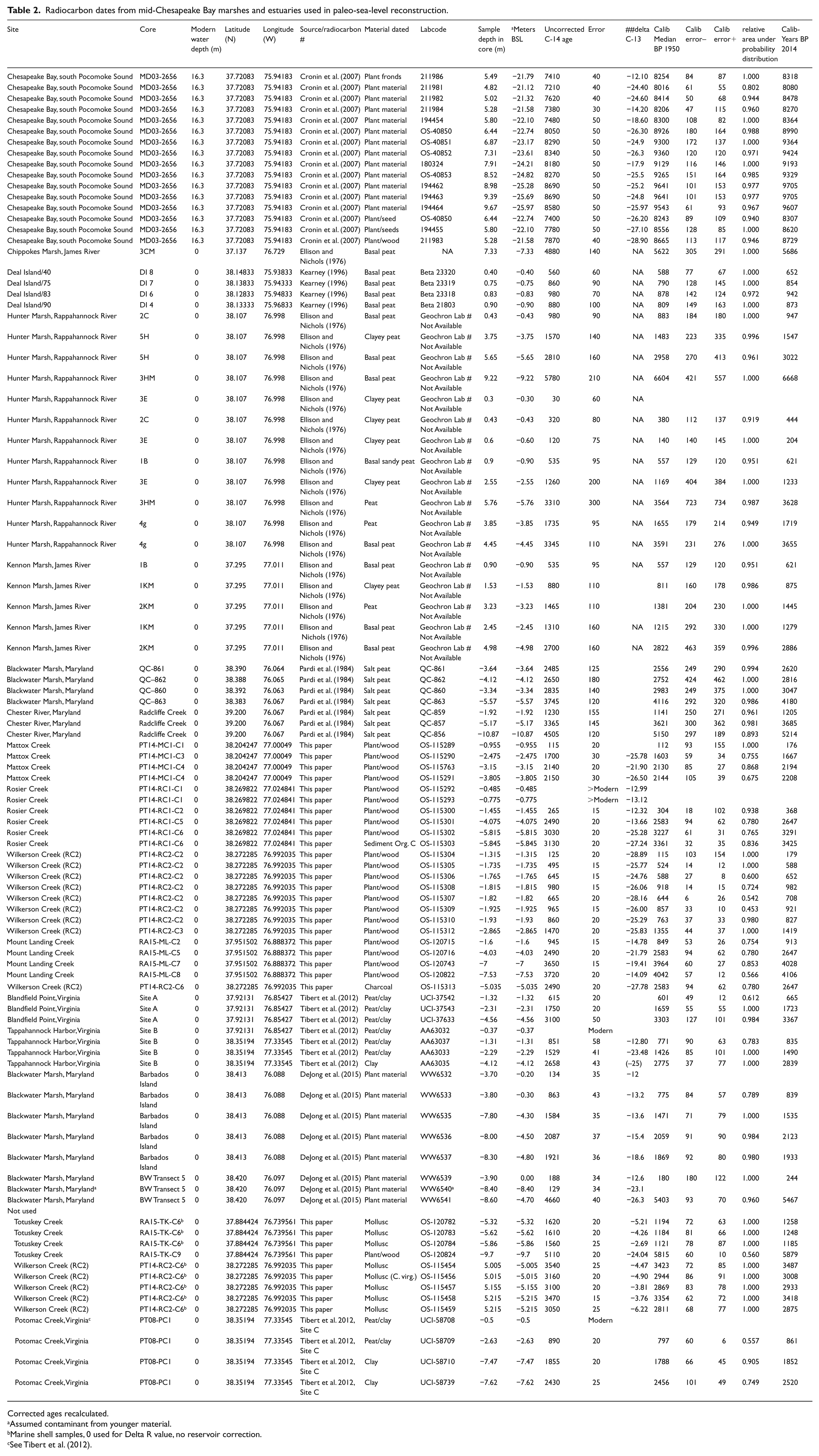
Corrected ages recalculated.

Assumed contaminant from younger material.

Marine shell samples, 0 used for Delta R value, no reservoir correction.

See Tibert et al. (2012).

Results

Physical stratigraphy, MS, and TOM

Cores collected from the Potomac River and Rappahannock River tidal creeks range in length from 5.0 to 6.7 m and the stratigraphy shows two primary lithofacies consisting of a lower, basal gray clay and an upper, organic-rich peat and peaty mud (Figure 2). The gray clay lithofacies has highly variable MS including intensity peaks (~10–20 MS, SI units × 10^–5, Figure 3) and relatively low TOM (4–20%, Figure 4). In contrast, the overlying unit consisting of alternating organic-rich peat and peaty mud has low and relatively invariant MS values (~–5 MS, SI units × 10^–5) and higher TOM (14–82%). Changes in MS are a valuable proxy for environmental changes in estuaries and marshes. Early Holocene tidal marsh sediments recording the first post-glacial SLR into Chesapeake Bay proper have similar lithologies to those in the current study and also had comparable MS values of 10–20 MS, SI units × 10^–5 (Cronin et al., 2007).

Figure 2.

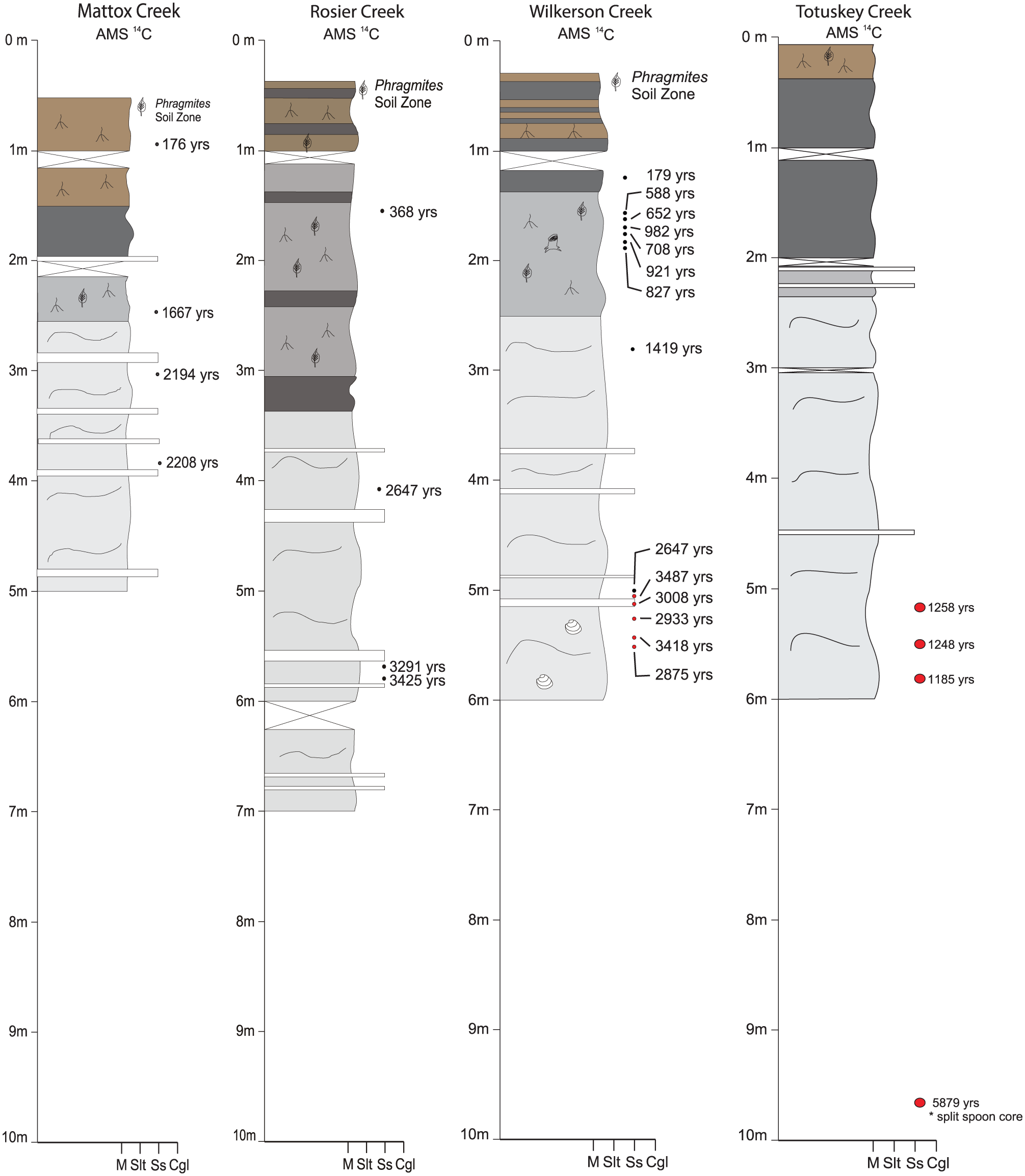
Stratigraphy and location of radiocarbon ages for four cores studied for total organic matter, magnetic susceptibility, and benthic foraminifera. Light gray is estuarine clay facies, darker grays are transition from estuarine to organic-rich marsh peat facies, brown is marsh peat facies. Calibrated radiocarbon ages on plant and organic material are shown for each core (yr BP 2014, see Supplemental Appendix 1, available online). Red circles for Totuskey Creek core are calibrated ages on shells (Crassostrea virginica). See Table 2 for calibrated dates and error uncertainty.

Figure 3.

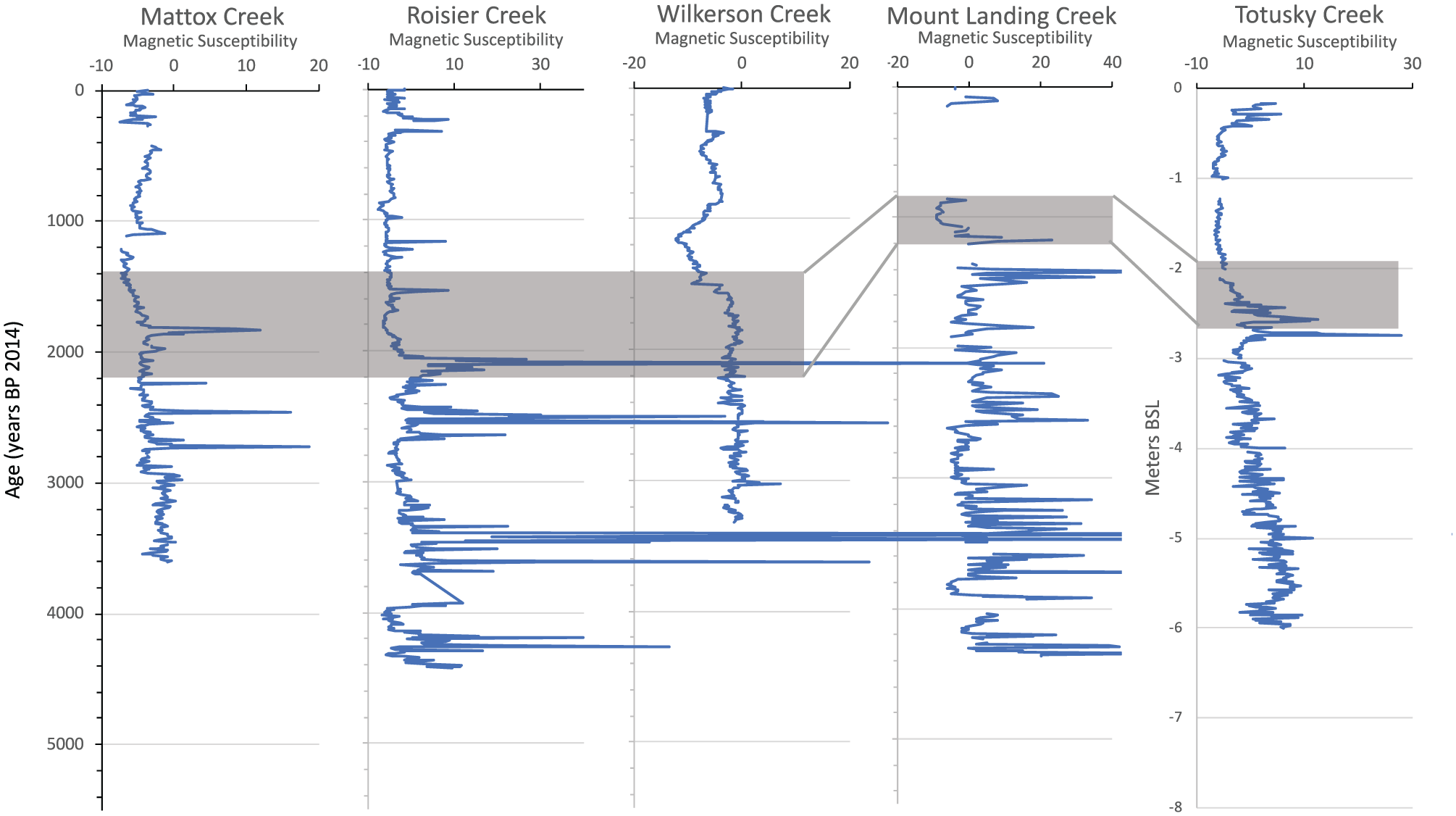
Magnetic susceptibility for five cores. Gray shaded areas approximate transition from clayey estuarine to peat and peaty clay lithofacies.

Figure 4.

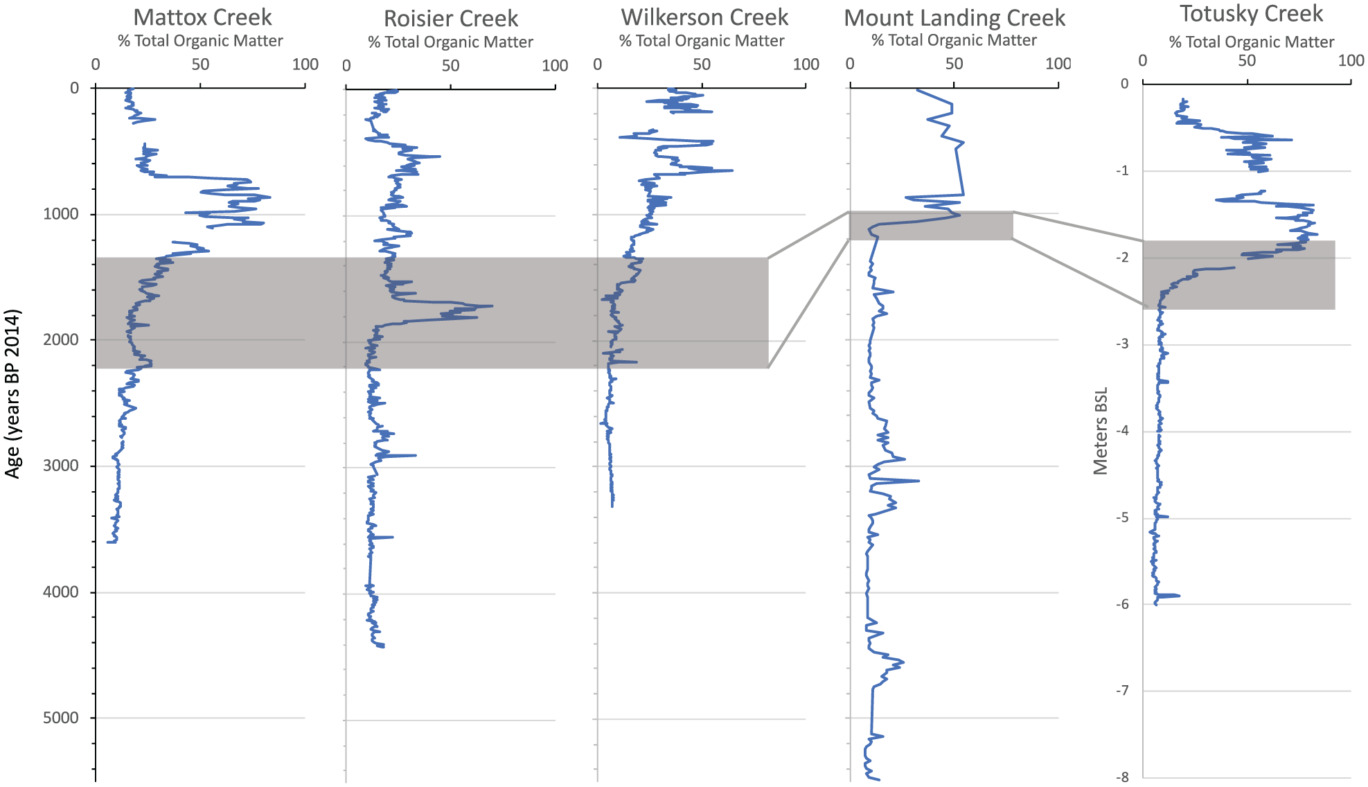
Total organic matter (TOM) based on Loss on Ignition for five marsh cores. Gray shaded areas approximate transition from clayey estuarine to peat and peaty clay lithofacies. Data given in Supplemental Appendix 1, available online.

The clay-to-peat transition in TOM is relatively gradual at the Mattox and Wilkerson sites moderate for the Totuskey Creek site, whereas at Rosier Creek, it is also gradual but interrupted by a peat bed with ~50% TOC dated at ~1800–1600 yr BP. The Mount Landing Creek transition seems to be more abrupt but the age dating is limited at this site. Radiocarbon dates, especially for the better-dated cores (Mattox, Wilkerson), suggest that the transition began about 2000 yr BP and full marsh conditions were reached at about 1000 to 500 yr BP depending on the site (Figure 4). Thus, the peat-forming tidal marsh environment had become predominant in these tributaries before and during the early part of the MCA and, since that time, marsh environments have existed in the study region.

Foraminiferal assemblages

The major foraminiferal assemblages in four cores (Figure 5, Supplemental Appendix 1, available online) contain environmentally diagnostic species well known from eastern US tidal marsh habitats (Culver and Horton, 2005; Ellison and Nichols, 1976; Horton and Culver, 2008; Ishman et al., 1999 and Kemp et al., 2012; Tibert et al., 2012) (see Tibert et al., 2012, for ecology of major taxa). The faunas generally confirm that the clay-to-peat transition represents a shift from deposition in estuarine conditions, dominated by Ammobaculites, which lives at less than one to several meters of water depth (Buzas, 1974; Ellison, 1972), to one of subtidal, intertidal, and high marsh environments (Ammoastuta and other marsh taxa) and even freshwater conditions indicated by abundant thecamoebians at Wilkerson Creek. These marsh biofacies are considered sea-level index points analogous to those used in compilations of Holocene sea-level records along the eastern United States (Engelhart and Horton, 2012, and references therein).

Figure 5.

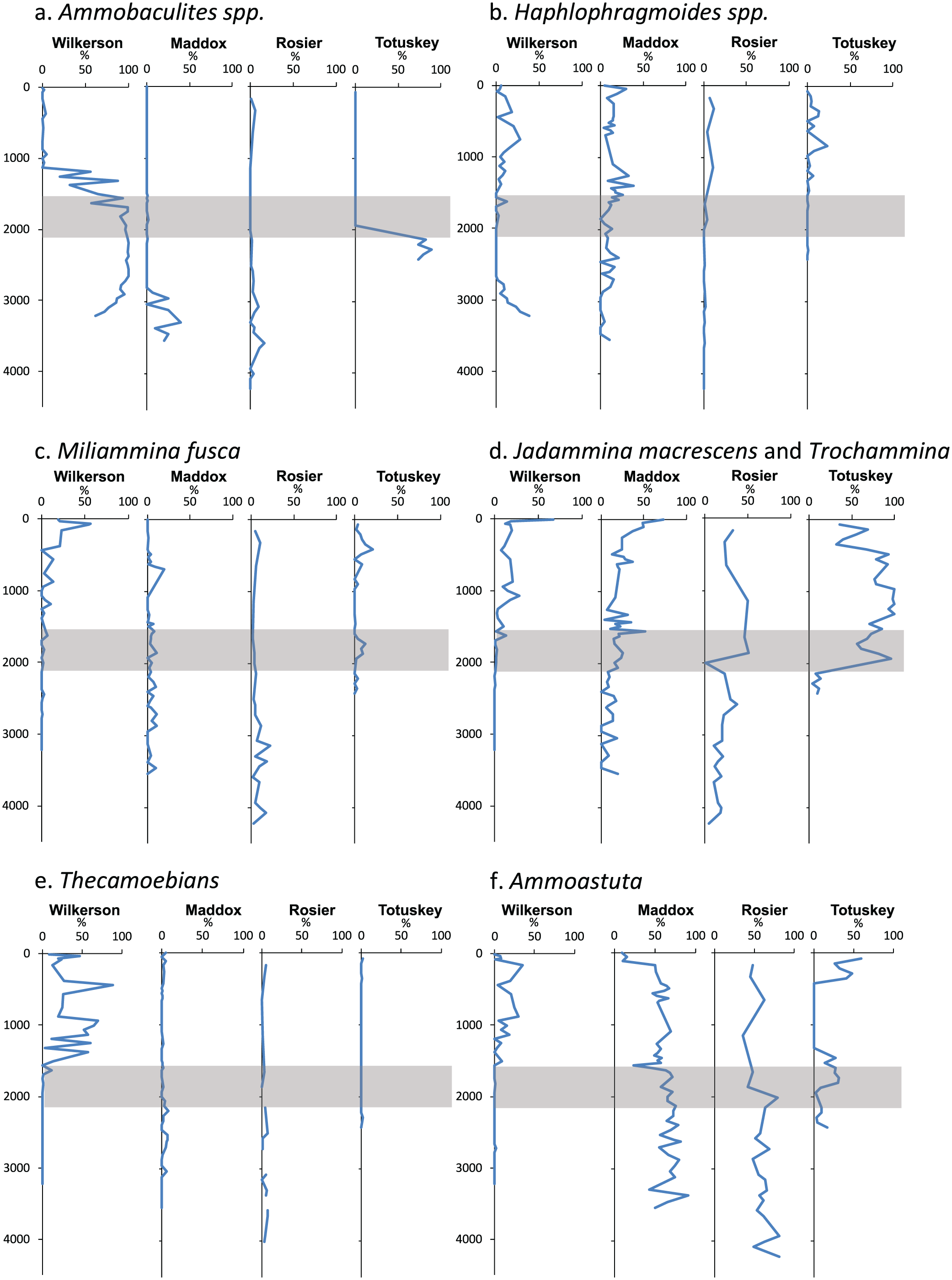
Relative foraminiferal abundances (%) plotted against age (yr BP 2014) for the Wilkerson Creek, Maddox Creek, Rosier Creek, and Totuskey Creek cores. The gray shaded areas represent the time when a transition occurs as seen in the magnetic susceptibility and total organic matter data (Figures 3 and 4). Foraminiferal data are given in Supplemental Appendix 2, available online: (a) Ammobaculites spp., (b) Haplophragmoides spp., (c) Miliammina fusca (d) Jadammina macrescens and Trochammina, (e) Thecamoebians, and (f) Ammoastuta.

In addition to a general transition from estuarine to marsh species, we found that late-Holocene foraminiferal patterns in the Potomac and Rappahannock River marshes vary significantly from site to site. For example, in terms of foraminiferal species dominance, the estuarine to marsh transition is most evident at Wilkerson and Totuskey Creeks, and less obvious at Rosier and Maddox Creeks. These differences reflect different degrees of marsh development due to local conditions in hydrology, salinity, geomorphology, and sedimentology (see Kearney et al., 1994; Ward et al., 1998). Nonetheless, the disappearance of Ammobaculites and the appearance of various combinations of marsh species, as well as the TOM and MS patterns described above, are consistent with the physical stratigraphy (clay-to-peat lithofacies change).

Holocene sea-level curve

Paleo-sea-level reconstructions use radiocarbon ages on plant and organic material and foraminiferal assemblages from tidal marsh deposits to draw relative sea-level curves, although there are many different approaches. First, some studies include ¹⁴C dates on estuarine shells Crassostrea virginica (eastern oyster) or calcareous foraminifera as ‘marine limiting’ dates, which are excellent for giving minimal elevation of a SL datum, but which require a marine reservoir correction and corrections for the dated species’ depth range. Uncertainty in paleo-marsh elevation (PME) of sea-level datums derived from foraminiferal assemblages stems from several sources: infaunal habitat of some foraminiferal species, bioturbation and mixing of sediment, poorly known rates of sediment compaction, changing freshwater and sediment transport to a marsh, and even colonial land use changes since the 18th century.

Second, there are various vertical ecological zonations available for foraminiferal assemblages used to estimate paleo-elevation of a marsh deposit. These typically rely on habitat zonal gradients from offshore to onshore, deeper to shallower, or estuary to high marsh as follows: subtidal estuarine (dates from these deposits are ‘marine limiting’ due to less certainty about water depth), low salt marsh, high salt marsh, and freshwater. Engelhart and Horton (2012) provide a useful schematic diagram (their Figure 1) showing the estimated elevation range that each biofacies indicates relative to mean tide elevation. For example, in the Mid-Atlantic near Atlantic City, New Jersey, low marsh assemblages indicate a height of about 0 to +75 cm a.s.l., high marsh biofacies about +80 to 110 cm a.s.l. In areas like North Carolina, as well as our study region, where tidal ranges are small, the precision of foraminiferal-based paleo-elevations obtained from transfer functions can reach 5–10 cm in well-dated, rapidly accumulating marsh deposits (Kemp et al., 2011).

Most approaches, regardless of salinity, sediment inflow, or plant biology, work on the premise that marshes accrete vertically at or near the rate of SLR, unless this rate exceeds a marshes ability to ‘keep-up’ with rising SL. Our RSL curve shown in Figure 6 shows only peat and organic material ¹⁴C dates and omits dates from mollusks. We plotted the corrected plant and organic material radiocarbon ages from the five new cores along with previously published ages (recalibrated) from Blandfield Point and Rappahannock River, Virginia (Tibert et al., 2012); near Pocomoke Sound, Chesapeake Bay (Cronin et al., 2007); Deal Island, Maryland (Kearney, 1996); Hunter and Kennon Marshes, Virginia (Ellison and Nichols, 1976); Blackwater Marsh and Chester River, Maryland (Pardi et al., 1984); and Blackwater Marsh (DeJong et al., 2015). Core and ¹⁴C age information are given in Tables 1 and 2; locations are plotted in Figure 1.

Figure 6.

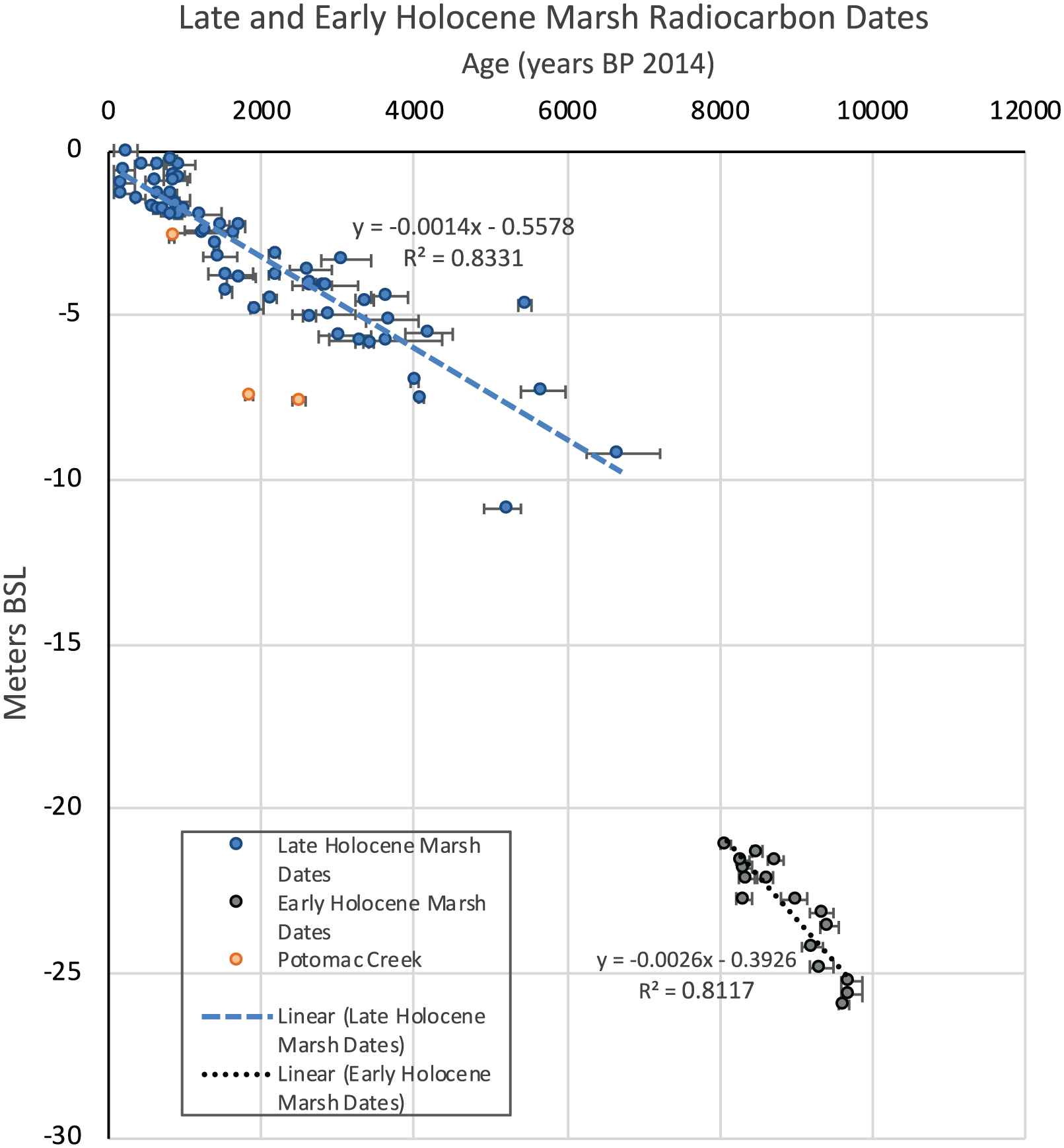
Calibrated ¹⁴C ages versus depth in meters below sea level (MBSL) including only peat, plant, and organic material dates (Table 2). MBSL was calculated by adding the modern water depth to the sample depth in the core. Ages are shown with 2σ error bars and listed as years before present, referring to years before 2014 and were calibrated using Calib 7.10 and the IntCal13 calibration curve (Reimer et al., 2013). Two linear trend lines were calculated based on the radiocarbon dates from all cores except the Potomac Creek core (red circles). The linear trend line for the dates from 11,000 to 8000 yr BP (gray circles) has a slope of 2.6 mm yr⁻¹ while from 6000 to 0 yr BP, the trend line has a slope of 1.4 mm yr⁻¹ (blue circles).

We consider the resulting trend shown in Figure 6 to be a first approximation of centennial-millennial patterns and it is not meant to show multi-decadal RSL changes associated with AMOC variability. We focused on the central part of Chesapeake Bay, where we expect GIA subsidence to be about the same at all sites, and our curve expands substantially on the dataset for region 11 in Chesapeake Bay (Engelhart and Horton, 2012). PMEs were established from the ¹⁴C dates and the stratigraphic distribution of foraminiferal taxa with known vertical ranges in modern salt marshes of the Chesapeake Bay region. Error bars associated with the PMEs are likely small in these microtidal wetlands; however, we do not attempt to be overly precise in using marsh foraminifera as indictors of SL position due to complicating factors: within- and between-marsh differences in hydrology and sediment flow (Kearney and Turner, 2016), storm surges, plant growth and physiology (Kirwan and Megonigal, 2013), sediment compaction (Törnqvist et al., 2008), and infaunal habitats for some species (Culver and Horton, 2005).

Discussion

The overall trends in Figure 6 demonstrate a pattern of rapid early Holocene SLR (10–8 ka) of about 2.6 mm yr⁻¹. This relatively high rate is due to combined final ice-sheet melting at around the time of the 8.2 ka climate event (Cronin et al., 2007) and perhaps a more rapid rate of GIA subsidence (Fletcher, 1988). During the mid to late Holocene, the rate of RSLR was ~1.2 mm yr⁻¹ (6–1 ka) to 1.4 mm yr⁻¹ (6 ka to present). These estimates refine those of earlier studies of GIA subsidence for this region at ~38°N latitude and is consistent with rates of about 1.2–1.5 mm yr⁻¹ in nearby regions of the US Mid-Atlantic region (Engelhart and Horton, 2012; Kopp, 2013; Nikitina et al., 2015).

Estuarine conditions gave way to increased peat production from expanding marsh development prior to and during the MCA and LIA. This shift is pervasive in all aspects of the sediment cores studied. The dominant foraminifera Ammobaculites found in the gray clay lithofacies signifies a period when tidal marshes were absent or poorly developed in this region when the rate of RSLR was 1.2–1.4 mm yr⁻¹. Three intervals (Figure 2, see Table 2) dating the estuarine facies are at Mattox (two dates 2194, 2208 yr BP corrected), Rosier (three dates 2647–3425), and Wilkerson Creek (six dates 2627–3487) sites. Mattox (1667 yr BP) and Wilkerson (1419 yr BP) dates provide an approximate age for the transitional interval. The gradual transition of MS in most cores reach typical values for the peat lithofacies about 1600 to <1000 yr BP (Figure 3). The transition in TOM occurs a little later (Figure 4), depending on the core site. High TOM values characterize the peat lithofacies at all sites, which are best dated at Wilkerson (seven dates, 179–982 yr BP). The general timing of this transition is consistent with ages for an early MCA–LIA transition in Chesapeake Bay temperature (Cronin et al., 2010).

The idea that Holocene SL oscillates in the Mid-Atlantic region is not new. Fletcher et al. (1993) found five transgressive events in Wolfe Glade, Delaware, and other Delaware and New Jersey sites. The youngest boundary was dated at ~1.8 ka. Fletcher dismisses lateral meanders, change in sediment supply, and compaction as an explanation and favors a regional SL Rise, which is consistent with simultaneous drowning of marshes in Connecticut (Varekamp et al., 1992). Re-examining their dates, we estimate that this RSLR before and up to about 1500 yr BP was too rapid for marsh growth, at least in some regions.

Prior studies in the Chesapeake region have also identified a change in the rate of RSLR during the last approximately 1000 years. For example, Kearney (1996) estimated a fall in RSLR rate from 1.6–2.0 mm yr⁻¹ to 0.56 mm yr⁻¹ beginning about 1000 yr BP at Deal Island, Maryland. In addition to Kearney’s (1996) evidence from Deal Island, marsh development was also seen in New Jersey (Varekamp et al., 1992) and North Carolina where RSLR was stable or slightly falling after about 1350 CE (~650 yr BP) (Kemp et al., 2011). In the southeastern United States at the Georgia–Florida border, Kemp et al. (2014) found a low rate of RSLR (0.41 ± 0.08 mm yr⁻¹) prior to 1800 CE). This value is close to the local GIA subsidence rate, and Kemp et al. (2014) assumed no global steric or glacio-eustatic signal in the region. RSL rate slowdown in Guilford, Connecticut (Varekamp and Thomas, 1998; Varekamp et al., 1992) was ~0.3 mm yr⁻¹ about 1200–1600 CE during the LIA.

The change in SLR rate can also be seen in our Figure 7, which suggests a slowdown in the RSLR rate and initiation of marsh accretion occurring about 1500–800 yr BP. The correlation of age to depth of dated interval varies greatly reflecting inter- and intra-marsh differences (e.g. Varekamp and Thomas, 1998), dating uncertainty, and perhaps regional effects of AMOC oscillations during the MCA and the LIA. Such spatial variability is seen in the lithostratigraphy (alterations between peat and clay lithofacies in the uppermost core records (Figure 2) and foraminiferal assemblages (Figure 5). Despite this variability, our estimated post-1000 yr BP RSLR rates are ~0.7 mm yr⁻¹ (r² = 0.84) at Wilkerson Creek and ~0.9 mm yr⁻¹ (r² = 0.92) at Deal Island. Thus, the evidence shows a multi-century shift from a RSLR rate of 1.4 mm yr⁻¹ to about 0.7–0.9 mm yr⁻¹. This suggests that a fall in GMSL of 0.5 to 0.7 mm yr⁻¹ canceled out much of the 1.4 mm yr⁻¹ GIA-induced subsidence.

Figure 7.

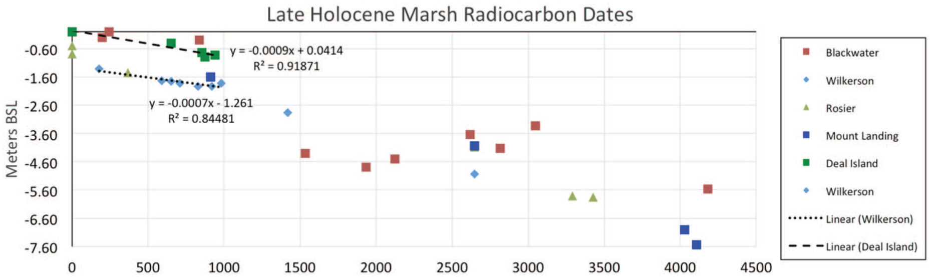
Comparison of dates from last 4500 years (X-axis) for five sites showing a change in RSL rate occurring ~1500–1000 yr BP. The RSLR rates for the last 1000 years for the two well-dated sites are ~0.7 mm yr⁻¹ (r² = 0.84) at Wilkerson Creek and ~0.9 mm yr⁻¹ (r² = 0.92) at Deal Island.

Questions about the relationship between the RSL rate of a particular region and GMSL have confronted the sea-level community for years. How much does GMSL vary during the mid to late Holocene due to thermosteric and glacio-eustatic processes? As a corollary, what was the preindustrial background rate and when did this rate accelerate? Evidence presented here and in previous studies of eastern US marshes suggests that late-Holocene (pre-historical) GMSL fell over the last 1000 years because decreases in regional rates are evident across a large geographical region with very different rates of GIA. Moreover, our new results on the clay–peat transition show this shift was gradual, occurring over centuries. Although a precise rate of falling GMSL cannot be determined due to uncertainty in GIA rates and marsh chronology, it was likely ~0.5–0.7 mm yr⁻¹ and may represent an increase in land ice during the late MCA and LIA. One cannot exclude the possibility that changes in AMOC are also affecting the late-Holocene sea-level patterns although these would be expected over multi-decadal timescales, which probably cannot be detected in most marshes.

Is a glacio-eustatic fall in GMSL a reasonable explanation of marsh sea-level records? There is ample evidence for cooling and advance of alpine and small glaciers during the LIA. Although not synchronous in all regions (Schaefer et al., 2009), LIA cooling and ice advance following the early Holocene thermal maximum is widespread and complex (Briner et al., 2016; Kaufman et al., 2004, 2015; Sundqvist et al., 2014). A similar pattern exists in the late Holocene, pre-anthropogenic cooling in the Arctic (Kaufman et al., 2009; Routson et al., 2019). These qualitative results would imply that background GMSL was falling during the pre-anthropogenic period, at least up until about the year 1800 CE.

If this hypothesis is supported by additional evidence, it leaves us with the dilemma of when GMSL started rising and/or accelerating (Kemp et al., 2009). Rigorous statistical analysis of pre-1990 SLR rates from 622 tide gauges indicate a GMSL rise rate of ~1.2 mm yr⁻¹ up to 1990 (Hay et al., 2015), followed by a faster rate. Geophysical modeling generally confirms this recent acceleration (Mitrovica et al., 2015). These results lead us to conclude that there are at least two recent periods of GMSL rise/acceleration – the first, recognized long ago by Varekamp and Thomas (1998), roughly between ~1800 CE (before the tide gauge record era) and 1900 CE (the beginning of tide gauge records), and a second acceleration from 1.2 to about 3 mm yr⁻¹ since the year 1990 (Hay et al., 2015).

Conclusion

Our results show the highest RSLR rate in the mid-Chesapeake region was 2.6 mm yr⁻¹ during the early Holocene due to a higher rate of GIA and/or glacio-eustatic processes. Although this rate cannot be determined precisely, it was very likely variable during the early Holocene due to changing contributions from glacio-eustatic processes. During the mid to late Holocene, a moderate mean RSLR rate of ~1.2–1.4 mm yr⁻¹ reflects well-constrained GIA subsidence. The RSLR rate from 1000 to 500 yr BP fell to 0.7 to 0.9 mm yr⁻¹, which suggests that a fall in GMSL canceled out part of the GIA subsidence of ~1.4 mm yr⁻¹ in the mid-Atlantic. Thus, between ~1800 and 1900, accelerated GMSL shifted from slow fall to a rise rate of 1.2 mm yr⁻¹.

Supplemental Material

Appendix-2-Tibert-MS-ForamData – Supplemental material for Holocene sea-level variability from Chesapeake Bay Tidal Marshes, USA

Supplemental material, Appendix-2-Tibert-MS-ForamData for Holocene sea-level variability from Chesapeake Bay Tidal Marshes, USA by Thomas M Cronin, Megan K Clevenger, Neil E Tibert, Tammy Prescott, Michael Toomey, J Bradford Hubeny, Mark B Abbott, Julia Seidenstein, Hannah Whitworth, Sam Fisher, Nick Wondolowski and Anna Ruefer in The Holocene

Supplemental Material

Appendix_1-Tibert-TOC-MS – Supplemental material for Holocene sea-level variability from Chesapeake Bay Tidal Marshes, USA

Supplemental material, Appendix_1-Tibert-TOC-MS for Holocene sea-level variability from Chesapeake Bay Tidal Marshes, USA by Thomas M Cronin, Megan K Clevenger, Neil E Tibert, Tammy Prescott, Michael Toomey, J Bradford Hubeny, Mark B Abbott, Julia Seidenstein, Hannah Whitworth, Sam Fisher, Nick Wondolowski and Anna Ruefer in The Holocene

Footnotes

Acknowledgements

Many thanks to faculty, students, and staff of Mary Washington University Department of Earth and Environmental Sciences who assisted the late Dr Neil Tibert in this research and whose theses contain much of the original data. Dr Tibert was the driving force behind this study and he will be missed. Thanks to B DeJong for Blackwater Marsh data, J Kiker for pre-2009 coring data, B Horton for GIA input, and J Wolf, Chesapeake Bay Program for graphics. We thank G L Wingard and an anonymous reviewer for helpful comments. Any use of trade, firm, or product names is for descriptive purposes only and does not imply endorsement by the US Government.

Funding

The author(s) disclosed receipt of the following financial support for the research, authorship, and/or publication of this article: This study was funded by the University of Mary Washington faculty and undergraduate grants (2008–2014) and US Geological Survey Climate R&D Program (2014–2016).

ORCID iD

Thomas M Cronin

Supplemental material

Supplemental material for this article is available online.

References

Barlow

NLM

Shennan

Long

, et al. (2013) Salt marshes as late-Holocene tide gauges. Global and Planetary Change 106: 90–110.

Beckett

Baldwin

Kearney

(2016) Tidal marshes across a Chesapeake Bay subestuary are not keeping up with sea-level rise. PLoS ONE 11(7): e0159753.

Belknap

Kraft

(1977) Holocene relative sea-level changes and coastal stratigraphic units on the northwest flank of the Baltimore Canyon trough geosyncline. Journal of Sedimentary Petrology 47: 610–629.

Bloom

Stuiver

(1963) Submergence of the Connecticut coast. Science 139: 332–334.

Boon

(2012) Evidence of sea level acceleration at U.S. and Canadian tide stations, Atlantic Coast, North America. Journal of Coastal Research 28(6): 1437–1445.

Boon

Brubaker

Forrest

(2010) Chesapeake Bay land subsidence and sea level change: An evaluation of past and present trends and future outlook. A report to the Army Corps of Engineers no. 425, November. Gloucester Point, VA: Virginia Institute of Marine Science.

Bratton

Colman

Thieler

, et al. (2003) Birth of the modern Chesapeake Bay estuary between 7.4 and 8.2 ka and implications for global sea-level rise. Geo-Marine Letters 22: 188–197.

Briner

McKay

Axford

, et al. (2016) Holocene climate change in Arctic Canada and Greenland. Quaternary Science Reviews 147: 340–364.

Buzas

(1974) Vertical distribution of Ammobaculites in the Rhode River, Maryland. Journal of Foraminiferal Research 4(3): 144–147.

10.

Colman

Mixon

(1988) The record of major Quaternary sea-level changes in a large coastal plain estuary, Chesapeake Bay, Eastern United States. Palaeogeography, Palaeoclimatology, Palaeoecology 68: 99–116.

11.

Cronin

(2012) Rapid sea-level rise. Quaternary Science Reviews 56: 11–30.

12.

Cronin

Dwyer

Kamiya

, et al. (2003) Medieval Warm Period, Little Ice Age and 20th century temperature variability from Chesapeake Bay. Global and Planetary Change 36(1–2): 17–29.

13.

Cronin

Farmer

Marzen

, et al. (2014) Late-Holocene sea-level variability and Atlantic Meridional Overturning Circulation. Paleoceanography 29: 765–777.

14.

Cronin

Hayo

Thunell

, et al. (2010) The Medieval Climate Anomaly and Little Ice Age in Chesapeake Bay and the North Atlantic Ocean. Palaeogeography, Palaeoclimatology, Palaeoecology 297: 299–310.

15.

Cronin

Thunell

Dwyer

, et al. (2005) Multiproxy evidence of Holocene climate variability from estuarine sediments. Paleoceanography 20: PA4006.

16.

Cronin

Vogt

Willard

, et al. (2007) Rapid sea level rise and ice sheet response to 8,200-year climate event. Geophysical Research Letters 34: L20603.

17.

Culver

Horton

(2005) Infaunal marsh foraminifera from the Outer Banks, North Carolina, USA. Journal of Foraminiferal Research 35: 148–170.

18.

Davis

Vinogradova

(2017) Causes of accelerating sea level on the East Coast of North America. Geophysical Research Letters 44: 5133–5141.

19.

Dean

Jr (1974) Determination of carbonate and organic matter in calcareous sediments and sedimentary rocks by loss on ignition: Comparison with other methods. Journal of Sedimentary Petrology 44(1): 242–248.

20.

DeJong

Bierman

Newell

, et al. (2015) Pleistocene relative sea levels in the Chesapeake Bay region and their implications for the next century. Geological Society America Today 25(8): 4–10.

21.

Ellison

(1972) Ammobaculites, foraminiferal proprietor of Chesapeake Bay estuaries. Geological Society America Memoir 133: 247–262.

22.

Ellison

Nichols

(1976) Modern and Holocene foraminifera in the Chesapeake Bay region. Maritime Sediments 1: 131–151.

23.

Engelhart

Horton

(2012) Holocene sea level database for the Atlantic coast of the United States. Quaternary Science Reviews 54: 12–25.

24.

Ezer

(2013) Sea level rise, spatially uneven and temporally unsteady: Why the U.S. East Coast, the global tide gauge record, and the global altimeter data show different trends. Geophysical Research Letters 40: 5439–5444.

25.

Ezer

Corlett

(2012) Is sea level rise accelerating in the Chesapeake Bay? A demonstration of a novel new approach for analyzing sea level data. Geophysical Research Letters 39: L19605.

26.

Fletcher

III (1988) Holocene sea level history and neotectonics of the United States Mid-Atlantic region: Applications and corrections. Journal of Geology 96: 323–337.

27.

Fletcher

III Pizzuto

John

, et al. (1993) Sea-level rise acceleration and the drowning of the Delaware coast at 1.8 ka. Geology 21: 121–124.

28.

Haigh

Wahl

Rohling

, et al. (2014) Timescales for detecting a significant acceleration in sea level rise. Nature Communications 5: 3635.

29.

Hay

Morrow

Kopp

, et al. (2015) Probabilistic reanalysis of twentieth-century sea-level rise. Nature 517: 481–484.

30.

Horton

Culver

(2008) Modern intertidal foraminifera of the Outer Banks, North Carolina, U.S.A., and their applicability for sea-level studies. Journal of Coastal Research 24(5): 1110–1125.

31.

Horton

Engelhart

Hill

, et al. (2013) Influence of tidal-range change and sediment compaction on Holocene relative sea-level change in New Jersey, USA. Journal of Quaternary Science 28: 403–411.

32.

Horton

Shennan

Bradley

, et al. (2018) Predicting marsh vulnerability to sea-level rise using Holocene relative sea-level data. Nature Communications 9: 2687.

33.

Ishman

Karlsen

Cronin

(1999) Microfossils from Chesapeake Bay Sediments: Illustrations and Species Database. Open File Report 99-0045. Reston, VA: U.S. Department of the Interior, U.S. Geological Survey.

34.

Karegar

Dixon

Engelhart

(2016) Subsidence along the Atlantic Coast of North America: Insights from GPS and late-Holocene relative sea level data. Geophysical Research Letters 43: 3126–3133.

35.

Kaufman

Ager

Anderson

, et al. (2004) Holocene thermal maximum in the western Arctic (0–180°W). Quaternary Science Reviews 23: 529–560.

36.

Kaufman

Axford

Henderson

ACG

, et al. (2015) Holocene climate changes in eastern Beringia (NW North America) – A systematic review of multi-proxy evidence. Quaternary Science Reviews 147: 312–339.

37.

Kaufman

Schneider

McKay

, et al. (2009) Recent warming reverses long-term Arctic cooling. Science 325: 1236–1239.

38.

Kaye

Barghoorn

(1964) Late quaternary sea-level change and crustal rise at Boston, Massachusetts, with notes on the autocompaction of peat. Bulletin Geological Society of America 75: 63–80.

39.

Kearney

(1996) Sea-level change during the last thousand years in Chesapeake Bay. Journal of Coastal Research 12: 977–983.

40.

Kearney

Turner

(2016) Microtidal marshes: Can these widespread and fragile marshes survive increasing climate–sea level variability and human action? Journal of Coastal Research 32(3): 686–699.

41.

Kearney

Stevenson

Ward

(1994) Spatial and temporal changes in marsh vertical accretion rates at Monie Bay: Implications for sea-level rise. Journal of Coastal Research 10: 1010–1020.

42.

Kemp

Horton

Culver

, et al. (2009) Timing and magnitude of recent accelerated sea-level rise (North Carolina, United States). Geology 37(11): 1035–1038.

43.

Kemp

Horton

Donnelly

, et al. (2011) Climate related sea-level variations over the past two millennia. Proceedings of the National Academy of Sciences 108: 11017–11022.

44.

Kemp

Horton

Vane

, et al. (2014) Sea-level change during the last 2500 years in New Jersey, USA. Quaternary Science Reviews 81: 90–104.

45.

Kemp

Horton

Vann

, et al. (2012) Quantitative vertical zonation of salt-marsh foraminifera for reconstructing former sea level: An example from New Jersey, USA. Quaternary Science Reviews 54: 26–39.

46.

Kemp

Kegel

Culver

, et al. (2017) Extended late-Holocene relative sea-level histories for North Carolina, USA. Quaternary Science Reviews 160: 13–30.

47.

Kirwan

Megonigal

(2013) Tidal wetland stability in the face of human impacts and sea-level rise. Nature 504: 53–60.

48.

Kirwan

Temmerman

Skeehan

, et al. (2016) Overestimation of marsh vulnerability to sea level rise. Nature Climate Change 6: 253–260.

49.

Kopp

(2013) Does the mid-Atlantic United States sea level acceleration hot spot reflect ocean dynamic variability? Geophysical Research Letters 40: 3981–3985.

50.

Kopp

Kemp

Bittermann

, et al. (2016) Temperature-driven global sea-level variability in the Common Era. Proceedings of the National Academy of Sciences of the United States of America 113(11): E1434–E1441.

51.

Lentz

Thieler

Plant

, et al. (2016) Evaluation of dynamic coastal response to sea-level rise modifies inundation likelihood. Nature Climate Change 6: 696–700.

52.

Long

Barlow

NLM

Gehrels

, et al. (2014) Contrasting records of sea-level change in the eastern and western North Atlantic during the last 300 years. Earth and Planetary Science Letters 388: 110–122.

53.

Lyu

Zhang

Church

, et al. (2014) Time of emergence for regional sea-level change. Nature Climate Change 4: 1006–1010.

54.

Milliman

Emery

(1968) Sea-levels during the past 35,000 years. Science 162: 1121–1123.

55.

Mitchell

Herman

Bilkovic

, et al. (2017) Marsh persistence under sea-level rise is controlled by multiple, geologically variable stressors. Ecosystem Health and Sustainability 3(10): 1379888.

56.

Mitrovica

Hay

Morrow

, et al. (2015) Reconciling past changes in Earth’s rotation with 20th century global sea-level rise: Resolving Munk’s enigma. Science Advances 1: e1500679.

57.

National Oceanic and Atmospheric Administration (NOAA) (2015) Mean sea level trends for stations in Virginia. Tides and Currents. Available at: http://tidesandcurrents.noaa.gov/sltrends/sltrends.html.

58.

Nerem

Beckley

Fasullo

, et al. (2018) Climate-change–driven accelerated sea-level rise detected in the altimeter era. Proceedings of the National Academy of Sciences of the United States of America 115: 2022–2025.

59.

Nicholls

Cazenave

(2010) Sea-level rise and its impact on coastal zones. Science 328: 1517–1520.

60.

Nikitina

Kemp

Engelhart

, et al. (2015) Sea-level change and subsidence in the Delaware Estuary during the last~2200 years. Estuarine, Coastal and Shelf Science 164: 506–519.

61.

Nowaczyk

(2001) Logging of magnetic susceptibility. In: Last

Smol

(eds) Tracking Environmental Change Using Lake Sediments: Basin Analysis, Coring, and Chronological Techniques, vol. 1. Dordrecht: Kluwer Academic Publishers, pp.155–170.

62.

Pardi

Tomecek

Newman

(1984) Queens College radiocarbon measurements IV. Radiocarbon 26: 412–430.

63.

Parkinson

Craft

DeLaune

, et al. (2017) Marsh vulnerability to sea-level rise. Nature Climate Change 7: 755.

64.

Peltier

Argus

Drummond

(2015) Space geodesy constrains ice age terminal deglaciation: The global ICE-6G_C (VM5a) model. Journal of Geophysical Research: Solid Earth 120: 450–487.

65.

Pope

Burbey

(2004) Multiple-aquifer characterization from single borehole extensometer records. Ground Water 42: 45–58.

66.

Reed

(1995) The response of coastal marshes to sea-level rise: Survival or submergence. Earth Surface Processes and Landforms 20: 39–48.

67.

Reimer

Bard

Bayliss

, et al (2013) IntCal 13 and Marine13 radiocarbon age calibration curves 0-50,000 years cal BP. Radiocarbon 55: 1869–1887.

68.

Routson

McKay

Kaufman

, et al. (2019) Mid-latitude net precipitation decreased with Arctic warming during the Holocene. Nature 568: 83–87.

69.

Schaefer

Denton

Kaplan

, et al. (2009) High-frequency Holocene glacier fluctuations in New Zealand differ from the northern signature. Science 234: 622–625.

70.

Scholl

(1964) Recent sedimentary record in mangrove swamps and rise in sea level over the southwestern coast of Florida: Part 1. Marine Geology 1: 344–366.

71.

Scholl

Stuiver

(1967) Recent submergence of southern Florida: A comparison with adjacent coasts. Bulletin Geological Society of America 78: 437–454.

72.

Slangen

ABA

Church

Agosta

, et al. (2016) Anthropogenic forcing dominates global mean sea-level rise since 1970. Nature Climate Change 6: 701–706.

73.

Sundqvist

Kaufman

McKay

, et al. (2014) Arctic Holocene proxy climate database – New approaches to assessing geochronological accuracy and encoding climate variables. Climate of the Past Discussions 10: 1605–1631.

74.

Thompson

Hamlington

Landerer

, et al. (2016) Are long tide gauge records in the wrong place to measure global mean sea level rise? Geophysical Research Letters 43: 10403–10411.

75.

Tibert

Hubeny

Abbott

, et al. (2012) Late Holocene sedimentation and paleoenvironmental history for the Tidal Marshes of the Potomac and Rappahannock Rivers, Tributaries, and the Chesapeake Bay. Virginia Journal of Science 63(3–4): 91–109.

76.

Törnqvist

Wallace

Storms

, et al. (2008) Mississippi Delta subsidence primarily caused by compaction of Holocene strata. Nature Geoscience 1(3): 173–176.

77.

Varekamp

Thomas

(1998) Climate change and the rise and fall of sea level over the millennium. Eos Transactions American Geophysical Union 79(6): 69.

78.

Varekamp

Thomas

Van de Plassche

(1992) Relative sea-level rise and climate change over the last 1500 years. Terra Nova 4: 293–304.

79.

Ward

Kearney

Stevenson

(1998) Variations in sedimentary environments and accretionary processes in estuarine marshes undergoing rapid submergence, Chesapeake Bay. Marine Geology 151: 111–134.

80.

Willard

Cronin

Verardo

(2003) Late-Holocene climate and ecosystem history from Chesapeake Bay sediment cores, USA. The Holocene 13(2): 201–214.

Supplementary Material

Please find the following supplemental material available below.

For Open Access articles published under a Creative Commons License, all supplemental material carries the same license as the article it is associated with.

For non-Open Access articles published, all supplemental material carries a non-exclusive license, and permission requests for re-use of supplemental material or any part of supplemental material shall be sent directly to the copyright owner as specified in the copyright notice associated with the article.

0.00 MB

0.03 MB

0.39 MB