Placing the AD 2014–2016 ‘protracted’ El Niño episode into a long-term context

Introduction

The El Niño–Southern Oscillation (ENSO) phenomenon is manifest by many physical forms, encompassing a family of events and episodes which, individually, can vary in their onset, duration, strength, decay, spatial structure across the Indo-Pacific region and teleconnections to higher latitudes in both hemispheres (e.g. Allan, 2000; Capotondi et al., 2015; Johnson, 2013; Lyu et al., 2017; Neelin et al., 1998; Newman et al., 2011; Philander, 1990; Santoso et al., 2019; Timmermann et al., 2018; Wang et al., 2017). There is also strong evidence that ENSO has waxed and waned historically, including multidecadal epochs when it has been more coherent and spatially extensive, with pronounced El Niño and La Niña events, episodes and teleconnections, juxtaposed with epochs when it has contracted spatially and displayed less distinct El Niño and La Niña signatures, episodes and regional teleconnections (e.g. Allan, 2000; Allan et al., 1996; Brown, 2014; Hope et al., 2017). Furthermore, this is occurring within an envelope of multidecadal to centennial scale fluctuations in the global climate system (e.g. Allan, 2000; Allan et al., 1996; Chang et al., 2014; Zanchettin et al., 2010). As a consequence, although El Niño and La Niña events produce more or less opposite impacts across and around the Indo-Pacific basin, no two events are exactly the same.

Over the last 10–20 years, interest in low-frequency ‘ENSO-like’ modes and their teleconnections and impacts has grown to rival that of the more ‘classical’ interannual signature of ENSO centering around the 2–7 or so year timescale (e.g. Capotondi et al., 2015; Hope et al., 2017; Lyu et al., 2017; Meinke et al., 2005; Santoso et al., 2019; Wang et al., 2017). However, there has also been considerable debate as to whether these modes, such as the Interdecadal Pacific Oscillation (IPO)/Pacific Decadal Oscillation (PDO) and similar such modes, are distinct physical entities (Newman et al., 2018). As Wang et al. (2017: 97) note, ‘. . . analysis techniques that pre-suppose a particular timescale through band-pass or low-pass filtering may not be isolating any underlying physical phenomenon but simply sampling a continuum of low-frequency variability, albeit with a well-defined geographical pattern’. There has also been the suggestion that studies should look to isolate and remove the ENSO signal, or at least the interannual ENSO component, in the first instance and then analyse what remains (Compo and Sardeshmukh, 2010).

Among the efforts to better understand ENSO’s nature and characteristics have been studies that have reported different ‘flavours’ of ENSO in the Pacific Ocean basin, as recently reviewed by Capotondi et al. (2015) and Santoso et al. (2019). Most notable is the resolution of distinct Central Pacific (CP) and Eastern Pacific (EP) types (see Figure 1), the culmination of work on the Trans-Niño Index (TNI) (Trenberth and Stepaniak, 2001), Date Line El Niño (Larkin and Harrison, 2005), El Niño Modoki (Ashok et al., 2007), Warm Pool El Niño (Kug et al., 2009) and a number of others (see Capotondi et al. 2015). Interestingly, the CP ENSO type structurally maps closely to the patterns of a quasi-decadal signal in the Pacific Ocean exhibiting ENSO characteristics, first designated by Allan and D’Arrigo (1999) as occurring during ‘protracted’ El Niño and La Niña episodes.

OPEN IN VIEWER

Figure 1.

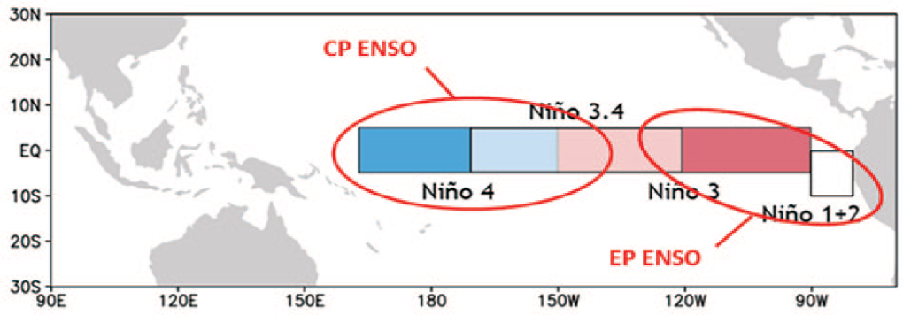
Central Pacific (CP) and Eastern Pacific (EP) types in relation to the spatial dimensions of the Niño 1+2, 3, 3.4 and 4 SST anomaly regions across the tropical Pacific.

These extended ENSO episodes have been defined and redefined, from the historical instrumental data as,

. . . periods of 24 months or more when the SOI [Southern Oscillation Index] and the Niño 3 and 4 CEP-EEP SST [Central Equatorial-Eastern Equatorial Pacific Sea Surface Temperature] indices were of persistently negative or positive sign, or of the opposite sign in a maximum of only two consecutive months during the period . . . (Allan and D’Arrigo, 1999)

This definition was used because, as well as ‘classical’ events that usually lasted for around 9–12 months, sometimes 18 months, there were longer episodes which lingered for a number of years. These were defined as ‘protracted’ episodes when they were of 2 years and more duration. Palaeoclimatic episodes were defined as persisting for 3 years or more in the Stahle et al. (1998) SOI and Niño 3.4 SSTs represented by the Coupled ENSO Index (CEI) used by Gergis and Fowler (2005, 2009). The 3-year definition necessarily takes into account the (varying) degree of autocorrelation inherent in palaeoclimate reconstructions, and their difference in resolution (typically lower) from the instrumental record.

Thus, here, we propose the definition of a ‘protracted’ episode as occurring when the SOI and Niño 4 SST anomalies are of either sign for 2 years or more, with any sign change in that period being in a maximum of only two consecutive months, when using instrumental records, and 3 years or more when analysing palaeoclimatic ENSO reconstructions (Allan and D’Arrigo, 1999; Gergis and Fowler, 2009). For further information on the sensitivity of the protracted ENSO definitions using instrumental and palaeoclimate data, the reader is referred to the original publications of Allan and D’Arrigo (1999) and Gergis and Fowler (2005, 2009) where these assessments are detailed. We also use the term episodes rather than events to define such El Niño and La Niña types, because they last longer than ‘classical’ ENSO events, and display a waxing and waning or ‘sawtooth’ nature of the atmospheric and oceanic variable (e.g. mean sea level pressure (MSLP), SST and sea level) responses defining them during their evolution and duration (see section ‘Overview of the dynamical causes of “Protracted” ENSO episodes’).

The nature and severity of the prolonged 2014–2016 El Niño in the western Pacific has prompted renewed interest in attempting to characterise the long-term context of ENSO extremes. To help with this effort, here, we provide a systematic review of the literature to provide insight into the dynamical characteristics of extended ENSO episodes and a preliminary investigation of their long-term behaviour. Our intention is to not provide an exhaustive analysis testing all the conceptual elements considered here, instead we aim to provide a first consolidation of the relevant literature and provide a ‘proof of concept’ guide for future research. We begin by revisiting evidence of ‘protracted’ ENSO episodes in instrumental data and palaeoclimatic reconstructions. We then review the possible mechanisms underlying such episodes, and look to place the 2014–2016 ‘protracted’ El Niño into a historical context. Finally, we suggest that improved knowledge and the potential to forecast such episodes would be of immense benefit to communities most affected by severe impacts of ENSO extremes, particularly in regions like eastern Australia (Murphy and Ribbe, 2004).

Data and method

Overview of the dynamical causes of ‘protracted’ ENSO episodes

Before presenting a new analysis of protracted ENSO episodes back to 1300, first we begin with a review of the dynamical mechanisms associated with this aspect of ENSO behaviour. In Allan (2000), a joint Multi-Taper Method–Singular Value Decomposition (MTM-SVD) multivariate signal analysis of global MSLP and SST was used to resolve the spectral characteristics of ENSO. Of the significant peak spectral features identified, it was suggested in Allan and D’Arrigo (1999) and Allan et al. (2003) that when the interplay between the quasi-biennial oscillation (QBO), ‘classical’ interannual (LF) and quasi-decadal oscillation (QDO) ENSO signals is dominated by the QDO signal, this leads to the formation of ‘protracted’ El Niño and La Niña episodes. The latter of these signals displays a distinct CP SST pattern, as seen in Figure 2a–c.

OPEN IN VIEWER

Figure 2.

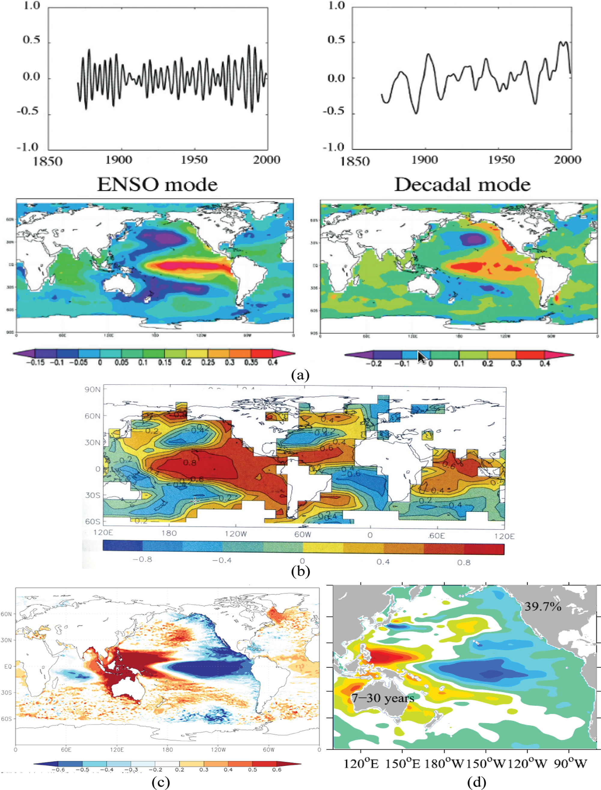
(a) The two leading modes of Niño 4 SST anomalies extracted through singular spectrum analysis. The upper panels represent the reconstruction of the Niño 4 SST anomaly index using the two leading modes (20% of variance for ENSO mode and 25% for decadal mode), units are in K. The lower panels represent the regression patterns of SST anomalies using the upper two timeseries as indices, units are in K/standard deviation (courtesy of Mojib Latif) (source: Wang and Picaut, 2004). (b) Global Sea Ice and Sea Surface Temperature (GISST) 3.0 EOF1 spatial correlation fields for 1871–1994 global SST (relative to the base period 1901–1990) in the 11- to 13-year band (explaining 25.4% of the variance) using a joint Global Mean Sea Level Pressure (GMSLP) 2.1f and GISST3.0 EOF1 timeseries. Correlation values are shown in the bar below the panel (source: Allan, 2000). Regions where <40% of the observations occur are masked (source: Allan, 2000). (c) LHS: Correlations between the Southern Oscillation Index and Copernicus 1/4° 1993–2018 global sea level anomalies. Correlation values are shown in the bar below the panel (source: https://cds.climate.copernicus.eu/cdsapp#!/dataset/satellite-sea-level-global?tab=overview) and RHS: EOF1 patterns of sea level variations (cm) in the Pacific on timescales. (d) Between 7- and 30-year steric sea level in the 1945–2010 period. The percentage represents the amount of variance explained by the EOF1 (source: Lyu et al., 2017).

A number of studies have isolated the existence of quasi-decadal ‘ENSO-like’ signals in variables such as SST, sea level and combined SST and MSLP modes centering on the western equatorial Pacific (e.g. Allan, 2000; Lyu et al., 2017; Wang and Picaut, 2004). These spatial signals, with prominent ‘ENSO-like’ quasi-decadal characteristics, are distinct from those of even lower frequency associated with the IPO/PDO phenomenon. They can be seen using a mix of different observational datasets of varying temporal extents, and resolved by various signal-processing techniques, as seen in Figure 2. This would suggest the operation of similar dynamical mechanisms underlying these QDO ENSO-like features of the ocean–atmosphere system in the Indo-Pacific domain.

There are a number of theories that have been proposed to explain the mechanisms and ocean–atmosphere processes underlying ENSO dynamics that have relevance for understanding the potential causes of protracted episodes. Most recently, these have been reviewed by Capotondi et al. (2015), Wang et al. (2017) and Timmermann et al. (2018). When addressing the nature of the different ‘flavours’ of ENSO in the Pacific Ocean basin, they detail the various dynamical mechanisms put forward to explain them – principally being the delayed oscillator (e.g. Battisti and Hirst, 1989; Cane et al., 1990; Graham and White, 1988; Suarez and Schopf, 1988), the recharge oscillator (Jin, 1997), the western Pacific oscillator (Wang et al., 1999; Weisberg and Wang, 1997), unified oscillator (Wang, 2001) and the advective-reflective oscillator (Picaut et al., 1997), or ‘. . . that disturbances external to the coupled system are the source of random forcing that drives ENSO’ (Wang et al., 2017: 90). Most of these oscillators involve interactions between oceanic equatorial and off-equatorial Rossby and ‘equatorially trapped’ Kelvin Waves of upwelling or downwelling form, and their reshaping, chanelling and trapping as a result of the geography and bathymetry of the Pacific basin.

It was during the early course of discussions about the above ENSO mechanisms that Allan and D’Arrigo (1999) and Allan et al. (2003) first saw patterns in Pacific Niño 4 SST anomalies peaking on decadal timescales that occurred during periods where the interplay between the varying phases of the QDO, ‘classical’ (LF) interannual and QBO ENSO signals, which dictate the multi-temporal nature of the ENSO phenomenon, were dominated by the QDO ENSO signal (Figure 4, in Suarez and Schopf, 1988). This interplay of signals also appeared to give rise to the waxing and waning or ‘sawtooth’ nature of the atmospheric and oceanic variable (e.g. MSLP, SST and sea level) responses during ‘protracted’ episodes of both El Niño and La Niña type detailed in Allan and D’Arrigo (1999) and Allan et al. (2003). Episodes could appear to be terminating, only to become coherent and pronounced again, during the course of their evolution and duration – hence, the use of the distinct term ‘episodes’ to define these El Niño and La Niña types rather than events.

Papers such as White et al. (2003) and White and Tourre (2007) provided schematic representations of the pattern of equatorial and off-equatorial Kelvin and Rossby waves and ocean dynamics that they postulated were at the heart of the delayed action oscillator (DAO) mechanism underlying ‘classical’ and quasi-decadal ENSO modes in the wider Indo-Pacific domain (see Figure 3). The dynamical interactions and patterns displayed with this wider geographical focus are also consistent with the SST responses in Figure 2a–c, with highest tropical Pacific SST anomalies concentrated in the Niño 4 region in ‘protracted’ ENSO episodes and in the Niño 3 to 3.4 regions during ‘classical’ ENSO events (see their evolution in Figure 3). Thus, both ‘classical’ ENSO events and ‘protracted’ ENSO episodes have variants of a common driving mechanism, which is not seen in the above analyses with low-frequency ‘ENSO-like’ phenomena, such as the IPO/PDO (e.g. Battisti and Hirst, 1989; Suarez and Schopf, 1988). This example illustrates the importance of employing sophisticated approaches to resolving and isolating the full ENSO signal and its phasing from the background climate system, as shown in Compo and Sardeshmukh (2010).

OPEN IN VIEWER

Figure 3.

Spatio-temporal evolution of the interdecadal signal (I) (left column), decadal signal (D) (middle left column), ENSO signal (E) (middle right column) and biennial signal (B) (right column) resolved in a Multi-Taper Method/Singular Value Decomposition (MTM/SVD) technique with three tapers of joint sea surface temperature (SST) and sea level pressure (SLP) gridded datasets. The six frames in each column represent approximately half of each nominal cycle of the four signals. The last frames for each signal evolution represent phases with maximum positive SST anomalies in the tropics. SST anomalies are coloured (in 1/10th of °C), with values shown in the bar below the full set of panels. SLP anomalies are contoured every 1/10th mb (solid lines for positive anomalies and dashed lines for negative anomalies) with a thick zero-contour line.

In summary, protracted’ El Niño and La Niña episodes result from the phasing of quasi-biennial, ‘classical’ ENSO and quasi-decadal signals and occur when the quasi-decadal signal is very active and phasing distinctly with the quasi-biennial and ‘classical’ ENSO signals. During such phasings, Niño 4 SST anomalies are strongly elevated (El Niño) or lowered (La Niña), as a consequence of the equatorial warm (El Niño) or cold (La Niña) tongues being enhanced and pushing furthest into the western equatorial Pacific respectively.

‘Protracted’ ENSO events in instrumental and palaeoclimate records

The works of Allan and D’Arrigo (1999), and Allan et al. (2003) and Gergis and Fowler (2005, 2009) examined historical ‘protracted’ ENSO episodes using instrumental and palaeoclimate records. There were 18 ‘protracted’-type ENSO events (overlapping the common period with the instrumental record) identified from 1877 to 1977 in the SOI reconstruction considered by Allan and D’Arrigo (1999). The longest estimated sequence spanned 5 years from 1953 to 1957, corresponding to a very strong La Niña episode. The longest El Niño events reconstructed during this period lasted 4 years from 1905 to 1908, and 1930 to 1933. The Allan and D’Arrigo (1999) analysis of more recent instrumental SOI data (not covered by the palaeoclimate data which only extended to 1977) identified two additional protracted El Niño episodes from 1985 to 1988 and 1990 to 1995 (Allan and D’Arrigo, 1999). Using the 1706–1876 portion of the SOI reconstruction, they identified an additional 22 events, including a notable 7-year La Niña from 1752 to 1758, and a 5-year El Niño from 1710 to 1714 (Allan and D’Arrigo, 1999).

Using a similar definition as above of 3 years for a protracted event, Gergis and Fowler (2009) identified a total of 24 extended El Niño and 26 La Niña episodes between 1525 and 2002 using the CEI (Gergis and Fowler, 2005). The longest La Niña spanned 11 years (1622–1632), and the longest El Niño episodes reconstructed lasted 7 years (1900–1906 and 1718–1724). More episodes are revealed by the Gergis and Fowler (2009) reconstruction than the 23 (17) protracted El Niño (La Niña) episodes identified between 1706 and 1977 by Allan and D’Arrigo (1999). This may reflect differing lengths of the timeseries, decoupled and lead/lag signatures maintained in the calibration process due to autocorrelation issues associated with the underlying palaeoclimate data. Nevertheless, there is good overall agreement of the timing of the episodes identified by Allan and D’Arrigo (1999) in both observational and pre-instrumental times. The discrepancies, however, may suggest differences between SOI episode signatures compared with the combined ocean–atmosphere ENSO signals captured by the CEI (Gergis and Fowler, 2005).

Statistically, Tables 9 and 10 in Gergis and Fowler (2009) show that in the 478 years of record from 1525 to 2002, there were 92 (82) ‘classical’ El Niño (La Niña) events representing 19% (17%) of the years examined. Thus, taken together, 36% of the 478 years experienced ENSO conditions. Of the ‘classical’ El Niño (La Niña) events resolved, 24 (26) were determined to be ‘protracted’ El Niño (La Niña), respectively. We repeat this breakdown below covering the period from 1300 to 2016 and using a Niño 4 SST rather than the Niño 3.4 SST reconstruction used by Gergis and Fowler (2009).

As detailed in section ‘Overview of the dynamical causes of “Protracted” ENSO episodes’, central to western Pacific ENSO dynamics are integral to the development of ‘protracted’ episodes. To provide a long-term perspective of the recent 2014–2016 El Niño, here, we present a new analysis of protracted ENSO episodes using the longest available palaeoclimate reconstruction that specifically targets the western Pacific Niño 4 SST region (Cook et al., 2008, 2009). This provides a substantially longer temporal analysis of ‘protracted’ El Niño and La Niña episodes than the previous studies detailed above, spanning the best replicated 1400 to 2016 period. However, it should be noted that the years since 1980 are direct instrumental SSTs rather than palaeoclimate estimates.

The longest sequence in the reconstruction is observed for 9 years from 1414 to 1423 (La Nina). There are three 8-year (negative) La Nina events (1452–1459, 1566–1573 and 1772–1779) and one such El Nino (positive) event from 1734 to 1741. Other notable sequences are 7-year ‘protracted’ El Niño episodes from 1480 to 1486 and 1977 to 1983, and one 7-year La Nina episode from 1703 to 1709. There are 6-year ‘protracted’ El Niño episodes from 1549 to 1554 and 1990 to 1995 (latter in instrumental record) and two 6-year La Niña episodes in 1512–1517 and 1621–1626. Although many other ‘protracted’ ENSO episodes also occur throughout the Niño 4 SST reconstruction, they are of 5 years or less. We would consider in particular that the frequency of the longest of the reconstructed episodes, such as those labelled on the plot in Figure 4 of ±6 years or more, is clearly protracted in nature and appears to exceed in length those in the instrumental record.

OPEN IN VIEWER

Figure 4.

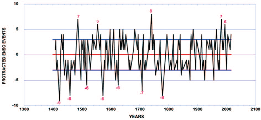
Temporal distribution of ‘protracted’ ENSO episodes in the normalised Niño 4 SST tree-ring reconstruction from the best replicated period from 1400, with instrumental values added on after 1980. The duration in years of extreme ‘protracted’ El Niño (La Niña) episodes are shown by negative (positive) values, with ‘protracted’ episodes equal to, or exceeding ±6 years labelled in red. Horizontal blue lines indicate the −3 (+3) year ‘threshold that designates ‘protracted’ El Niño (La Niña) episodes, respectively.

From the best replicated 1400–2016 period in Figure 4, using normalised values, there are 617 years in total. There are 80 El Niños (13% of the years), of which 35 (5.7%) are ‘classical’ events of 2 years in a row, while exceeding the minimum 3-year criterion, there are 19 ‘protracted’ El Niño episodes of 3 in a row, 15 of 4 (including one of 2013–2016), 7 of 5, 2 of 6, 1 of 7 and 1 of 8. In total, 45 ‘protracted’ El Niño episodes (7.3% of the years). There are 83 La Niñas (13.5% of years), of which 38 (6.2% of the years) are ‘classical’ La Niña events of 2 years in a row, while there are 27 ‘protracted’ La Niña episodes exceeding the minimum 3-year criterion, 4 of 4, 6 of 5, 2 of 6, 2 of 7, 3 of 8 and 1 of 9. In total, there are 45 ‘protracted’ La Niña episodes (7.3% of the years). Combined, there are 163 ENSOs (26.4% of the reconstruction). We would consider in particular that the frequency of the longest of these episodes, such as those labelled on the plot of ±6 years or more, is clearly protracted in nature and appears to exceed in length those in the instrumental record.

This new breakdown indicates that ‘protracted’ El Niño (La Niña) episodes effectively conform to a simple model of ‘classical’ ENSO (fairly equal chance of El Niño or La Niña conditions) events. Interestingly, it also shows the slightly higher tendency for longer La Niña episodes as mentioned in Gergis and Fowler (2009).

Overall, these statistics are consistent with the dynamical perspective discussed in section ‘Overview of the dynamical causes of “Protracted” ENSO episodes’, where the suggested physical processes underlying ‘classical’ events also underlie ‘protracted’ episodes, but operate at different frequencies. They are just different elements/flavours of ENSO, with ‘protracted’ episodes resulting from the interaction between the quasi-biennial, ‘classical’ and quasi-decadal frequency ENSO bands.

The ‘protracted’ episodes seen in the patterns in Figure 3 show the physical structure of these episodes from the recent instrumental record, particularly their tendency for the SST anomalies to extend even further to the west of the Niño 4 region. Additional analysis of relevant palaeoclimatic proxies, such as from both corals and tree rings in the New Guinea–Indonesian region (see potentials in Figure 1 of Freund et al., 2017), could provide evidence as to whether this westward extension of SST anomalies is common in pre-instrumental records.

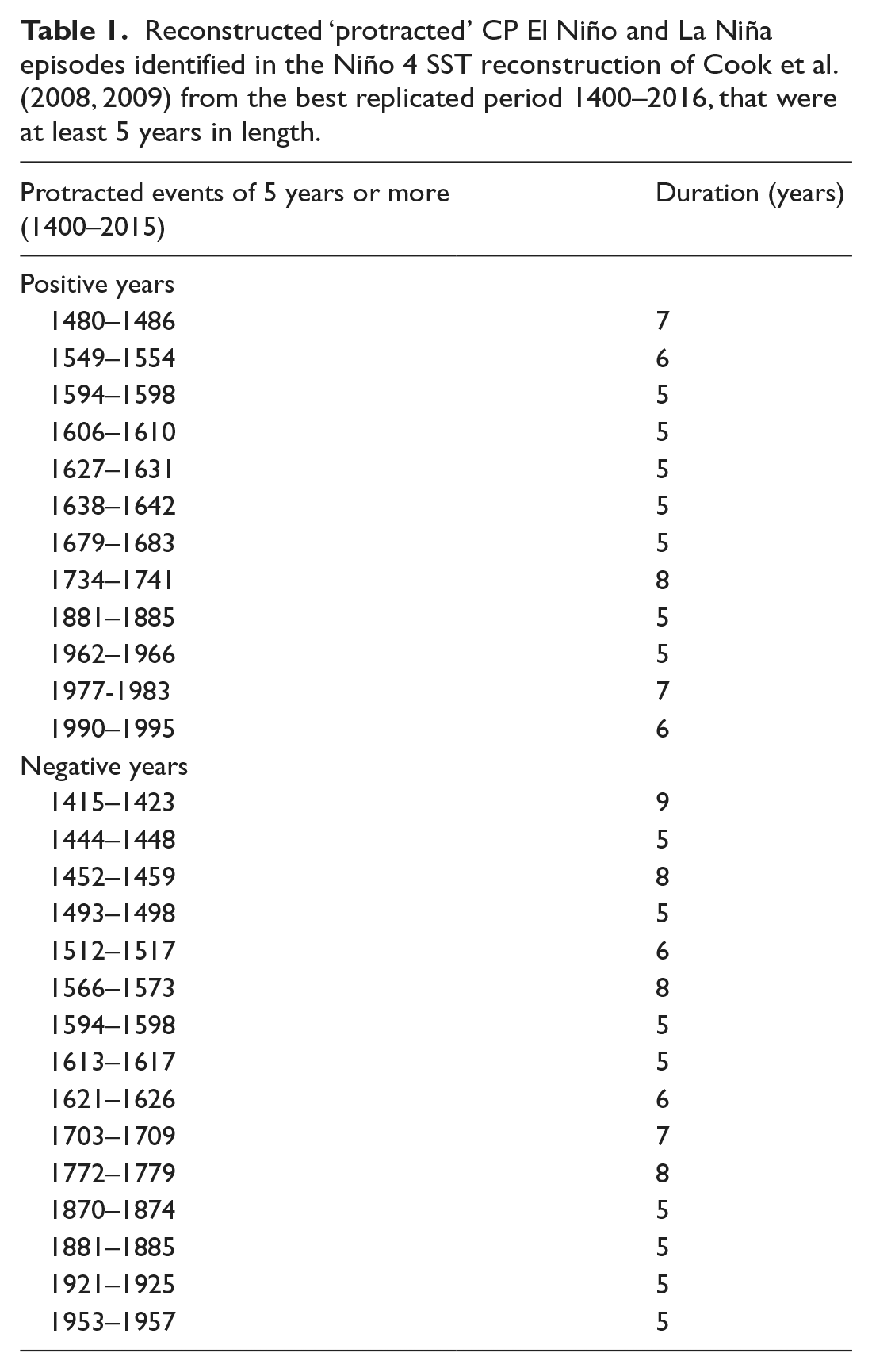
The most recent 2014–2016 Niño is not very unusual in terms of its duration when compared with the longer palaeoclimate record of ‘protracted’ episodes in Table 1. In fact, it only just exceeds the criteria for such episodes, yet its impacts (as described in section ‘Insights into the 2014–2016 protracted El Niño’) were considerable. This also appears to be the case when considering the magnitude of such episodes, while the 2016 DJF instrumental value of 2.37 is the highest in the instrumental record, this value is exceeded in the reconstruction: normalised maximum and minimum values in the instrumental series are 2.37 (2016) and −2.25 (1974), compared with maximum and minimum reconstructed values of 3.34 (1484) and −2.63 (1925), respectively. It thus appears from this analysis that the range of events in the past may have been both more extreme and more protracted than those seen in the recent instrumental period.

OPEN IN VIEWER

Table 1.

Reconstructed ‘protracted’ CP El Niño and La Niña episodes identified in the Niño 4 SST reconstruction of Cook et al. (2008, 2009) from the best replicated period 1400–2016, that were at least 5 years in length.

Protracted events of 5 years or more (1400–2015)	Duration (years)
Positive years
1480–1486	7
1549–1554	6
1594–1598	5
1606–1610	5
1627–1631	5
1638–1642	5
1679–1683	5
1734–1741	8
1881–1885	5
1962–1966	5
1977-1983	7
1990–1995	6
Negative years
1415–1423	9
1444–1448	5
1452–1459	8
1493–1498	5
1512–1517	6
1566–1573	8
1594–1598	5
1613–1617	5
1621–1626	6
1703–1709	7
1772–1779	8
1870–1874	5
1881–1885	5
1921–1925	5
1953–1957	5

Despite these considerations, given the major environmental and societal impacts described in section ‘The 2014–2016 ‘protracted’ El Niño episode and its implications for Australia’, the future risk of extreme ENSO episodes warrants further investigation.

Insights into the 2014–2016 protracted El Niño

A number of papers have examined various aspects of the nature, characteristics and dynamical processes thought to underlie the 2014–2016 El Niño. Some, such as Menkes et al. (2014), Min et al. (2015), Hartmann (2015) and Maeda et al. (2016), have focused on various potential causes of its development in 2014, others such as Lian et al. (2017), Santoso et al. (2017), Hu and Fedorov (2017) and Su et al. (2018) have focused on its strong 2015–2016 signature, while Zhu et al. (2016), L’Heureux et al. (2017), Ineson et al. (2018) and Santoso et al. (2019) examined how well it was predicted. Peng et al. (2018) examined this El Niño in terms of its influence on the Pacific and North American boreal winter of 2014–2015 and suggested that it was indicative of the operation of the North Pacific Mode (NPM) rather than ENSO. However, their NPM SST mode, resolved via a standard EOF analysis of 66 boreal winters in the Pacific domain, showed an SST pattern of close spatial similarity to that of the peak QDO ENSO SST phase in Figure 3. Use of an MTM-SVD or similar approach on seasonal SSTs, where phase structures can be resolved, may have yielded further insight into the dynamical modes involved. Yet, none of these studies have remarked, examined or referred to the protracted nature of this episode.

In this section, we bring together evidence showing the specific nature and characteristics of the 2014–2016 ‘protracted’ El Niño episode. In particular, we contrast and compare the Niño 3.4 and Niño 4 SST regions, indicative of EP and CP ENSO signals, respectively, in terms of their correlation with global precipitation on a seasonal basis, in order to explore the nature of their canonical global patterns and impacts (Figure 5a and b). This is then juxtaposed with the global pattern of drought impacts deduced from the PDSI for the years 2014, 2015 and 2016, which encompassed the latest ‘protracted’ El Niño episode (Figure 6). Finally, sections ‘The 2014–2016 ‘protracted’ El Niño episode and its implications for Australia’ and ‘The Australian responses in sea level’ examine the episode in more detail using the SOI and SST anomalies, and Australian sea level responses.

OPEN IN VIEWER

Figure 5.

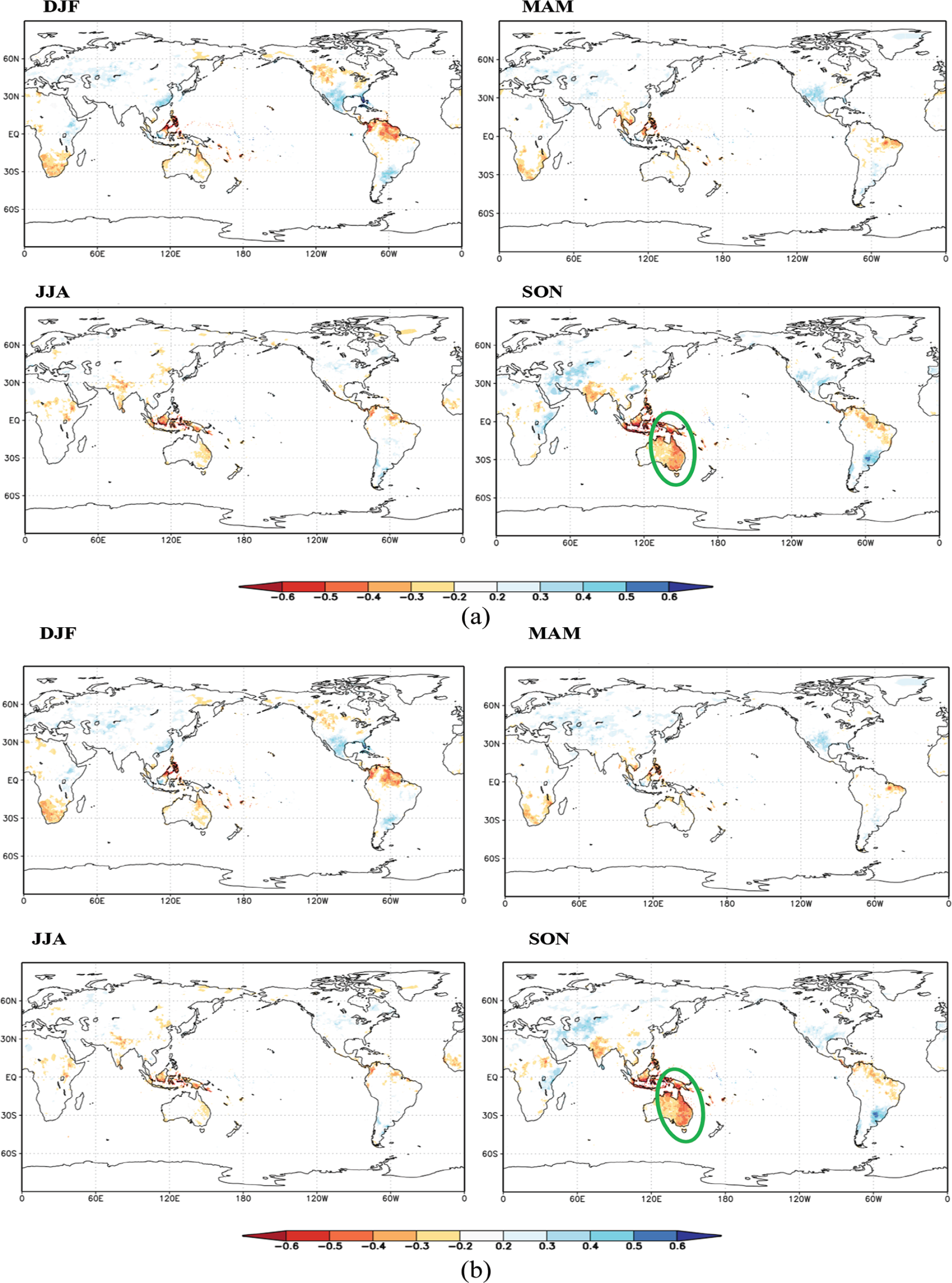
(a) Global and regional seasonal rainfall impacts linked to ENSO events as shown by Niño 3.4 SST–rainfall correlations from 1891 to 2016 (p < 5%). Niño 3.4 SSTs are from ERSSTv5, and rainfall from GPCC V2018 analysis (0.25° resolution): December–January–February (DJF), March–April–May (MAM), June–July–August (JJA) and September–October–November (SON). Correlation values are shown in the bar below the panels. The eastern Australian region is highlighted by the green lozenge. (b) Global and regional seasonal rainfall impacts linked to ‘protracted’ ENSO episodes as shown by Niño 4 SST–rainfall correlations from 1891 to 2016 (p < 5%). Niño 4 SSTs are from ERSSTv5, and rainfall from GPCC V2018 analysis (0.25° resolution): December–January–February (DJF), March–April–May (MAM), June–July–August (JJA) and September–October–November (SON). Correlation values are shown in the bar below the panels. The eastern Australian region is highlighted by the green lozenge.

OPEN IN VIEWER

Figure 6.

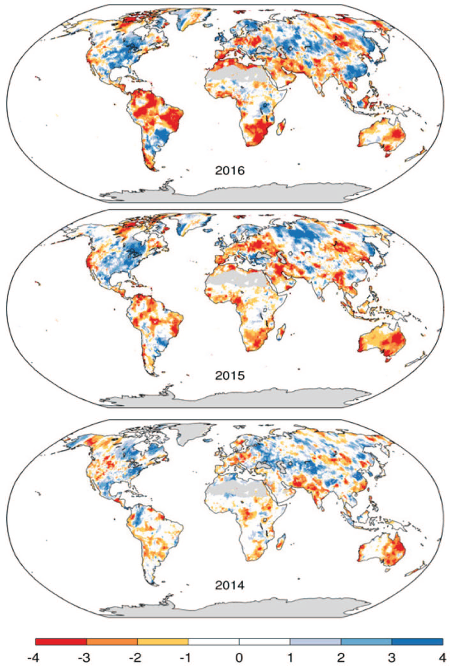
Global drought impacts deduced from the Palmer Drought Severity Index (PDSI) for 2014, 2015 and 2016. Dry (negative) and wet (positive) conditions as shown by the self-calibrating PDSI scale and the colour bar at the bottom of this panel (Osborn, personal communication; https://crudata.uea.ac.uk/cru/data/drought/).

As can be seen in the top block of panels in Figure 5a and b, the global patterns of seasonal Niño 3.4 and Niño 4 SST–rainfall correlations in the 1891–2016 period, indicative of ENSO events and ‘protracted’ ENSO episodes, respectively, have considerable similarity in terms of their regions of most significant impact. However, in eastern Australia, especially in SON (as highlighted in Figure 5b), the Niño 4 SST–rainfall correlations are not only enhanced but more spatially coherent (Murphy and Ribbe, 2004). This then represents a major modulation of wet and dry conditions across this region.

Given the results above, it is not surprising that each of the years of 2014, 2015 and 2016 is characterised by significant drought conditions across the eastern half of the Australian continent, and that this is the most coherent and consistent rainfall impact globally during the 2014–2016 ‘protracted’ El Niño episode. A detailed investigation of this impact is provided below.

The 2014–2016 ‘protracted’ El Niño episode and its implications for Australia

As seen in Figure 7, ‘protracted’ ENSO episodes tend to be dynamically located in the western Pacific. To further investigate the dynamical signatures and impacts of the most recent ‘protracted’ ENSO episode, we now consider the development of this episode and its impacts on eastern Australia.

OPEN IN VIEWER

Figure 7.

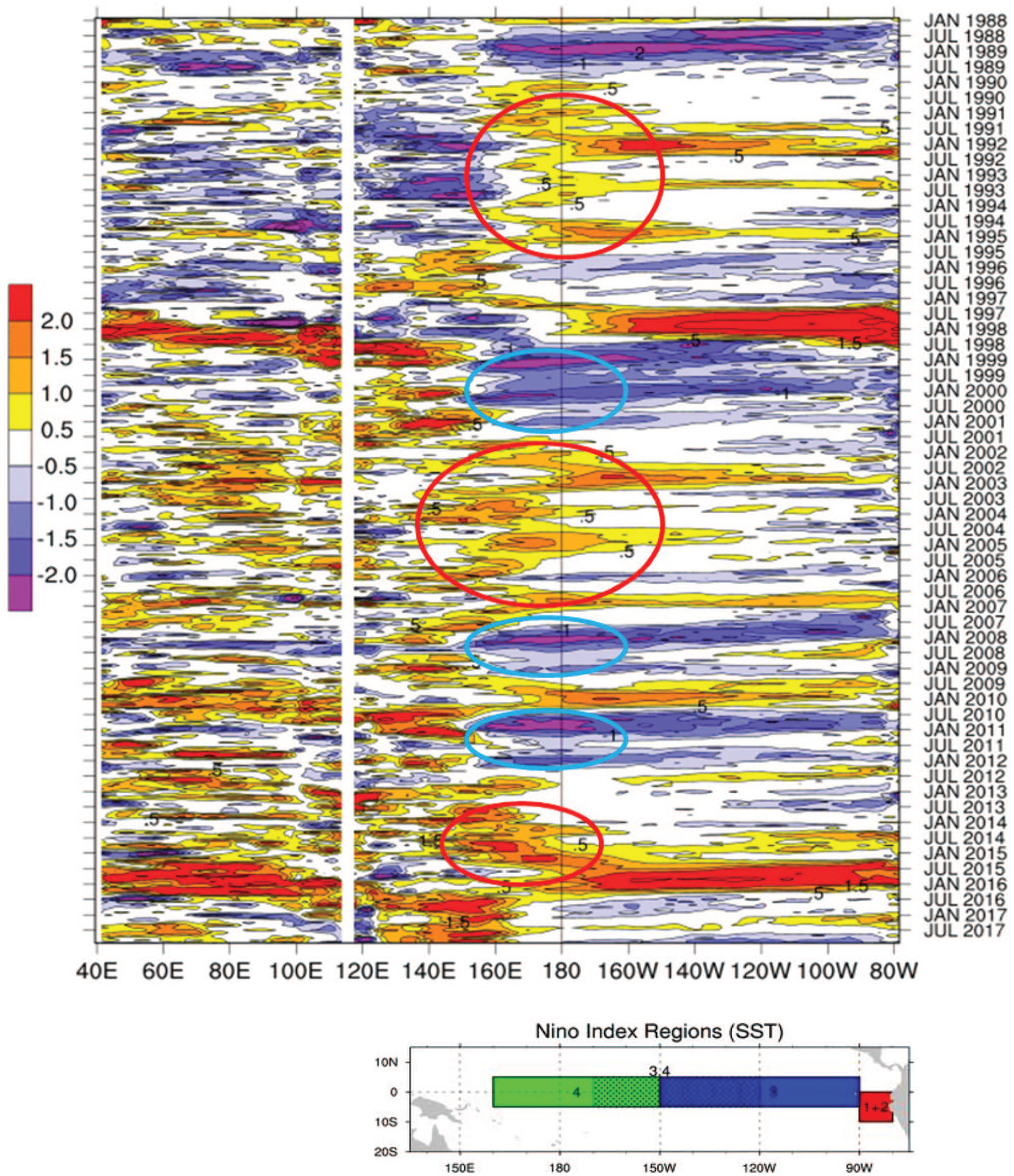
Hovmöller diagram of Indo-Pacific normalised SST anomalies (relative to the 1981–2010 base period) in the tropics averaged from 3.5°N to 3.5°S from January 1988 to July 2017. Red (blue) ovals indicate ‘protracted’ El Niño (La Niña) episodes, and the longitudinal extent of the Niño 4 SST region is shown in the insert at the base of the diagram below the marked longitudes.

During the years of 2014–2016, a prolonged, strong El Niño episode occurred across the equatorial Pacific (Newman et al., 2018; Santoso et al., 2017), as seen in Figure 8. Early 2014 saw raised SSTs indicative of a shift towards El Niño conditions in the Niño 1+2 and 4 regions, when monthly SSTs in the far eastern and western tropical Pacific respectively increased between March and June 2014, with warming in the Niño 4 region by up to 0.77°C above average (OISST.v2, 1981–2010 base period) (Figure 8). In contrast, strongly positive SSTs in the Niño 3 and/or 3.4 regions, used in operational definitions and monitoring of El Niño conditions by most international climate agencies, only clearly registered warming later in November 2014. MSLP observations from NOAA’s Climate Prediction Center (http://www.cpc.ncep.noaa.gov/data/indices/) indicate that the atmosphere failed to couple with the ocean until around August 2014 (Dong and McPhaden, 2018).

OPEN IN VIEWER

Figure 8.

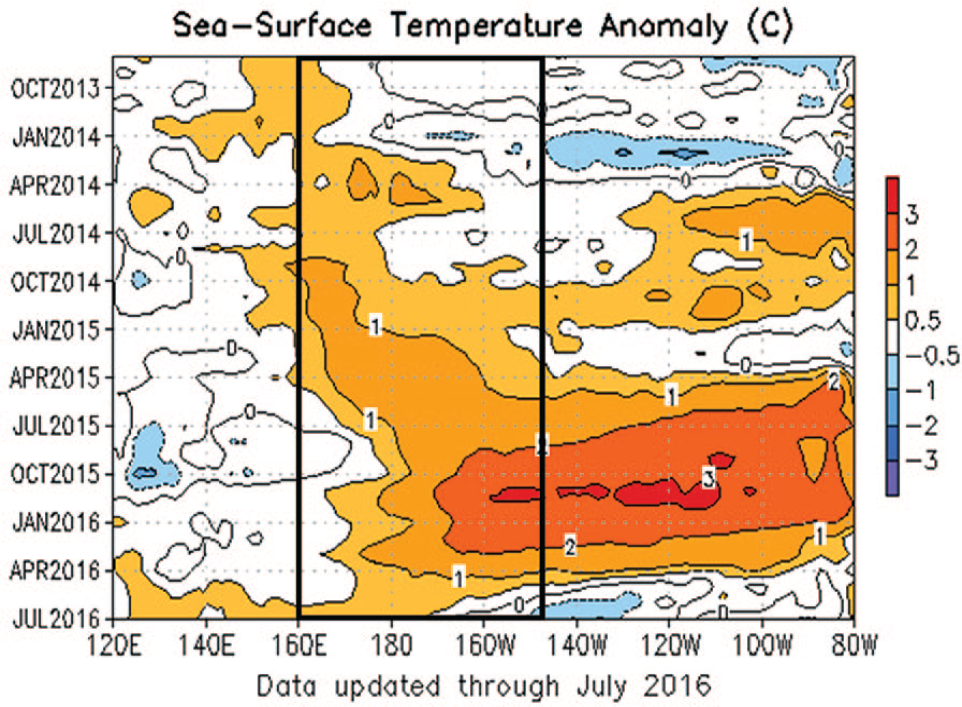
Time–longitude section of monthly anomalous sea surface temperature (SST) averaged between 5 N and 5 S. Contour interval is 0.5 C. Dashed contours indicate negative anomalies. Anomalies are departures from the 1981–2010 base period means (Smith and Reynolds, 1998). The Niño 4 region is shown by the black rectangle.

Although positive MSLP values were recorded over Darwin from as early as March 2014, the SOI did not reach El Niño levels in the EP until August 2014. From February 2015, Niño 4 SSTs remained more than 1°C above average until March 2016. This strong warming was reflected in Niño 3.4 SSTs from May 2015 to April 2016, peaking at a record high of 2.95°C above average (1981–2010 base period) in November 2015. This followed highly negative SOI values from May to October 2015, with particularly high MSLP anomalies recorded at Darwin in October. Ocean temperatures in the Niño 4 and Niño 3.4 regions remained anomalously high until April 2016 (also associated with the peak value of the SOI recording during this event), when El Niño conditions finally began decaying during the austral winter. The evolution of the 2014–2016 ‘protracted’ El Niño episode is mentioned in the Bulletin of the American Meteorological Society State of the Climate reports from 2015 to 2017 in Blunden and Arndt (2015, 2016, 2017), Parker et al. (2016) and Oliver et al. (2017). Similarly, the 2010–2012 ‘protracted’ La Niña episode is detailed in Blunden and Arndt (2012, 2013, 2014).

The ‘protracted’ 2014–2016 El Niño resulted in major environmental and societal impacts across the globe. In the western Pacific, severe drought and associated food shortages impacted Papua New Guinea, Indonesia and many Pacific islands nations including Vanuatu, Fiji and the Solomon Islands (Cook et al., 2016). During 2015, Singapore was badly affected by enhanced air pollution due to wildfires in Indonesia linked to major drought conditions (Lee et al., 2017). Rainfall deficits over Australia from September to November 2015 resulted in Australia’s third driest spring on record, the season when Australian rainfall is most influenced by ENSO variability (Risbey et al., 2009). This resulted in reduced crop production in the country’s largest agricultural region of the Murray–Darling Basin (Cook et al., 2016). A combination of high temperatures and low rainfall brought a very early start to the Australian bushfire season, with more than 130 fires burning in Victoria and Tasmania in October 2015 at the peak of the El Niño. By January 2016, abnormally dry conditions in the temperate region of Tasmania saw hundreds of fires started by dry lightning, damaging large areas of the Tasmanian Wilderness World Heritage Area, including rainforest and peatlands that have not experienced fire for centuries (Bowman, 2016; Cook et al., 2016).

In north-eastern Australia, persistently high SSTs and fewer clouds due to a weakened monsoon contributed to unprecedented coral bleaching of the Great Barrier Reef, which spans 2300 km along the eastern Australian coast (Hughes et al., 2017; Hughes and Kerry, 2017). Following record high SSTs in 2016, the north-eastern Australia region experienced its first occurrence of back-to-back mass bleaching across two-thirds of the world’s largest reef system during 2015–2016 and 2016–2017, resulting in the mortality of 50% of the coral in the reef ecosystem (Hughes et al., 2017; Hughes and Kerry, 2017). While under the influence of a major southward extension of the East Australian Current, both during and following the 2014–2016 ‘protracted’ El Niño episode, these anomalously warmer SSTs displaced tropical and sub-tropical marine species and caused ecological impacts as far as the Tasman Sea region (Brown, 2014; Oliver et al., 2017). In contrast, McGowan and Theobald (2017) have suggested that above-average atmospheric pressure experienced during El Niño events results in reduced cloud cover and increased air temperatures that play a more crucial role than large-scale SST warming alone in determining the extent and location of coral bleaching of the Great Barrier Reef.

While research into the causes of mass coral bleaching associated with this ENSO episode is still underway, it is clear that substantial threats of future bleaching exist during periods of prolonged warming. Aside from the intrinsic value of being an area of exceptional biodiversity, a recent analysis has estimated that the Great Barrier Reef generates over 64,000 jobs and contributed $6.4 billion to the Australian economy in 2015–2016 (Deloitte Access Economics, 2017). The significant impact of these prolonged El Niño conditions has raised serious concerns about the future risk of ENSO extremes in the region, prompting this analysis into past ENSO behaviour and its possible dynamical causes.

The Australian responses in sea level

Although the Australian rainfall response to ‘protracted’ episodes is centred on eastern parts of the continent, we have also looked at the bigger picture with Australia-wide sea level observations. In Supplementary Figure S4 (available online), the SST response in tropical Australian waters occurs to the northwest, north and northeast of Australia in correlations with Fremantle, Darwin and Townsville sea anomalies, which peak during the austral spring.

Allan et al. (1990) showed that anomalies in seasonal sea level from northern Australian tide gauges at Darwin and Port Hedland correlated more strongly, spatially and both simultaneously and at lags with seasonal Australian district rainfall fluctuations than the more familiar correlations with the SOI, northern Australian SSTs or Darwin MSLP. This enhanced response is primarily due to the integrating effect of meteorological influences, primarily the inverse barometric effect, SSTs and winds, on sea levels.

As shown in Figure 9, this response can be tracked in sea level, extending from northern Australia anti-clockwise around the Australian continent to its north-eastern coast. Unfortunately, at the time of Allan et al.’s (1990) paper, any enhancement of statistical seasonal forecasting approaches through the use of this sea level response was thwarted by the then slow data transmission responses from those Australian tide gauges and their flow into seasonal forecasting approaches in any real-time sense. This has now been overcome by major improvements in technology and data streaming from the array of telemetering tide gauges around Australia and internationally. However, although satellite altimetry data are assimilated into seasonal sea level forecasts using dynamical models, tide gauge observations are not.

OPEN IN VIEWER

Figure 9.

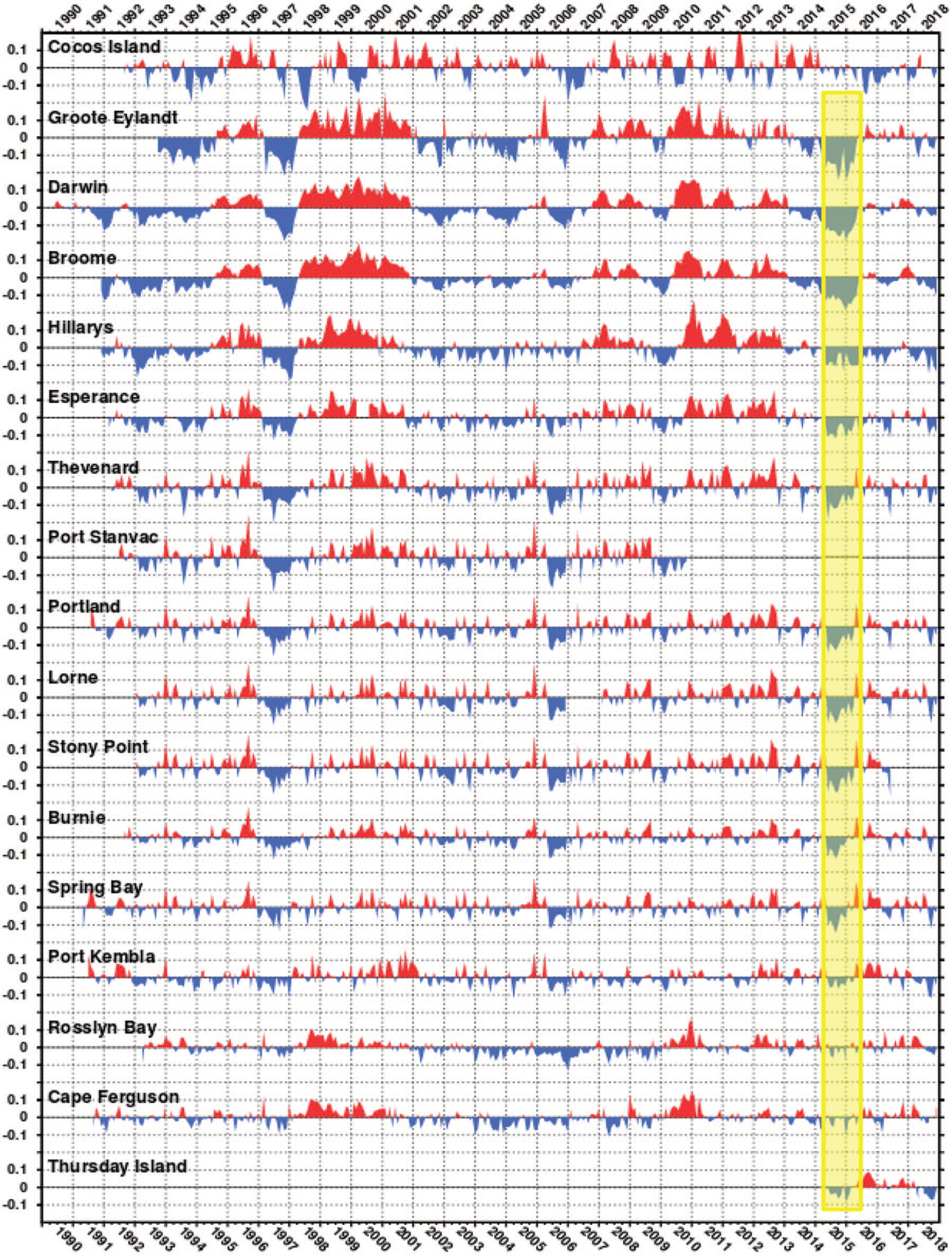
Monthly sea level anomalies from 1990 to December 2018 counter clockwise around Australian coast. The transparent yellow shaded region shows the extent of the 2014–2016 ‘protracted’ El Niño episode.

As seen in Figure 9, significant Australian sea level responses are not only restricted to seasonal fluctuations, generated by phenomena such as ENSO, but also respond on quasi-decadal timescales and thus to ‘protracted’ ENSO episodes. This is most strongly evident with the negative sea level anomalies around the entire Australian coast during the 2014–2016 episode, and also, though mainly in the more tropical coastal regions, during the 1990–1995 and 2002–2005 ‘protracted’ El Niño plus 1999–2001 and 2010–2012 La Niña episodes. This is even seen to extend out into the Indian Ocean, with even more coherent sea level anomaly responses to both ‘classical’ ENSO events and ‘protracted’ ENSO episodes in the Cocos Island tide gauge record and is in line with the broader spatial pattern of altimetry/sea level seen in Figure 2c. As Lyu et al. (2017) indicate,

Our results suggest that the observed sea level variations as well as the derived short-term trends should be interpreted in the context of sea level variability on multiple time scales, which are linked to different climate processes and thus show distinct spatial patterns.

A comparison of the wavelet characteristics of the SOI (1866–2019), Niño 3.4 SST (1854–2019), Niño 4 SST (1854–2019) instrumental series with Australian sea level anomalies at Darwin (1959–2016) and Fremantle (1897–2018) (see Supplementary Figure S3, available online) shows that the more tropical instrumental series based on MSLP and SST display strongest power centred on ‘classical’ ENSO frequencies. However, Australian tropical (Darwin) and mid-latitude (Fremantle) sea level series are dominated by more quasi-decadal signals. With reference back to the panels in Figure 2c, showing SOI and altimetry (satellite-derived sea level) correlations plus quasi-decadal steric height fields in the first EOF of sea level variations in the Pacific and around Australia, these results further establish seasonal sea level anomalies as an additional measure of both ‘classical’ and ‘protracted’ ENSO episodes across the Indo-Pacific region.

However, with other parameters, such as OHC and SSS, the pattern is different, in that the response is only in waters to the north and west-northwest of the continent (seen particularly in SON sea level anomaly correlations with SST, OHC and SSS anomalies in Figure S4, available online in the Supplementary Material). When examined in conjuncture with online maps of seasonal 925 and 200 hPa velocity potential anomalies during the 2014–2016 period (not shown), strong overturning of mass was seen between the eastern Australian (strong subsidence) and Niño 4 SST regions (strong upward vertical motion). The period is dominated by low-level (925 hPa) flow directed away from eastern Australia (particularly over Queensland) with upper level (200 hPa) counter/return flow coming into eastern Australia aloft. This enhanced subsidence, which suppressed rainfall and enhanced drought conditions across eastern Australia. The OHC and SSS response would most likely have other effects on the marine ecosystem in northern and western seas of Australia.

Conclusion

As seen in section ‘The 2014–2016 ‘protracted’ El Niño episode and its implications for Australia’, longer ‘protracted’ ENSO episodes have the potential to exacerbate societal, agricultural, environmental and ecological impacts experienced during shorter ‘classical’ (and usually stronger) ENSO events documented elsewhere (e.g. Power et al., 1999). This is manifest by major fluctuations in Indo-Pacific to global atmospheric, oceanic, terrestrial and marine environments, especially through fluctuations in MSLP, SST, sea level and also OHC and SSS. In fact, a similar mechanism put forward to explain the ocean–atmosphere dynamics for ‘classical’ ENSO events has also been suggested to operate with ‘protracted’ ENSO episodes, when the QDO ENSO signal dominates. Thus, it should be a target for the international decadal forecasting community (Power et al., 2017).

Although globally impacting similar regions affected by ‘classical’ ENSO events, ‘protracted’ ENSO episodes last longer and are most pronounced in the eastern Australian sector. This can be seen in Australian sea level anomalies from coastal tide gauges since 1990 and is most coherent and extensively recorded right around the Australian region during the ‘protracted’ 2014–2016 El Niño episode.

Our preliminary examination of palaeoclimatic records of ENSO indicates strongly that ‘protracted’ ENSO-type events have occurred prior to the instrumental record. The long Niño 4 SST reconstruction demonstrates that the most recent ‘protracted’ 2014–2016 episode was not particularly distinctive with regard to either its length or severity relative to those that have occurred in the past. What is seen from palaeoclimate reconstructions is that the range of past ‘protracted’ ENSO episodes in this reconstruction, which peaked in the 14th to 18th centuries, with many lasting 6 or more years, has not been observed in modern instrumental records. This suggests that shorter instrumental observations may underestimate the risks of possible future ENSO extremes compared with those observed from multi-century palaeoclimate records. While instrumental records provide a much finer temporal resolution of ‘protracted’ ENSO episodes, unfortunately, they are limited in length, so ideally should be supplemented with high-quality, high-resolution, long-term palaeoclimate records wherever possible to examine low-frequency variations in ENSO behaviour. Improved knowledge of ENSO and the potential to forecast protracted episodes would be of immense practical benefit to communities particularly in western Pacific regions like eastern Australia where the impacts of ENSO extremes are especially severe.

Supplemental Material