A ~1000-year 13 C Suess correction model for the study of past ecosystems

Abstract

Inferences about how an ecosystem has changed through time often rely on longitudinal records of species characteristics or niche parameters, and stable isotope analysis is a common tool employed to study changes in an organism’s niche. One of the most frequently used stable isotope measures is δ¹³C, a ratio of ¹³C to ¹²C. However, applying δ¹³C to historical samples comes with some methodological hurdles. One such hurdle is correcting for the ¹³C Suess effect or the change in atmospheric δ¹³C due to increased anthropogenic CO₂ emissions. The change in the amount of carbon isotopes in the atmosphere through time can confound the study of historical shifts in species characteristics. No standard way of correcting for the ¹³C Suess effect has been suggested despite this problem. Here, I propose a standard ¹³C Suess correction model for the past ~1000 years using three prehistoric/historic records of atmospheric δ¹³C.

Keywords

anthropogenic carbon emissions carbon isotopes historical ecology paleoenvironments stable isotopes

Introduction

Stable isotope analysis has helped clarify baseline information regarding the niche (sensu Newsome et al., 2007b) of past organisms and how niches change or remain constant through time. Historical shifts in animal diet, habitat preference, migration, and reproduction have been tracked using stable isotopes (Braje et al., 2017; Chamberlain et al., 2005; Fox-Dobbs et al., 2007; Hofman et al., 2016; Koch et al., 2017; Newsome et al., 2007a, 2007b, 2010; Reid et al., 2018). However, employing this technique comes with some methodological hurdles.

One hurdle concerns the ¹³C Suess effect (Keeling, 1979; Keeling et al., 1979), which greatly impacts the biological carbon cycle. The biological carbon cycle is the term used to describe how atmospheric carbon enters and travels through food webs (see Sharp, 2017, Chapter 7 for a detailed overview). The ¹³C Suess effect is the change in the ratio of ¹³CO₂ to ¹²CO₂ in the atmosphere due to increased anthropogenic fossil fuel emissions. Burning coal/lignite, petroleum, and natural gases and producing cement force an acceleration of the biological carbon cycle by rapidly releasing large amounts of carbon that took millions of years to store in Earth’s sediments (Yakir 2004: 181). Most of the carbon released from anthropogenic fossil fuel emissions is the lightest carbon isotope, ¹²C. Two major photosynthetic pathways fix ¹²CO₂ or ¹³CO₂ differently. The C₃ photosynthetic pathway fixes more ¹²CO₂ than ¹³CO₂ compared with the C₄ photosynthetic pathway. The average δ¹³C value of C₃ plants is around −28‰ while the average value is around −13‰ for C₄ plants (Fry, 2007:63). Over the Earth’s history, the majority of biomass converted into fossil hydrocarbons used the C₃ photosynthetic pathway (e.g. phytoplankton (Schidlowski and Aharon, 1992) or just general plant biomass from the Cretaceous (Berner, 2003)). The evolution of the C₄ photosynthetic pathway is a geologically recent event perhaps first occurring some 24–35 million years ago during the Oligocene epoch (Cerling et al., 1998; Ehleringer et al., 1997; Sage, 2004). Therefore, the concentration of ¹²CO₂ has increased in the atmosphere with the onset of increased fossil fuel emissions starting with the Industrial Revolution (ca. AD 1760). To reiterate, human activity has pulled ¹²C out of long-term storage in fossil fuels and has put it back into the atmosphere. More ¹²CO₂ in the atmosphere translates to an increase in the amount of ¹²C in the global carbon cycle.

This change in the amount of ¹²C relative to ¹³C in the atmosphere presents a methodological problem: if a researcher has measured δ¹³C in tissues of both past and present organisms, then the ratio of ¹³C to ¹²C in the atmosphere is likely different between the two times. The ratio increases from the present into the past. Observed changes in the carbon isotope composition of animal or plant tissue through time could be attributed to the changing amount of different carbon isotopes in the carbon cycle rather than the phenomena that the analyst set out to measure. In short, there is a baseline shift in the concentration of different carbon isotopes in the atmosphere through time that can cause a problem of equifinality.

There is no standard way that historical stable isotope ecologists account for the ¹³C Suess effect. One reason for the lack of standardization is that a sufficient correction is largely dependent on the kinds of questions or the kind of dataset that the analyst has. For instance, the contemporary stable carbon isotopic composition of the atmosphere is frequently measured and the pre-1760 composition is widely agreed upon. If an analyst has a contemporary sample that they want to compare with a pre-1760 sample, then the correction is straightforward: take the difference in the stable carbon isotope composition of pre-1760 atmosphere (δ¹³C = approx. −6.4‰) and the contemporary atmosphere (δ¹³C = approx. −8.4‰). The researcher can either subtract the difference from the pre-1760 sample or add it to the contemporary sample. However, if the more recent sample of interest spans anywhere between 1760 and the present day, then the correction value that should be applied becomes ambiguous. However, this ambiguity has been handled in different ways (see for instance Chamberlain et al., 2005; Long et al., 2005; Reid et al., 2018; Schelske and Hodel, 1995).

Normally, ¹³C Suess corrections are estimated as a means to an end: solving environmental or social problems. Thus, it is no surprise that a standard ¹³C Suess correction curve has not been established. Such a curve, however, would be useful so that researchers would not need to develop new ones for the problems they are trying to solve. Here, I propose an easy-to-use model that provides a standardized way to produce year-by-year ¹³C Suess effect correction values. This model predicts the ratio of ¹³C to ¹²C in the atmosphere by using well-established empirical records of δ¹³C from Antarctic ice cores, firn air, and flask samples (Bauska et al., 2015; Rubino et al., 2013; White et al., 2015).

Methods

I combined three different datasets to produce the model presented here. The datasets were of carbon isotope values measured in atmospheric carbon dioxide trapped in various physical media. The first dataset comes from the West Antarctic Ice Sheet Divide ice core (Bauska et al., 2015) and includes 69 carbon isotope values between AD 753 and 1916. The second dataset combines ice core and Firn air samples collected at Law Dome and South Pole, Antarctica (Rubino et al., 2013). This dataset reports 156 carbon isotope values between AD 1019 and 2001. The third dataset comes from the National Oceanic and Atmospheric Administration and consists of monthly air samples collected in glass flasks from the South Pole, Antarctica, from 2002 to 2014 (White et al., 2015). I report carbon isotope values in delta (δ) notation using the following calculation: ((R_sample/R_standard − 1) × 1000), where R_sample is the ratio of ¹³C to ¹²C of air trapped in ice, collected by a Firn Air Sampling Device or in a glass flask. R_standard is the ratio of ¹³C to ¹²C in Vienna Pee Dee Belemnite, which is an internationally accepted standard. There is a slight offset between the two ice core records from Law Dome and West Antarctic Ice Sheet Divide (~0.08‰), which is attributed to the use of different reference schemes (Bauska et al. 2015: 383). This offset is low and has little to no impact on the accuracy of the model presented.

I used locally estimated scatterplot smoothing (LOESS) to fit a curve to these combined datasets in R (v 3.5.1; see Supplementary File 1, available online). LOESS is a non-parametric regression method that fits multiple regression models together one subset (or span) of a scatterplot at a time (Cleveland, 1979; Cleveland et al., 2017). One of the greatest advantages of using LOESS is that it does not require an a priori assumption about the shape of the data it is applied to, unlike linear regression or polynomial regression. Thus, this method is appropriate to apply to a dataset concerning historical fluctuations of δ¹³C in the atmosphere because a theoretical model that could explain such fluctuations would be incredibly unwieldy. Tracking the exact carbon isotope ratio of the fossil fuels used in different periods of time, the rate of use of different fossil fuels, the effect of incomplete combustion, and so on, is a near impossible task. The LOESS algorithm in R can issue errors if there are repeated values at a relatively high frequency. The mean was taken for all δ¹³C values associated with repeating years, which applies to the datasets from Bauska et al. (2015) and Rubino et al. (2013), to avoid this problem. In addition, the mean of monthly δ¹³C values was used for each year between 2002 and 2014, which applies to the dataset from White et al. (2015). The lowest span that resulted in no warnings or errors was used to create a curve with the highest smoothing resolution (span = 0.10 or an approximately 127-year span).

Results

The ¹³C Suess correction model predicts atmospheric δ¹³C for 1266 years (AD 753–2019) with extremely low error (standard error ⩽ 0.1‰). Pre-Industrial Revolution – pre-AD 1760 (Ashton, 1997) – values are relatively stable, hovering around −6.4‰ (Figure 1). Interestingly, there is a small, but rapid, dip in δ¹³C starting around AD 1425/1450 (on the order of 0.1‰). The rebound from this dip occurs at the start of the large-scale depopulation of the Americas due to European arrival, recently termed the Great Dying (AD 1520–1700). Researchers have argued that abandonment of agricultural land – due to the massive population loss of indigenous peoples – caused this uptick in δ¹³C. Abandoned agricultural land would have underwent secondary succession, which in turn would have increased global ¹²C fixation (see Koch et al., 2019). One implication of this argument is that the impact this event had on the carbon cycle might have been the start of the Anthropocene. From an isotopic perspective, the Industrial Revolution (AD 1760–1830) was far more globally impactful. There has been an approximate 2.0‰ decrease in δ¹³C from the Industrial Revolution to the present day.

Figure 1.

The ¹³C Suess correction model developed here that uses ice core, firn air, and flask sample data (Bauska et al., 2015; Rubino et al., 2013; White et al., 2015). The historical time periods known as the Great Dying (AD 1520–1700) and the Industrial Revolution (AD 1760–1830) are highlighted in orange to anchor this model to two historical events that argued to have drastically changed the global carbon cycle. The Great Dying is the large-scale depopulation of the Americas due to European arrival, which is a term recently coined by Koch et al. (2019).

Supplemental File 1, available online, provides the raw data used to create the curve, and Supplemental File 2, available online, is an R Markdown PDF of the code used to create the curve and to export the DataFrame of predicted δ¹³C values of atmospheric carbon for each year. I have also converted that DataFrame into an easy-to-use Excel spreadsheet (XLSX file; Supplemental File 3, available online). An example of how to determine the ¹³C Suess correction value between AD 755 and 2007 is illustrated in Supplemental File 3. The only other step the analyst must take after calculating the correct ¹³C Suess correction value is whether to add it to a modern sample or subtract it from a past sample (see below for more detail on that decision).

Discussion

Important practical concerns emerge, given the ¹³C Suess correction curve presented above. Such concerns relate to the usefulness of a correction that is (at worst) 2.0‰, if this correction curve can be used in different habitat types where the carbon cycle is much different (i.e. marine versus terrestrial), how seasonal shifts in atmospheric δ¹³C relate to this model, and how correction values should be applied to samples. I tackle each of these topics below in hopes of allaying their related concerns.

How much is 2.0‰, really?

Marion H. O’Leary (1988) wrote,

The precision of modern mass spectrometers is at least ±0.02 ‰, but sample preparation errors may bring the total reproducibility of measurements on plant materials to ±0.2 ‰. Thus, interpretations based on differences smaller than 1 ‰ should be made with caution. (p. 328, emphasis added)

This statement has become almost axiomatic in the field of isotope ecology, and it is remarkable that this statement remains relevant even after the technological advances of the last ~30 years. But what about 2.0‰? Is the ¹³C Suess effect really in need of correcting if it is, at worst, different by about 2.0‰ from the present day compared with around 1000 years ago?

Differences of only a couple of per mil can matter when researchers make arguments based on such slight differences. For instance, Grimstead et al. (2016) compared bioapatite stable carbon isotope values from archaeofaunal and contemporary rodent and lagomorph specimens, and they argued that past humans procured small animals from maize-based agricultural plots (Figure 2a). Their record of modern small animals was curated over a 44-year period (from AD 1948 to 1992). However, a constant (1.5‰) ¹³C Suess correction was applied to the data, even though the δ¹³C value of atmospheric carbon was unstable over that time. Applying a year-to-year ¹³C Suess correction to these data highlights potential overlap in the values reported by the authors (Figure 2b): the 1‰ buffer between agricultural and non-agricultural small animals that existed with the original constant Suess correction disappears with a time-sensitive one. Importantly, this exercise does not dramatically alter the conclusions of the authors, but it does highlight nuance that future archeologists should take into account. The question that remains is how different does a bioapatite δ¹³C value have to be to consider a small animal hunted in an agricultural or non-agricultural plot?

Figure 2.

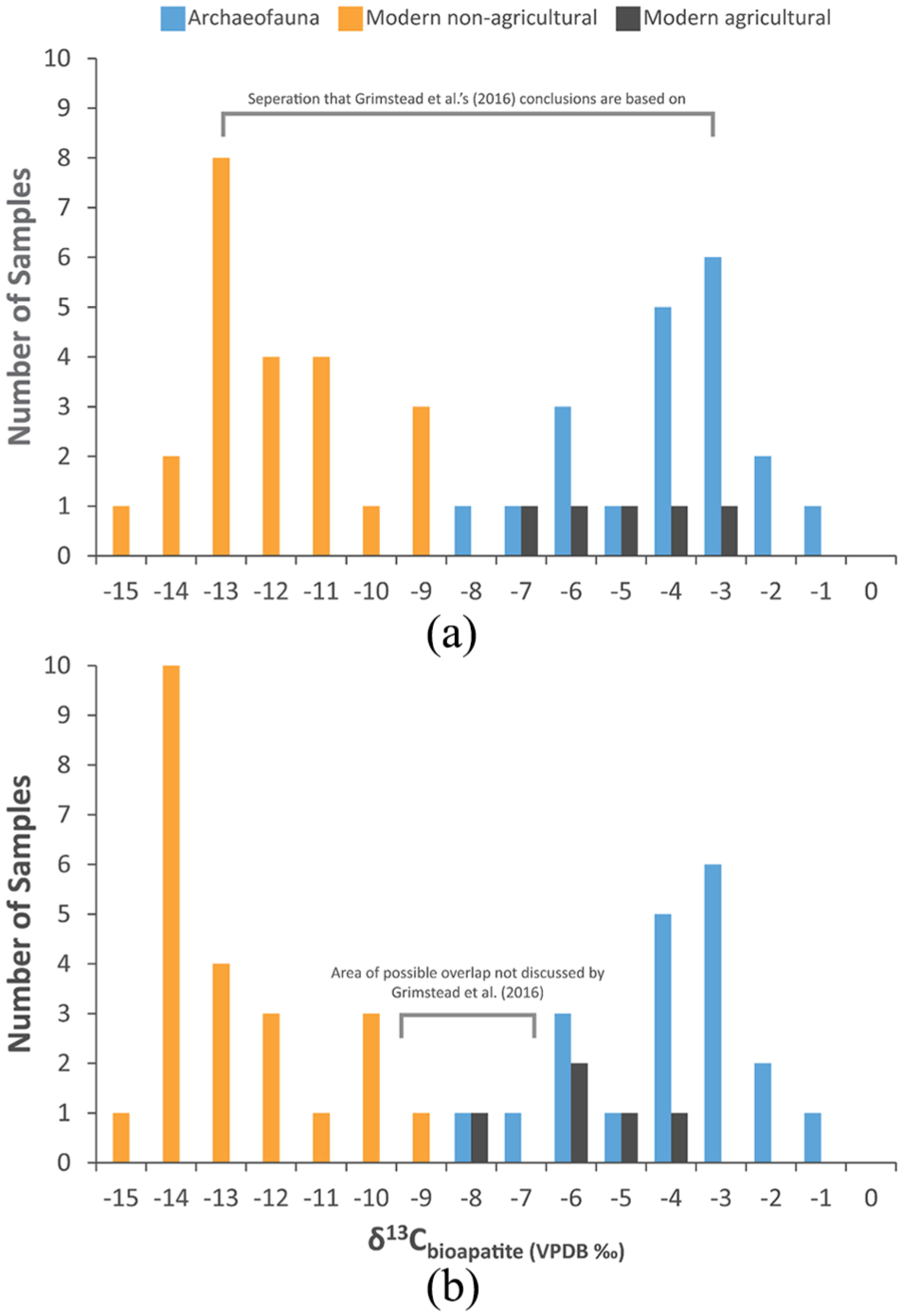
(a) Histogram of bioapatite δ¹³C values from archeological lagomorphs and rodents recovered from the prehistoric American Southwest (i.e. archaeofauna from Chaco Canyon, New Mexico) along with modern lagomorphs and rodents from non-agricultural/agricultural contexts sampled from museum collections (reproduced from Grimstead et al., 2016). The curation of these museum specimens occurred over a 44-year time span (AD 1948–1992) at the Museum of Southwestern Biology in Albuquerque, New Mexico. However, a constant 1.5‰ ¹³C Suess correction was applied to them. (b) The same dataset from Grimstead et al. (2016) but with the year-to-year ¹³C Suess correction values developed here applied. This figure demonstrates how different Suess correction protocols can change inferences made by researchers.

In addition, it is important to remember that small differences in δ¹³C values are associated with important changes in an organism’s niche. Any longitudinal record designed to clarify an organism’s trophic positioning through time that uses δ¹³C is heavily influenced by the type of ¹³C Suess correction used. Differences in carbon isotope values of a consumer and its food (Δ¹³C_{predator−prey}) can be extremely small, sometimes on the order between 0‰ and 2‰ (Bocherens and Drucker, 2003). Suess corrections can also significantly impact historical biogeographic interpretations, like where an animal ate or reproduced through time. Geographic baseline shifts in isotope values can be small. For example, the δ¹³C values of past pinnipeds measured from bone collagen vary only around 1‰ between the Western Aleutians, the Northern Pacific, and the Southern Pacific (see Newsome et al., 2007a).

So, is the ¹³C Suess effect really in need of correcting? Yes. The ¹³C Suess effect is historically measurable to a more than sufficient degree and clearly impacts interpretations based on δ¹³C values. A difference of 2.0‰ in δ¹³C space can have serious ramifications on historical interpretations no matter if those interpretations are about the longevity of past human subsistence practices or about the historical biogeography of a seal species. Researchers who want to compare historical niche shifts are unintentionally propagating error in their datasets if they do not account for the Suess effect. Even a small amount of error spread through a dataset can have significant impacts on inference testing. Given large enough sample sizes, certain inferential tests can make small differences seem like highly significant ones. This is especially the case when one overrelies on p values (see Wolverton et al., 2016).

Terrestrial versus marine

Cores taken from ice sheets record terrestrial processes through the accumulation of precipitation (i.e. snow and ice) on Earth’s crust. Thus, the model presented here applies to the terrestrial carbon cycle. How the ¹³C Suess effect has impacted the marine carbon cycle has been the topic of considerable debate. This debate involves baleen whales (Mysticeti), which may represent a good proxy for primary productivity in the ocean. They consume zooplankton, and zooplankton feed on phytoplankton. Schell (2000) used 37 different bowhead whale (Balaena mysticetus) baleen plates sampled from 1947 to 1976 and two archeologically recovered baleen plates to produce a longitudinal record of primary productivity in the Bering Sea. This longitudinal record showed a decline in δ¹³C through time, which could have been indicative of a drop in the amount of carbon fixation (i.e. less photosynthesis and by extension less primary productivity). Such a drop in primary productivity would have significantly impacted the number of species the sea could support, but this assertion was challenged (Cullen et al., 2001). The longitudinal record produced from baleen plates did not account for how anthropogenic carbon emissions might have dissolved into ocean surface water and how a change in the concentration of CO₂ in ocean water might force an alteration in how phytoplankton fractionate carbon during photosynthesis. What matters here is that the original record was challenged because it did not sufficiently account for the ¹³C Suess effect. The primary assumption issued in this challenge was that the ocean must be in complete global equilibrium with the atmosphere. That assumption was disputed, and another one was put forward: deep water in upwelling regions and high latitude zones is less impacted by anthropogenic CO₂ (Schell, 2001). More recently, the mechanism that drives change in δ¹³C values in such areas has been more thoroughly explained (Williams et al., 2011: 170), and a global estimate of the oceanic ¹³C Suess effect has been put forward (Eide et al., 2017). The model presented here should not be used in marine systems.

Seasonality

There is intra-annual or seasonal variation in atmospheric δ¹³C based on differing rates of fossil fuel emission or the amount of vegetation that is fixing carbon, but such variation can be rather small. For instance, the dataset I used from White et al. (2015) has around nine δ¹³C values taken at different times of the year. The average standard deviation of δ¹³C values within each year from this dataset is 0.02‰. Regardless of the low amount of variation, the atmospheric carbon isotope ratios provided here should be thought of as time-averaged values for each year. The analyst must be prepared to assess how seasonality might influence the stable carbon isotope values they have measured from their species of interest.

Whether backward or forward

A researcher is faced with a very specific question when applying Suess correction values: should I correct my historical data to look contemporary or should I make my contemporary data look historical? Ultimately, the answer should depend on the goal of the study. If the goal is to understand how past environments and organisms operated by comparing past organisms with modern ones, then it would make most sense to add the Suess correction value to the more recent sample. If the goal is to make modern-day recommendations, then it would make sense to subtract the Suess correction from the older sample. Regardless of how one chooses to employ ¹³C Suess correction values presented here, what is most important is that the analyst clearly explains how they went about making corrections and why they made the choices they did. Remember that 2.0‰ can really matter. Not being clear about how that amount is applied to a sample can lead to confusion in the literature.

Conclusion

I created a high-precision ¹³C Suess correction curve for the last 1266 years using pre-existing records of ice core, firn air, and glass flask samples (Bauska et al., 2015; Rubino et al., 2013; White et al., 2015). This model will not only help historical ecologists but anyone who has a longitudinal dataset of δ¹³C taken from animal or plant tissue. It is not, however, a cure-all for globally correcting the ¹³C Suess effect. The curve is not applicable in all ecosystem types (e.g. terrestrial versus marine). The analyst should know how the carbon cycle works within the ecosystems they are interested in. Regardless of these caveats, the curve developed here is important because it helps researchers press on with their studies. Historical ecologists can be more concerned with understanding change in ecosystems and species behavior through time instead of worrying about the appropriate Suess correction to use. Hopefully, this correction curve can be pushed further back in time as more paleoenvironmental records of atmospheric CO₂ develop.

Supplemental Material

Supplemental_File_1 – Supplemental material for A ~1000-year 13C Suess correction model for the study of past ecosystems

Supplemental material, Supplemental_File_1 for A ~1000-year 13C Suess correction model for the study of past ecosystems by Jonathan Dombrosky in The Holocene

Supplemental Material

Supplemental_File_2 – Supplemental material for A ~1000-year 13C Suess correction model for the study of past ecosystems

Supplemental material, Supplemental_File_2 for A ~1000-year 13C Suess correction model for the study of past ecosystems by Jonathan Dombrosky in The Holocene

Supplemental Material

Supplemental_File_3 – Supplemental material for A ~1000-year 13C Suess correction model for the study of past ecosystems

Supplemental material, Supplemental_File_3 for A ~1000-year 13C Suess correction model for the study of past ecosystems by Jonathan Dombrosky in The Holocene

Footnotes

Acknowledgements

Thanks to Emma Elliott Smith for constantly encouraging me to finish and submit this short article, to James Davenport and Jennie Sturm for comments on an earlier draft, to Alesia Hallmark for help with R, to Seth Newsome and the whole Newsome Lab for all their comments/suggestions on a later draft, and to Emily Lena Jones for her continuous support and her keen eye for detail. Special thanks to two anonymous reviewers for their very helpful comments.

Funding

The author(s) received no financial support for the research, authorship, and/or publication of this article.

ORCID iD

Jonathan Dombrosky

Supplemental material

Supplemental material for this article is available online.

References

Ashton

(1997) The Industrial Revolution: 1760-1830. New York: Oxford University Press.

Bauska

Joos

Mix

et al. (2015) Links between atmospheric carbon dioxide, the land carbon reservoir and climate over the past millennium. Nature Geoscience 8: 383–387.

Berner

(2003) The long-term carbon cycle, fossil fuels and atmospheric composition. Nature 426: 323–326.

Bocherens

Drucker

(2003) Trophic level isotopic enrichment of carbon and nitrogen in bone collagen: Case studies from recent and ancient terrestrial ecosystems. International Journal of Osteoarchaeology 13: 46–53.

Braje

Rick

Szpak

et al. (2017) Historical ecology and the conservation of large, hermaphroditic fishes in Pacific coast Kelp forest ecosystems. Science Advances 3: e1601759.

Cerling

Ehleringer

Harris

(1998) Carbon dioxide starvation, the development of C₄ ecosystems, and mammalian evolution. Philosophical Transactions of the Royal Society of London. Series B: Biological Sciences 353: 159–171.

Chamberlain

Waldbauer

Fox-Dobbs

et al. (2005) Pleistocene to recent dietary shifts in California condors. Proceedings of the National Academy of Sciences of the United States of America 102: 16707–16711.

Cleveland

(1979) Robust locally weighted regression and smoothing scatterplots. Journal of the American Statistical Association 74: 829–836.

Cleveland

Grosse

Shyu

(2017) Local regression models. In: Chambers

Hastie

(eds) Statistical Models in S. New York: Routledge, pp. 309–376.

10.

Cullen

Rosenthal

Falkowski

(2001) The effect of anthropogenic CO₂ on the carbon isotope composition of marine phytoplankton. Limnology and Oceanography 46: 996–998.

11.

Ehleringer

Cerling

Helliker

(1997) C₄ photosynthesis, atmospheric CO₂, and climate. Oecologia 112: 285–299.

12.

Eide

Olsen

Ninnemann

et al. (2017) A global estimate of the full oceanic ¹³C Suess effect since the preindustrial. Global Biogeochemical Cycles 31: 492–514.

13.

Fox-Dobbs

Bump

Peterson

et al. (2007) Carnivore-specific stable isotope variables and variation in the foraging ecology of modern and ancient wolf populations: Case studies from Isle Royale, Minnesota, and La Brea. Canadian Journal of Zoology 85: 458–471.

14.

Fry

(2007) Stable Isotope Ecology. New York, NY: Springer.

15.

Grimstead

Quade

Stiner

(2016) Isotopic evidence for long-distance mammal procurement, Chaco Canyon, New Mexico, USA. Geoarchaeology 31: 335–354.

16.

Hofman

Rick

Maldonado

et al. (2016) Tracking the origins and diet of an endemic island canid (Urocyon littoralis) across 7300 years of human cultural and environmental change. Quaternary Science Reviews 146: 147–160.

17.

Keeling

(1979) The Suess effect: ¹³Carbon-¹⁴Carbon interrelations. Environment International 2: 229–300.

18.

Keeling

Mook

Tans

(1979) Recent trends in the ¹³C/¹²C ratio of atmospheric carbon dioxide. Nature 277: 121–123.

19.

Koch

Brierley

Maslin

et al. (2019) Earth system impacts of the European arrival and great dying in the Americas after 1492. Quaternary Science Reviews 207: 13–36.

20.

Koch

Fox-Dobbs

Newsome

(2017) The isotopic ecology of fossil vertebrates and conservation paleobiology. In: Dietl

Flessa

(eds) Conservation Paleobiology: Science and Practice. Chicago, IL: The University of Chicago Press, pp. 101–118.

21.

Long

Sweitzer

Diefenbach

, et al. (2005) Controlling for anthropogenically induced atmospheric variation in stable carbon isotope studies. Oecologia 146: 148–156.

22.

Newsome

Collins

Rick

et al. (2010) Pleistocene to historic shifts in bald eagle diets on the Channel Islands, California. Proceedings of the National Academy of Sciences of the United State of America 107: 9246–9251.

23.

Newsome

Etnier

Gifford-Gonzalez

et al. (2007a) The shifting baseline of northern fur seal ecology in the northeast Pacific Ocean. Proceedings of the National Academy of Sciences of the United States America 104: 9709–9714.

24.

Newsome

Martinez del Rio

Bearhop

et al. (2007b) A niche for isotopic ecology. Frontiers in Ecology and the Environment 5: 429–436.

25.

O’Leary

(1988) Carbon isotopes in photosynthesis. Bioscience 38: 328–336.

26.

Reid

REB

Gifford-Gonzalez

Koch

(2018) Coyote (Canis latrans) use of marine resources in coastal California: A new behavior relative to their recent ancestors. The Holocene 28: 1781–1790.

27.

Rubino

Etheridge

Trudinger

et al. (2013) A revised 1000 year atmospheric δ¹³C-CO₂ record from law dome and south pole, Antarctica. Journal of Geophysical Research: Atmospheres 118: 8482–8499.

28.

Sage

(2004) The evolution of C₄ photosynthesis. New Phytologist 161: 341–370.

29.

Schell

(2000) Declining carrying capacity in the Bering Sea: Isotopic evidence from whale baleen. Limnology and Oceanography 45: 459–462.

30.

Schell

(2001) Carbon isotope ratio variations in Bering Sea biota: The role of anthropogenic carbon dioxide. Limnology and Oceanography 46: 999–1000.

31.

Schelske

Hodell

(1995) Using carbon isotopes of bulk sedimentary organic matter to reconstruct the history of nutrient loading and eutrophication in Lake Erie. Limnology and Oceanography 40: 918–929.

32.

Schidlowski

Aharon

(1992) Carbon cycle and carbon isotope record: Geochemical impact of life over 3.8 Ga of earth history. In: Schidlowski

Golubic

Kimberley

et al (eds) Early Organic Evolution: Implications for Mineral and Energy Resources. Berlin; Heidelberg: Springer, pp. 147–175.

33.

Sharp

(2017) Principles of Stable Isotope Geochemistry. Upper Saddle River, NJ: Prentice Hall.

34.

White

JWC

Vaughn

Michel

(2015) Stable isotopic composition of atmospheric carbon dioxide (¹³C and ¹⁸O) from the NOAA ESRL carbon cycle cooperative global air sampling network, 1990-2014. Version: 2015-10-26, Path. Institute of Arctic and Alpine Research (INSTAAR), University of Colorado. Available at: ftp://aftp.cmdl.noaa.gov/data/trace_gases/co2c13/flask/

35.

Williams

Halfar

Steneck

et al. (2011) Twentieth century δ¹³C variability in surface water dissolved inorganic carbon recorded by coralline algae in the northern North Pacific Ocean and the Bering Sea. Biogeosciences 8: 165–174.

36.

Wolverton

Dombrosky

Lyman

(2016) Practical significance: Ordinal scale data and effect size in Zooarchaeology. International Journal of Osteoarchaeology 26: 255–265.

37.

Yakir

(2004) The stable isotopic composition of atmospheric CO₂. In: Keeling

(ed.) Treatise on Geochemistry. Amsterdam: Elsevier, pp. 175–212.

Supplementary Material

Please find the following supplemental material available below.

For Open Access articles published under a Creative Commons License, all supplemental material carries the same license as the article it is associated with.

For non-Open Access articles published, all supplemental material carries a non-exclusive license, and permission requests for re-use of supplemental material or any part of supplemental material shall be sent directly to the copyright owner as specified in the copyright notice associated with the article.

0.00 MB

0.13 MB

0.06 MB