High-resolution climatic (monsoonal) variability reconstructed from a continuous ~2700-year sediment record from Northwest Himalaya (Ladakh)

Abstract

A chronologically well-constrained sedimentary archive from Upshi (Ladakh) was studied using a multi-proxy approach namely palynology, environmental magnetism, total organic carbon (TOC), total nitrogen (TN), stable isotopes of carbon and nitrogen providing a continuous vegetation, and paleoenvironmental history spanning the last ~2700 years with a temporal resolution of ~43 years. Pollen assemblage shows non-arboreal pollen (NAP) and non-pollen palynomorph (NPP) were dominant around the Upshi from ~2646 to 2431 cal. yr BP, indicating warmer conditions. Arboreal pollen (AP) and NAP gradually increased from 2431 to 1860 cal. yr BP in the study area, under warm and wet conditions, corresponding to the Roman Warm Period (RWP). This phase also witnessed enhanced sediment δ¹⁵N and χlf values. From ~1860 to ~1154 cal. yr BP increased Chenopodiaceae/Amaranthaceae and substantial spread of NPP suggest decreased temperature and prevalence of cold-dry climate. This period also records declining trends of χlf, δ¹⁵N, δ¹³C_org, TOC, and TN contents. From ~1154 to 293 cal. yr BP, the vegetation type reversed to mixed conifer and broad-leaved forest with significant increase in herbaceous taxa, rising δ¹⁵N, δ¹³C_org, TOC, and TN suggesting warm and wet conditions in the study area. This period broadly corresponds to the ‘Medieval Warm Period’ (MWP). Among all the proxies employed, depth profiles of TOC and TN (wt%) appear to respond best against external climate forcing showing remarkable correlation(s) with residual Δ¹⁴C in atmosphere, indicating dominance of intrinsic solar variability on regional climate/environment. The reconstructed recorded is well connected with established historical events and cultural activities of the Eurasian region.

Keywords

late Holocene NW Himalaya paleoclimate pollen stable isotopes

Introduction

The Himalayan mountain range in the north and northeast of India is considered as a prominent climate modulator as it acts as a barrier to incoming monsoonal wind causing medium-range to heavy precipitation in the southern and eastern front of the Himalaya (Lang and Barros, 2004). The Indian Summer Monsoon (ISM) is induced by differential heating of the elevated Tibetan Plateau (~4 km a.s.l.) and the northern India Ocean, creating a low pressure zone during the boreal summer. This low pressure attracts moisture laden southwesterly winds from the ocean-side to the heated landmass of the Indian subcontinent (Dixit and Tandon, 2016; Gupta et al., 2013; Lang and Barros, 2004; Singhvi and Krishnan, 2014; Sinha et al., 2015). Owing to the orographic structure of the Himalaya, the southern front receives full spectrum of ISM, while the hinterland in Ladakh remains in rain shadow zone where cold desert–type conditions prevail (Kumar et al., 2017). Only during exceptionally ‘wet’ monsoon years, ISM driven rainfall dominates the annual rainfall budget of Ladakh (Bookhagen and Burbank, 2010). In the densely populated foothills of the Himalaya, the Indo-Gangetic Plain (IGP) area, land ocean thermal contrast and the Himalayan orographic effect drives majority of the rainfall which mostly occurs during summers (June to September), supporting ~15% of the global population (Gadgil et al., 2004; Webster et al., 2011). In recent years, several high-resolution proxy-based monsoonal reconstructions have been carried out (e.g. Dutt et al., 2018; Hou et al., 2017; Prasad et al., 2014; Rawat et al., 2015a, 2015b; Sanwal et al., 2013; Srivastava et al., 2017b) in a quest to capture natural rhythms of climate/monsoonal variability. These well-resolved monsoonal records also have implications for sustenance of several ancient human civilizations of the region, their arrival, prosperity, and demise (Dixit et al., 2014, 2016, 2018; Gupta, 2004; Gupta et al., 2006; Kathayat et al., 2017; Pokharia et al., 2017). In the aforementioned scenario, it is pertinent to mention that there are very few proxy based monsoonal records from the Ladakh region that preserve imprints of climate (monsoonal) variability for the past two millennia with sufficient temporal resolution. The past two millennia is important as cultural records of human history are available for different regions of the world and can be contextualized with reference to records of climatic (environmental) variability. In addition, reconstructed high-resolution climate (monsoonal) variability from this high-altitude area (Ladakh) could be vital in gauging future ISM variability in context of concurrent global warming. Predicting the future course of ISM variability with mathematical models can still be quite challenging as there are lots of uncertainty. However, paleoclimatic data of such timeframe will give a reference point on how the present condition came to be and downsize the uncertainty of the direction where the future is heading. The paleodata will be highly relevant to the present and hence if made accessible to modelers, it can be used to reduce uncertainties on how different forcing mechanisms will operate and at what rate. Moreover, the confidence level of such climate models developed to predict the forward course of ISM can only be tested by applying it backwards and comparing with the past ISM records. Temperatures in both higher altitude regions of the Himalaya and that of the surface of Indian Ocean is projected to be rising in an irreversible way, an indication of anthropogenic warming that may have an impact on monsoonal dynamics in the region (Agnihotri et al., 2017; Chevuturi et al., 2018; Dimri et al., 2016; Roxy et al., 2015). Numerous extreme monsoon-driven flash floods have been experienced in recent years testifying these aforementioned contention, for instance, 2010 flash flood in Leh, 2013 extreme rainfall event in the Kedarnath (and entire Garhwal region), and several cloudbursts over Himachal and Uttarakhand and adjoining regions that claimed thousands of human and animal lives and incurred heavy loss of infrastructure and property (Rana et al., 2012; Sangode et al., 2017; Srivastava et al., 2017a; Sundriyal et al., 2015; Ziegler et al., 2014). Research findings have shown that during the past few decades, frequency of such extreme events has increased over the Himalaya and due to growing urbanization, vulnerability has increased manifold (Bhambri et al., 2017; Dobhal et al., 2013; Hewitt, 1998a, 1998b; Wasson et al., 2013; Ziegler et al., 2016). Amid this developing vulnerable scenario and to build realistic climate prediction models, it is important to know the extent of natural variability of ISM and frequency of high/low monsoon variation beyond the instrumental recording era. Holocene climate variability in the western Himalaya can be gauged from recently published peat and lake records (e.g. Demske et al., 2009, 2016; Dutt et al., 2018; Hou et al., 2017; Leipe et al., 2014; Rawat et al., 2015a, 2015b; Sharma et al., 2017; Van Campo et al., 1996; Wünnemann et al., 2010). These studies utilize various biological and non-biological proxies in building long-term climate records covering the Holocene and the late-Quaternary period from mostly lake sediments. However, these studies lack century and subcentury scale resolution on ISM.

Here, we provide a multi-proxy record of environmental variability obtained by analyzing a wetland sediment deposit from the Leh-Ladakh area at Upshi (N 33°42.240′, E 77°42.194′). The study site is bounded in the north by Tibetan Plateau and in the south by the Higher Himalaya. Presently, the Tibetan Plateau is dominated by the westerlies, whereas the Higher Himalaya is fed by the ISM. The 1.23-m-thick sedimentary sequence is chronologically constrained by five accelerator mass spectrometry (AMS) measured ¹⁴C dates having a temporal resolution of ~43 years. The section was analyzed uniformly at 2 cm intervals for most of the proxies and total time covered by the section is ~2700 years. Analyzed proxies include pollen, mineral magnetic concentration, stable isotopic anomalies of carbon and nitrogen, total organic carbon (TOC), and total nitrogen (TN). The results are discussed in various perspectives including regional correlations and plausible connections with historical records.

Study site and regional setting

Geology

The sediment section was recovered from a wetland at Upshi located by the side of Miru River, a tributary of Indus at Gya (N 33°42.240′, E 77°42.194′) elevation ~4088 m a.s.l., Ladakh, north western Himalaya (Figure 1a). Geomorphologically, the terrain is characterized by incised channel flanked by narrow floodplains and fill terraces. In the wider segments of the river valley, the floodplain also acts as wetland receiving water from floods and snow melt. The region undergoes freezing and thawing seasonally.

Figure 1.

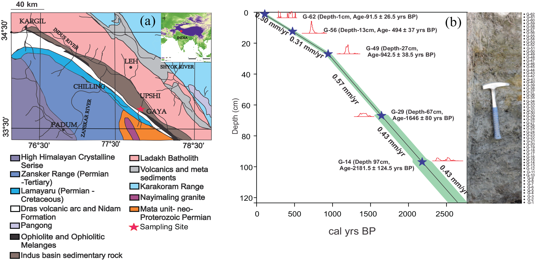
(a) SRTM image and Lithological map of the study area after Handerson et al. (2011); (b) the adopted age-depth model of the sediment section.

The catchment of Miru River lies on the south western edge of the Tibetan Plateau and is fed by the ISM, westerly driven snow, and glacial melt (Karim and Veizer, 2002). The river drains orthogonally, from south to north through meta-sediments of the Tanglang La Formation, the Tethyan sedimentaries, and the sedimentary rocks of the Indus–Tsangpo Suture Zone (ITSZ; Jain, 2014) (Figure 1a). The ITSZ is composed of calcareous flysch of the Lamayuru Formation of Triassic to Jurassic age, the volcanic Dras and Nidam Formations of Cretaceous flysch, Indus Basin Sedimentary Rocks of Paleogene, and ophiolitic mélanges representing the remains of the Tethys sea floor (Brookfield and Reynolds, 1981; Honegger et al., 1982). To the north of the ITSZ, the terrain is composed of the Ladakh Batholith containing intrusive tonalite and granodiorite, with bodies of igneous mafic complexes with radiometric ages that suggest intrusive phases at 120, 60–40, and 20 Ma (Brookfield and Reynolds, 1981; Honegger et al., 1982).

Climate of the region

Ladakh, a region having an average altitude greater than 3000 m a.s.l. is bound by the Karakoram ranges in the north and the Higher Himalaya and Pir Panjal ranges in the south. The study area, north of the Pir Panjal and the Higher Himalaya lies in the rain shadow zone of ISM and its general climate is characterized as a high-altitude desert receiving scanty rainfall of ~80 to 100 mm during the months of July and August. The region also receives moisture in form of winter snow, supplied from the Mediterranean region by the westerlies (Demske et al., 2009). Overall, climate of Ladakh region is cold with average surface temperature below −20°C in winter. Summers are characterized by moderate ambient temperatures of ~20°C during sunny days. The region often receives extreme rainfall owing to the interaction of high-altitude westerly jets with SW monsoon moisture laden wind streams causing flash floods (Hobley et al., 2012).

Modern vegetation in the region

Owing to prevailing cold and arid climate, the region has meager or almost nil forest cover. The narrow floodplains and exposed gravel bars along streams however, support diversified plant communities such as Asteraceae, Poaceae, Fabaceae, Astragulus, Polygonum, Potenilla, Brassicaceae, Artemisia, Rosa, Corydalis, Euphorbia, Calamagerosis, and tree species such as Salix, Juglans, Polulus, and Morus alba (Kala, 2011; Sagwal, 1991). From the Lesser Himalaya to the high ranges of Ladakh, the vegetation changes from temperate to desert type which can be observed from the drastic reduction of forest cover with rising altitude, resulting in substantial decrease in arboreal species in this region. The herbaceous species found in Ladakh are quite similar to those found in the Kashmir valley (Durani et al., 1975). The forest in the wetter monsoon dominated zone (south of the Higher Himalaya and Pir Panjal ranges) consists of dry alpine pastures with conifers and broad-leaved trees (Yadav et al., 2017). The conifers making the majority of the forest comprise chir (Pinus roxburghii Sarg.), kail (Pinus wallichiana A.B. Jacks), deodar (Cedrus deodara (Roxb.) G. Don), and silver fir (Abies pindrow (Royle ex D. Don) Royle), whereas the broad-leaved trees consist of Quercus leucotrichophora A. Camus ex Bahadur (banj oak), Q. floribunda Lindl. ex A Camus (Tilonj oak), Q. semicarpifolia Sm. (Kharsu), Mallotus philippinensis (Lam.) Muell. Arg., Acacia spp. (Acacia catechu (L. f.) P.J.H. Hurter & Mabb., A. modesta Wall), and Emblica officinalis Gaertn. (Quamar et al., 2018).

Methodology

Sampling, chronology, and age-depth model

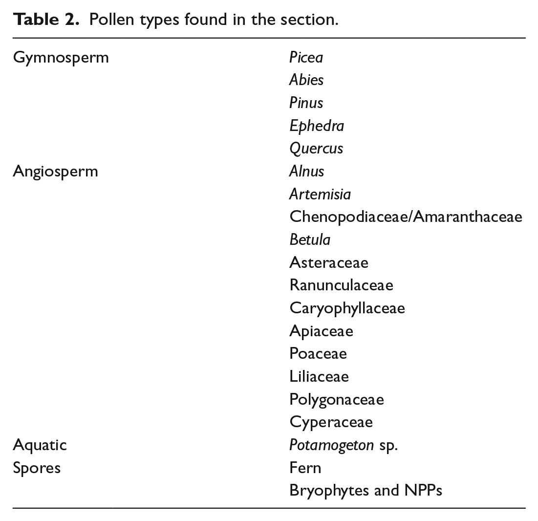
The sedimentary section was sampled at 2 cm interval and a total of 62 samples were collected and analyzed for a suite of biotic (pollen), abiotic (geochemical and environmental magnetic) proxies. Decalcification of sediment samples (treatment with 10% HCl) indicated negligible amount of inorganic carbonate throughout the section. Five samples rich in organic matter were selected for AMS ¹⁴C dating (Table 1). These aliquots were sent to the Poznan Radiocarbon Laboratory, Poland, for AMS ¹⁴C dating. Obtained radiocarbon ages were calibrated using CALIB Radiocarbon Calibration software (Calib 7.0.4; Reimer et al., 2013; Stuiver et al., 1998). All ¹⁴C dates are presented in Table 1 and are represented graphically with their probability distribution curves (red color, x-axis as age and y-axis as the frequency) (Figure 1b).

Table 1.

Sample details of ¹⁴C AMS dates.

Lab name	Depth (cm)	Sample type	¹⁴C AMS ages	Calibrated age (2σ cal. yr BP)	Calibrated error (years)	Depth interval (cm)	Sedimentation rate of the interval (mm/year)
Poz-85041	1	Bulk sediment	115.84 ± 0.32	91.5	26.5	1–11	0.30
Poz-85038	13	Bulk sediment	435 ± 30	494	37	11–25	0.31
Poz-85037	27	Bulk sediment	1020 ± 30	942.5	38.5	25–65	0.57
Poz-85036	67	Bulk sediment	1750 ± 30	1646	80	65–95	0.43
Poz-85034	97	Bulk sediment	2160 ± 30	2181.5	124.5	95–124	0.43

AMS: accelerator mass spectrometry.

Pollen analysis

Pollen analysis was carried out on alternate samples, that is, a total of 31 samples were analyzed. Sample processing involves addition of Lycopodium marker spores (~10,680 spores per tablet) in 2 g sediment of each sample for the estimation of pollen concentration (Stockmarr, 1971) followed by sequential pretreatment with HCl, HF, and KOH in order to remove carbonates, silicates, and organic matter, respectively (Moore et al., 1991). Recovered sediments were then sieved on 10 µm mesh, for the removal of material other than pollen/spore grains. The final pollen residue was stained with Safranin ‘O’ and slides were prepared for microscopic study. Olympus BX 61 transmitted light microscope was used for pollen counting and identification. Identification of pollen and spores was aided by published literature and standard keys (Erdtman, 1943; Gupta and Sharma, 1986; Moore et al., 1991; Moore and Webb, 1978; Punt et al., 2007). A minimum of ~300 terrestrial pollen grains were counted in each sample. Pollen zonation utilized Tilia software (version 2.1.1) cluster analysis Constrained Instrumental Sum of Squares (CONISS; Grimm, 1987). Pollen concentration of each sample was estimated using the formula – ‘{(pollen grains counted/marker grains counted) × 10,680 / weight of sediment}’.

Environmental magnetism

Magnetic parameters such as χlf, ARM (anhysteretic remnant magnetization), and IRM (isothermal remnant magnetization) were measured at Paleomagnetic laboratory, Wadia Institute of Himalaya Geology, Dehradun. Dry homogenized samples were packed in a 10-cm³ nonmagnetic styrene container. The bulk magnetic susceptibility in low (κlf) and high (κhf) frequencies were measured in all six directions and the mean of average κlf and κhf were divided by sample weight to get χlf and χhf. The χlf and χhf represent mass specific average susceptibility of all six directions at 0.46 kHz (low frequency) and 4.6 kHz (high frequency), respectively. ARM was measured by placing each sample in a peak alternating field of 100 mT in a DC field of 0.1 mT using Molspin Alternating Field Demagnetizer (UK). IRM was measured using forward incremental fields at 50, 100, 300, 500, 600, 800, 1000, 1200 mT and backward fields at −10, −20, −30, −50, −100, −300, −400 mT using impulse magnetizer. Instrumental parameters such as B_cr (coercivity of remanence), SIRM (saturated isothermal remnant magnetization), S-Ratio (ratio of high-coercivity minerals with respect to low-coercivity minerals), and χARM (mass-specific ARM) were also calculated. B_cr is the amount of magnetic field required to bring down a material to zero magnetization from saturation by applying reverse field and is used to determine the concentration of minerals such as hematite and goethite. SIRM is used to determine the concentration of the type of magnetic minerals by observing its magnetic saturation. S-Ratio is used to measure the abundance of high coercivity minerals. χARM measures the ability to retain a magnetic remanence which is a function of the abundance of fine grained SSD (stable single domain)/SD (single domain) magnetic particles as well as the concentration of magnetic minerals (Liu et al., 2012).

TOC, TN, and stable isotopic composition (δ¹³C, δ¹⁵N)

All 62 samples were analyzed to measure TOC, TN contents, and their stable isotopic ratios. For this, we used Elemental Analyzer (EA; Vario Isotope Select; Elementar, Germany) coupled with Isotope Ratio Mass Spectrometer (IRMS; Isoprime Precision; Elementar, UK) in continuous flow mode, an analytical facility established recently at Birbal Sahni Institute of Palaeosciences, Lucknow. Sediment samples were first dried, powdered, and then again dried in an oven at 50°C. An amount of ~10 mg of sample sizes were weighed in tin boats and packed in oval shape pellets. Pellets were pressed from all the sides to remove air to ensure that measured δ¹⁵N is unaffected by isotopic composition (N₂) of air. Packed tin boats were dropped into the combustion reactor of EA containing copper oxide as catalyst and heated at 950°C to carry out flash combustion of samples in the presence of high purity oxygen gas (O₂) (5-grade). The evolved gases from combustion reactor were passed through a reduction reactor containing reduced copper at 550°C ensuring that oxides of nitrogen (NOx) were converted to N₂ gas for reliable isotopic composition data of sample N. Gas streams were then further passed through a moisture-trap tube filled with P₂O₅ (Sicapent) to ensure the complete removal of moisture. Dry Helium gas (purity: 99.999%) was used as the carrier gas. Purified CO₂ and N₂ were further separated using a chromatographic column and then passed through a thermal conductivity detector (TCD) for their quantification. Analytes, CO₂, and N₂ were then passed to IRMS sequentially for isotopic measurements. Sample analyte gases (CO₂ and N₂) were measured with reference to the gases CO₂ and N₂ (purity: 99.999%). The C and N contents and their isotopic values were calibrated against a suite of international (International Atomic Energy Agency (IAEA)) and in-house synthetic as well as sedimentary standards. For determining organic carbon content sediment samples were decalcified using 10% HCl, washed thoroughly with deionized water to remove any excess of chloride ions, and then dried and decalcified powders were used for determining TOC contents and δ¹³C_org as described. It should be noted that TN contents and δ¹⁵N were measured in the dried bulk fraction only. Overall, uncertainty with TOC and TN contents were better than 3–5% and overall uncertainty of isotopic data are within 0.2‰.

Results

Lithosection, adopted chronological model and temporal resolution

The entire 1.23-m-thick sedimentary (Upshi) section is composed of three distinct sedimentary units showing faint bedding structures and low degree of bioturbation. The bottom most unit (123–69 cm depth) appears to be composed of black clayey silt with sporadic pebbles. This sequence is overlain by a ~30-cm-thick (69- to 40-cm-depth) yellow clayey silt unit showing extensive iron oxidation. The topmost unit (40–0 cm depth) is composed of grayish yellow clayey silt (Figure 1b). Samples selected for AMS ¹⁴C dating were obtained from the depth intervals of 1–3 cm, 13–15 cm, 27–29 cm, 67–69 cm, and 97–99 cm. Calibrated ages of these horizons are shown in Table 1 and Figure 1b. The section exhibited varying sedimentation rates ranging from ~0.30 to 0.57 mm yr⁻¹. The oldest estimated age of the bottom most sample is 2646 ± 125 years, whereas the youngest uppermost layer of the section is 92 ± 27 years. Estimated average temporal resolution from the studied section is ~43 years.

Palynology

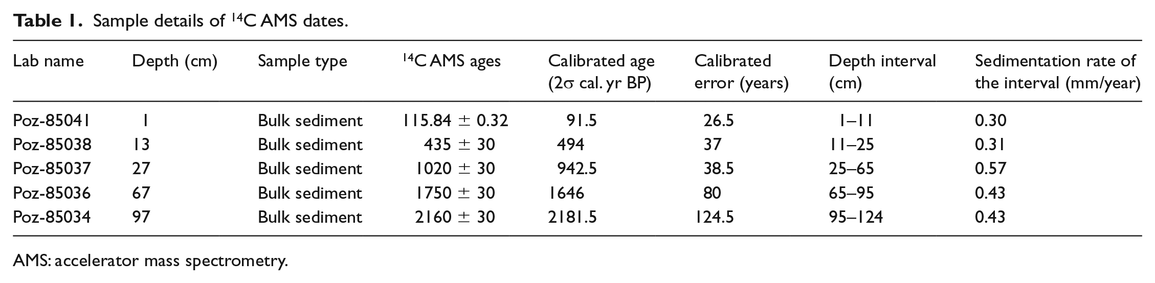
Details of palynomorphs recovered from the Upshi section are given in Table 2. Arboreal pollen (AP) is mainly represented by conifers (Pinus, Abies, and Picea) and broad-leaved trees (Quercus, Betula, and Alnus). The recovery of AP from the sedimentary sequence reflects long-distance aeolian transportation from down valley forests. The non-arboreal pollen (NAP) is composed of Ephedra spp., Chenopodiaceae/Amaranthaceae (Cheno/Am), Liliaceae, Umbelliferae, and so on. Occurrence of grasses (Cyperaceae and Poaceae) and aquatic taxa (Potamogeton sp.) are also noted (Figure 2). The pollen percentage diagram, as plotted, refers to total pollen sum of terrestrial pollen taxa (100%). Pollen percentages were calculated for taxa accounting >0.5% of the total pollen grains in at least three samples. To avoid the over-representation of some plants in pollen spectra taxa like Cyperaceae, Poaceae, aquatic plants and ferns are excluded from the total pollen sum and are presented in concentration per gram (grains/g) (Figure 3). Pollen biostratigraphy is achieved by division into three major pollen zones (PZ 1–3) based mainly on the CONISS cluster analysis results (using Tilia 2.1.1 program; Grimm, 1993) and changes in terrestrial pollen percentages (Figure 3). The paleofloristic description of each PZ is described as follows:

Table 2.

Pollen types found in the section.

Gymnosperm	Picea
	Abies
	Pinus
	Ephedra
	Quercus
Angiosperm	Alnus
	Artemisia
	Chenopodiaceae/Amaranthaceae
	Betula
	Asteraceae
	Ranunculaceae
	Caryophyllaceae
	Apiaceae
	Poaceae
	Liliaceae
	Polygonaceae
	Cyperaceae
Aquatic	Potamogeton sp.
Spores	Fern
Spores	Bryophytes and NPPs

Figure 2.

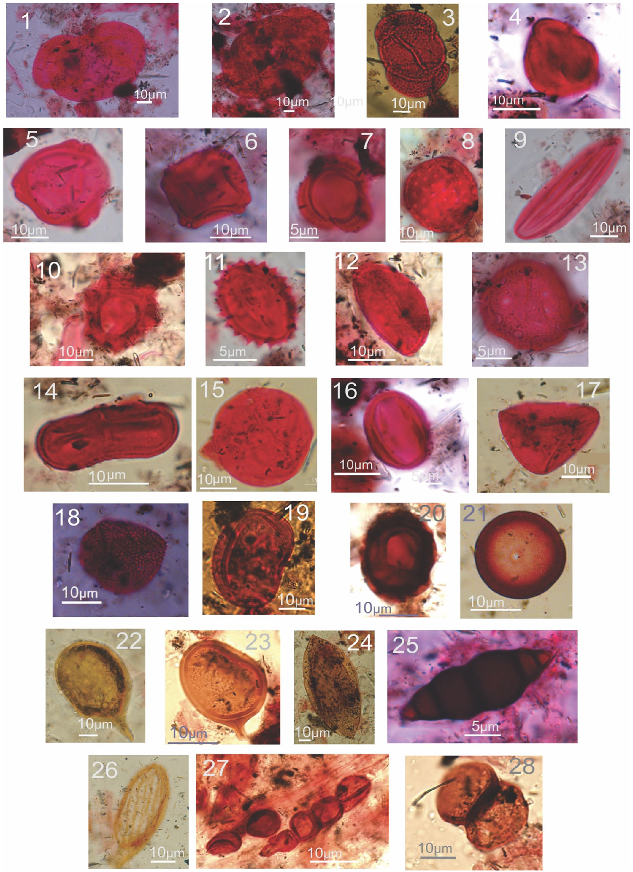
Pollen and NPP (non-pollen palynomorphs) photographs: 1. Picea, 2. Abies, 3. Pinus, 4. Quercus, 5. Betula, 6. Alnus, 7. Artemisia, 8. Chenopodiaceae, 9. Ephedra sp., 10–11. Compositae (Liguliflorae and Tubiliflorae), 12. Ranunculaceae, 13. Caryophyllaceae, 14. Apiaceae, 15. Poaceae, 16. Polygonaceae, 17. Cyperaceae, 18. Potamogeton sp., 19. Polypodiaceae, 20–28. NPP.

Figure 3.

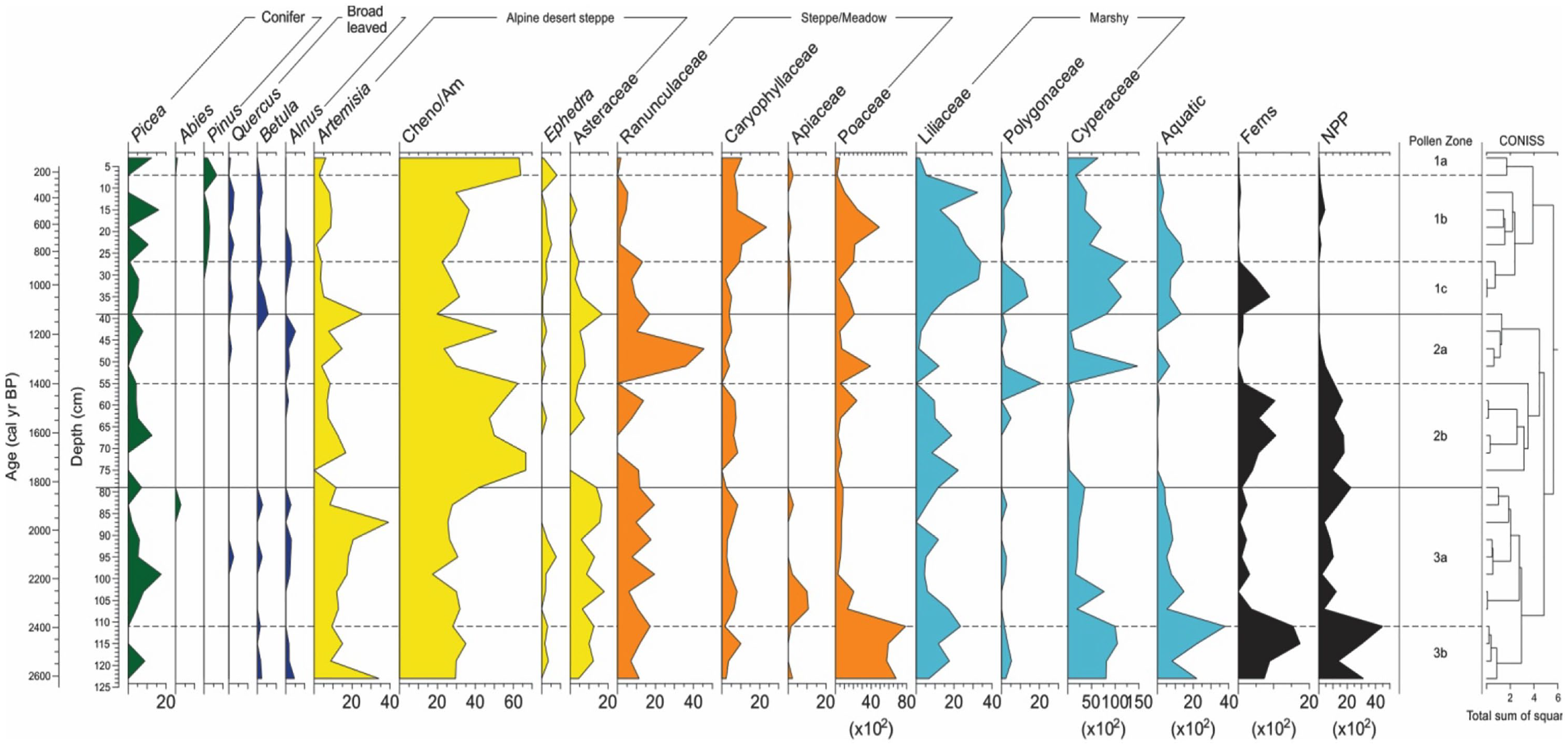
Pollen diagram of Upshi–Gaya section shown on the basis of concentration of the different types of pollen. Zones are marked with solid horizontal lines and subzones by dotted horizontal lines.

PZ-3 (~2646 to 1860 cal. yr BP; 123–79 cm)

This zone is characterized by the dominance of NAP over AP. The NAP includes Artemisia, Poaceae, Ranunculaceae, Asteraceae, Cyperaceae, aquatic plants, non-pollen palynomorphs (NPP), and tree taxa such as Abies, Pinus, and Quercus. This zone is divided into two subzones (PZ 3b and 3a).

PZ-3b (~2646 to 2431 cal. yr BP; 123–111 cm) is marked by high frequencies of herbaceous taxa such as alpine desert steppe (~53% to 68%); marshy taxa like Liliaceae (~23%), Polygonaceae (~7% to 23%); Cyperaceae (800–1000 grains/g), and NPP (300 grains/g). This zone records the highest number of NPP (140–450 grains/gm) in the entire profile. Fern spores (monolete) shows increasing trend from the bottom (70–150 grains/g). However, among conifers only Picea (9%) is present at 119-cm-depth interval, whereas broad-leaved taxa Betula (~2%) and Alnus (2–5%) are recorded in good number. Aquatic pollen taxa (57–79 grains/gm) are present in high concentration.

PZ-3a (~2431 to 1860 cal. yr BP; 111–79 cm) shows mixed broad-leaved and conifer forest in the region. Broad-leaved tree taxa show an average of ~3% while conifers have an average of ~7% pollen. This zone is mostly dominated by the alpine desert steppe and other local meadow plant taxa. Among NAP the highest percentages is of alpine desert steppe (average ~60%) among which pollens of Cheno/Am, Artemisia, and Asteraceae are recorded to be 29%, 17%, and 12%, respectively. Other dominant plants include Ranunculaceae (13%) and Liliaceae (8%). Pollen grains of sedges and grasses and spores of ferns (bryophytes and fungal) are reported in lower concentrations than the previous subzone. The highest percentage of Umbelliferae in the pollen spectrum is recorded in this subzone.

PZ-2 (~1860 to 1154 cal. yr BP; 79–39 cm)

In this zone, there is conspicuous absence of AP except Picea and significantly reduced NAP. The broad-leaved taxa (Betula and Alnus) appear only after ~1400 cal. yr BP at ~60 cm depth. High influx of alpine desert steppe taxa mostly dominated by Cheno/Am is followed by Artemisia and Asteraceae. NPP spores (bryophytic, algal, and fungal) shows increased abundance. Except for Liliaceae other herbaceous taxa show reduced pollen percentage. Overall, PZ-2 is marked by climatic deterioration with slightly improved wetter conditions after ~1400 cal. yr BP. This zone is divided into two subzones:

PZ-2b (~1860 to 1435 cal. yr BP; 79–55 cm) is dominated by Cheno/Am (58%) and NPP (140 grains/g). Among arboreal taxa, only Picea (4%) is recovered.

PZ-2a (~1435 to 1154 cal. yr BP; 55–39 cm) shows a gradual increase in Betula (1%), Alnus (2%), and Quercus (1%). The contribution of Cheno/Am (31%) is the highest followed by Ranunculaceae (27%) and Artemisia (13%). Relatively high concentration of Cyperaceae (620 grains/g) and Poaceae (180 grains/g) is recorded here, whereas NPP concentration has decreased substantially from subzone 2b (140 grains/g) to subzone 2a (200 grains/g).

PZ-1 (1154 cal. yr BP to present; 39–0 cm)

This zone is subdivided into three subzones, and is dominated by the mixed broad-leaved trees, conifer forest, and herbaceous taxa of Caryophyllaceae, Liliaceae, Cyperaceae, and aquatic pollen.

PZ-1c (~1154 to 943 cal. yr BP; 39–27 cm) demonstrates mixed broad-leaved and conifer forest. High frequency of diverse pollen taxa of Ranunculaceae, Polygonaceae, Liliaceae, and Cyperaceae are visible. Increased aquatic and fern taxa imply augmented precipitation.

PZ-1b (~943 to 293 cal. yr BP; 27–7 cm) is characterized by relatively denser mixed broad-leaved and conifer forest than the previous subzone. Conifers (9%) dominate over the broad-leaved taxa (7%). Cheno/Am increases toward the upper subzone boundary. Caryophyllaceae, Poaceae, Liliaceae, and Cyperaceae are present in good number but shows a decreasing trend.

PZ-1a (Since ~293 cal. yr BP; 7–0 cm depth) except Cheno/Am meadow elements are sporadically present. Pollen of Artemisia, Cyperaceae, Caryophyllaceae, Picea and Pinus are present in moderate number. Fern spores are absent.

Sedimentary TOC, TN contents, and stable isotopes (δ¹³C, δ¹⁵N)

TOC (wt%) in the Upshi section varies between a minimum of 0.48% and a maximum of 6% with an average value of 2.7%. The TN varies up to 0.48% with an average of 0.22%. The δ¹³C value of C_org component shows variation from a maximum of −19‰ to a minimum of −25.8‰. δ¹⁵N values in the section show variation between 0.9‰ and 8.2‰ with an average of 4.9‰ (Table 3).

Table 3.

Data for TOC, TN, δ¹³C_org, and δ¹⁵N.

Sample no.	TOC (%)	TN (%)	δ¹³C_org (‰)	δ¹⁵N (‰)
G-1	2.13	0.07	−22.7	5.0
G-2	1.39	0.08	−22.7	4.5
G-3	1.67	0.12	−22.1	4.7
G-4	1.97	0.12	−22.6	4.4
G-5	4.24	0.20	−21.8	4.6
G-6	2.65	0.15	−24.9	5.4
G-7	3.27	0.21	−23.6	5.7
G-8	3.22	0.22	−24.4	5.1
G-9	2.34	0.13	−24.1	2.8
G-10	0.53	0.01	−23.8	0.9
G-11	0.48	0.09	−21.4	4.1
G-12	0.96	0.04	−24.5	3.7
G-13	1.09	0.02	−25.6	2.9
G-14	0.22	0.00	−23.9	4.4
G-15	0.65	0.03	−22.6	4.2
G-16	3.11	0.02	−24.0	5.4
G-17	1.45	0.03	−24.4	4.2
G-18	1.79	0.10	−25.2	4.6
G-19	1.82	0.08	−24.9	4.4
G-20	3.72	0.16	−24.0	5.3
G-21	1.40	0.07	−25.2	5.4
G-22	1.20	0.18	−25.2	5.5
G-23	2.19	0.13	−25.0	5.7
G-24	2.39	0.12	−25.3	5.9
G-25	1.95	0.13	−25.8	5.1
G-26	2.23	0.16	−25.8	6.4
G-27	2.72	0.17	−24.0	5.3
G-28	3.25	0.22	−25.2	5.4
G-29	2.29	0.12	−25.2	5.5
G-30	1.91	0.09	−25.0	5.7
G-31	1.90	0.07	−25.3	5.9
G-32	3.42	0.10	−25.8	5.1
G-33	2.72	0.08	−25.8	6.4
G-34	3.87	0.41	−26.3	5.0
G-35	4.81	0.48	−26.5	5.3
G-36	5.27	0.47	−26.0	5.5
G-37	2.36	0.30	−25.4	4.7
G-38	1.86	0.25	−24.9	3.8
G-39	1.09	0.20	−24.5	2.0
G-40	1.19	0.21	−24.5	3.9
G-41	1.73	0.18	−24.5	1.2
G-42	1.72	0.15	−24.2	1.6
G-43	2.87	0.24	−24.8	3.3
G-44	4.86	0.32	−25.1	3.9
G-45	5.47	0.52	−25.4	5.3
G-46	5.61	0.51	−25.6	3.7
G-47	3.84	0.37	−25.4	4.8
G-48	3.91	0.43	−26.3	3.9
G-49	3.98	0.35	−26.6	4.7
G-50	3.95	0.32	−25.9	4.5
G-51	1.94	0.28	−24.5	4.8
G-52	3.20	0.41	−20.8	6.7
G-53	4.51	0.32	−22.0	5.3
G-54	5.91	0.51	−19.8	6.8
G-55	5.59	0.48	−20.0	6.8
G-56	5.21	0.41	−19.9	6.9
G-57	4.87	0.26	−21.8	6.0
G-58	2.98	0.39	−19.6	6.9
G-59	6.00	0.53	−19.0	8.2
G-60	2.53	0.20	−19.2	4.1
G-61	3.60	0.39	−20.1	5.7
G-62	5.09	0.42	−19.3	6.1

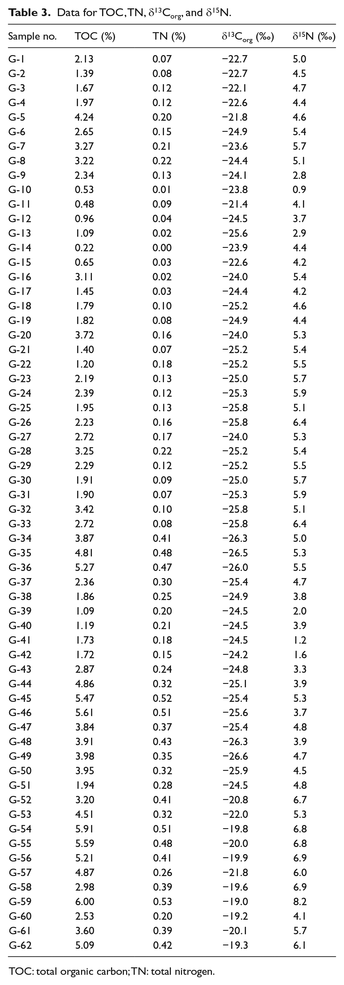
TOC: total organic carbon; TN: total nitrogen.

Environmental magnetism

Magnetic parameters were measured in all 62 samples (Table 4). Inter-parametric scatter graph of magnetic data are shown in Figure 4. Significant correlations are observed between χARM and χlf; SIRM and χlf; B_cr and S-Ratio; δ¹³C and B_cr; δ¹⁵N and B_cr (Figure 4a–e) with R² values ~0.78, 0.74, 0.75, 0.43, and 0.31, respectively. Correlation of χlf and χARM indicates that increased concentration of magnetic susceptibility is linked to SP (super paramagnetic)/SD size particles (Buggle et al., 2014; Rawat et al., 2015b). Correlation of χlf and SIRM suggests little change in magnetic grains that contribute to bulk susceptibility (Liu et al., 2004). Control of magnetic hard minerals such as hematite and goethite with increase in coercivity is also inferred from Figure 4c, where correlation of B_cr and S-Ratio holds well (p = 0.75). Figure 4d and e shows isotopes of C and N are linked with coercivity parameter (B_cr). All these indicate that χlf is controlled by concentration of fine grained SSD (stable single domain)/SD particles with lower coercivity (Egli and Lowrie, 2002; Eyre, 1997; Liu et al., 2012; Lu et al., 2010). The χlf values vary between 0.77 and 1.91 (10⁻³ m³ kg⁻¹) with mean value of 1.1 (10⁻³ m³ kg⁻¹).

Table 4.

Environmental magnetic data.

Sample no.	χlf (10⁻⁸ m³ kg⁻¹)	χARM (10⁻⁸ m³ kg⁻¹)	SIRM (10⁻⁵ A kg⁻¹)	S-Ratio	B_cr
G-1	1.32960199	0.024375609	123.5	−0.850927548	44
G-2	0.982716049	0.008933557	94.11851852	−0.934833937	44
G-3	1.049613563	0.026215596	141.0695587	−0.963893749	40
G-4	1.034883721	0.027462896	146.6666667	−0.962896406	41
G-5	0.997484277	0.028064853	136.5358491	−1.004035156	40
G-6	0.976738039	0.017932645	84.56780333	−0.906507877	39
G-7	1.31697487	0.022963323	89.76529161	−0.986292687	35
G-8	1.05277329	0.012075726	45.99353796	−0.967334036	35
G-9	1.005221932	0.034003787	73.16797215	−0.968478649	38
G-10	1.031483928	0.013774288	65	−0.939538665	40
G-11	0.820430108	0.007213487	32.34193548	−0.783163774	44
G-12	0.782152231	0.018498002	81.55905512	−0.940625603	38
G-13	0.95221765	0.011115247	43.45679012	−0.90625	40
G-14	0.824742268	0.008720579	35.44329897	−0.927089393	39
G-15	1.211474633	0.033506794	153.9544808	−1.007668853	40
G-16	1.258461538	0.049014302	251.7538462	−1.033243706	44
G-17	1.227147508	0.033884675	193.5386927	−1.013975155	36
G-18	1.100737667	0.021459302	86.7219917	−1.012759171	34
G-19	1.313649979	0.033221306	206.1617458	−1.009339975	43
G-20	1.634482759	0.06290071	327.7241379	−0.99263468	40
G-21	1.911371581	0.06277532	328.1924738	−0.99924812	50
G-22	1.692922374	0.031234942	215.890411	−1.00285533	56
G-23	1.395850175	0.021530449	120.9377526	−0.92473262	46
G-24	1.434886499	0.004052521	114.5519713	−0.942803504	52
G-25	1.022635408	0.005484171	20.78415521	−0.684947491	37
G-26	1.518672199	0.00510853	24.14937759	−0.8	17
G-27	1.221470837	0.004991143	17.49788673	−0.698550725	30
G-28	1.338383838	0.005829336	22.91666667	−0.745454545	23
G-29	0.904761905	0.004645074	15.93277311	−0.65242616	48
G-30	0.962187711	0.004750288	17.12356516	−0.72555205	50
G-31	0.797886053	0.00476085	18.56921887	−0.802165764	53
G-32	0.832159624	0.00504282	18.70422535	−0.792921687	52
G-33	0.824039653	0.004296576	15.44981413	−0.768046198	51
G-34	0.769607843	0.00357178	11.04901961	−0.702750665	45
G-35	0.824175824	0.003623889	12.9532967	−0.835630965	29
G-36	0.912022704	0.003403239	9.829721362	−0.611023622	49
G-37	0.979381443	0.003145329	11.57584683	−0.519083969	66
G-38	0.915422886	0.002718818	10.79104478	−0.415629322	105
G-39	0.877642537	0.002897254	11.27482383	−0.504545455	68
G-40	0.857981959	0.003162445	10.22655758	−0.497230769	80
G-41	0.780538302	0.003745435	12.20496894	−0.552671756	60
G-42	0.81300813	0.003992616	12.88987435	−0.525229358	63
G-43	0.931263858	0.003064101	12.6977088	−0.541909197	65
G-44	0.934430965	0.003919075	11.94107452	−0.563134978	53
G-45	0.909346847	0.003925879	10.92905405	−0.5	70
G-46	0.939745716	0.003750094	13.08457711	−0.391001267	72
G-47	0.866551127	0.003483623	11.17850953	−0.356589147	80
G-48	0.802524797	0.003171856	10.27953111	−0.362280702	74
G-49	0.796547821	0.00362594	10	−0.447368421	62
G-50	0.999455338	0.004823956	12.46732026	−0.442988204	57
G-51	0.86163522	0.005499194	16.09811321	−0.476324426	43
G-52	0.886623417	0.006287229	16.73772011	−0.478405316	40
G-53	1.146968427	0.028432186	52.41408215	−0.726211419	7
G-54	1.113680154	0.029150708	50.23947151	−0.73339908	9
G-55	1.131215063	0.031711958	53.99823477	−0.76822491	4
G-56	1.529892837	0.025295683	50.10152284	−0.787234043	12
G-57	1.095666394	0.02383134	45.64186427	−0.738086707	9
G-58	0.951029099	0.139091483	28.85734564	−0.622233153	21
G-59	1.399214264	0.047153264	78.4950136	−0.780780781	4
G-60	0.863821138	0.012256404	34.45121951	−0.637168142	20
G-61	1.049204052	0.013453665	36.85962373	−0.610129564	26
G-62	1.465661642	0.036404805	71.74204355	−0.766051833	11

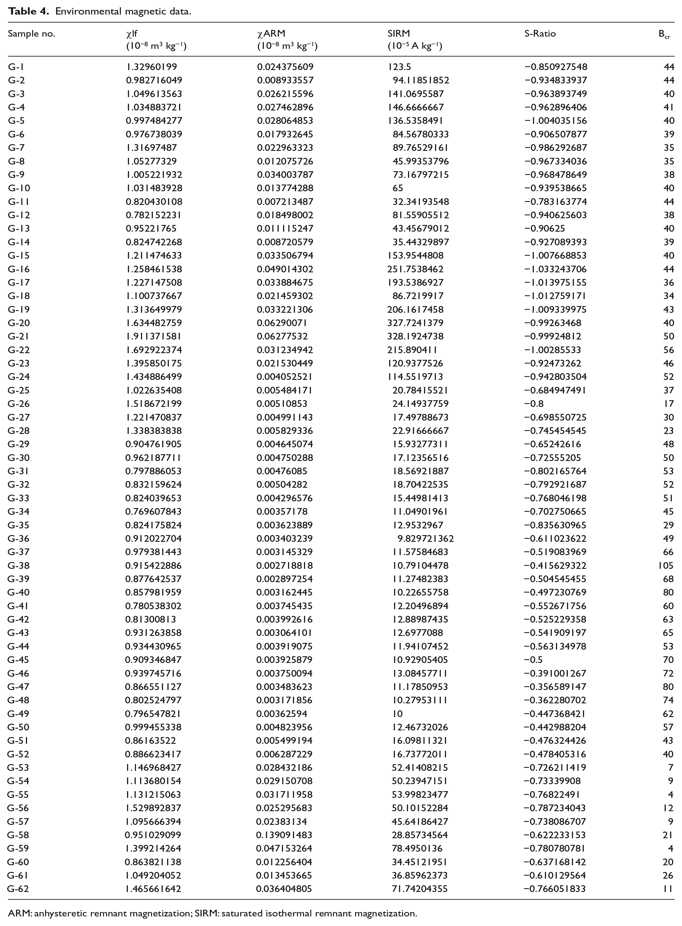
ARM: anhysteretic remnant magnetization; SIRM: saturated isothermal remnant magnetization.

Figure 4.

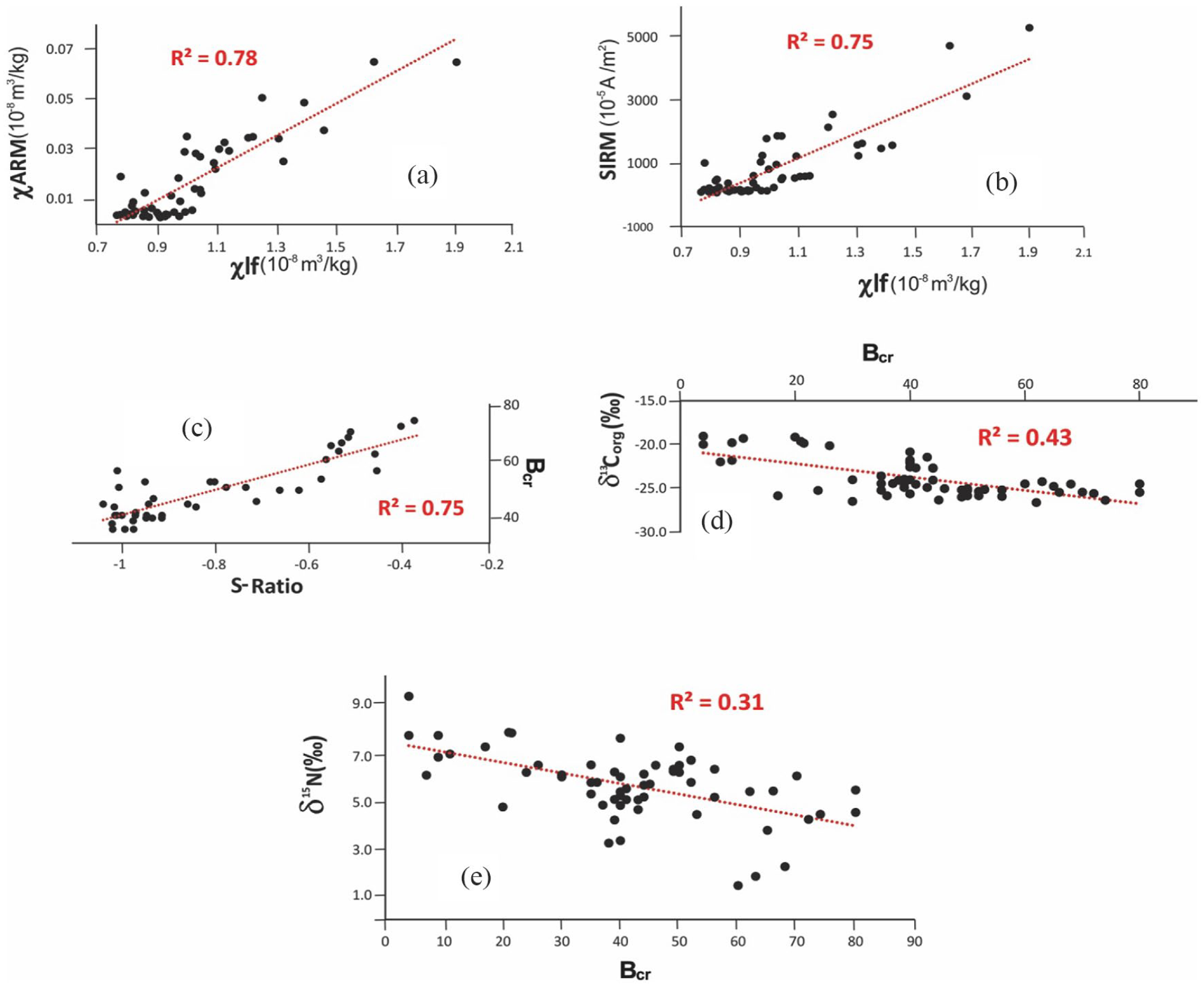
Scatter plots of magnetic parameters and δ¹³C_org, δ¹⁵N: (a) χlf vs χARM, (b) χlf vs SIRM, (c) S-Ratio vs B_cr, (d) B_cr vs δ¹³C_org, and (e) B_cr vs δ¹⁵N.

Proxy response to climate (monsoonal) change

This study attempts to reconstruct the monsoonal variability from a ~2700-year-long sediment record using multiple proxies – pollen, TOC, TN, stable isotopes (δ¹³C, δ¹⁵N), and environmental magnetism. The pollen study is focused on understanding changes of the vegetation pattern during the past ~2700 years in response to the ISM. High contribution of conifer and broad-leaved AP from the profile indicates intense wind activity facilitating uphill transportation of pollen grains from wetter lower elevations which may suggest stronger ISM (Rawat et al., 2015a). Xerophytes, represented in the record by Cheno/Am, Artemisia, and Ephedra commonly grow in arid regions. NPP (algal and fungal spores) suggest hostile conditions with reduced moisture implying drier conditions. Algal spores can also indicate the decomposition of organic material in dry conditions (Van Geel, 1986). The high frequency of fungal hyphae implies increased dryness (Eisner and Peterson, 1998). Abundance of ferns in contrast suggests moist and damp environment around the study area.

Concentrations of TOC and TN (wt%) in the studied section are expected to mimic biogenic soil organic productivity. Hence, TOC and TN are expected to be enhanced (decreased) with higher wetness/ monsoonal activity (drier and colder) periods (Srivastava et al., 2017b). Warmer temperatures in the region would introduce more moisture in surface soils due to melting of snow making surface soil conducive for bacterial activities and for the growth of diverse vegetation. However, surface biogenic productivity could be limited by nutrient availability in higher reaches of the Himalaya as reported from a peat record of Garhwal Himalaya (Srivastava et al., 2017b). A statistically sound correlation between TOC and TN (wt%; Pearson correlation r² = 0.7; n = 62; p< 0.01) indicates both components were deposited in this wetland and also suggests better preservation conditions of biogenic proxies in the studied section with minimal influence of post deposition digenesis (see Figure 5a).

Figure 5.

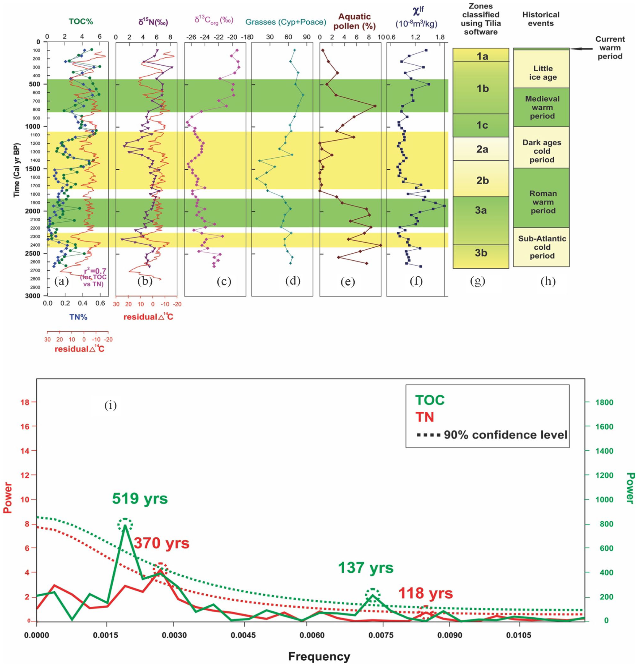
(a) TOC, TN, and residual Δ¹⁴C; (b) δ¹⁵N and residual Δ¹⁴C; (c) δ¹³C_org; (d) grasses (Cyperaceae + Poaceae); (e) aquatic pollen; (f) χlf; (g) pollen zones green and yellow represents wet and dry phases, respectively; (h) global climatic and major historical events linked with climate change; and (i) spectral analysis of TOC (total organic carbon) and TN (total nitrogen) time series of Upshi–Gaya section showing periodicities of 519, 370, 137, and 118 years (oversample size, 1; number of segments, 1) at 90% confidence level using Past 3.20.

In high-altitude regions like Ladakh, carbon sequestration could be driven by the photosynthetic capability of soil and channelized through atmospheric N fixation (Srivastava et al., 2017b). Observed range of δ¹⁵N values and correlative analysis (Pearson’s correlation coefficient between TN and TOC with δ¹⁵N) do not indicate atmospheric N deposition during high carbon capture (sequestration) period for this wetland area (Figure 5b). Hence, sedimentary δ¹⁵N values would mimic changes in soil N type only. This inference is further reinforced by the depth profile of δ¹³C_org, which does not show any significant correlation with TOC or TN indicating surface soil δ¹³C_org or δ¹⁵N values are not influenced by any soil-sedimentary biogeochemical changes. Besides significant correlation that exists between δ¹³C_org and pollen counts (Cyperaceae + Poaceae; shown later as Figure 5c and d) strongly corroborates our earlier-mentioned contention.

Examining the interrelationship between TN (and TOC) content and δ¹⁵N indicate that enriched δ¹⁵N values largely occurred during high TN (and TOC) periods (Figure 5a and b) and this indicates a plausible subsurface water column denitrification in wetlands during warmer and wetter phases. Hence during long wetter phases, higher surface biogenic productivity induced by available nutrients ( $N O_{3}^{-}$ and ${NH}_{4}^{+}$ ) may invoke water column denitrification and this phenomenon might be captured in the sediment column by enriched δ¹⁵N values. In contrast, colder and drier periods could be characterized by lower δ¹⁵N values (see Figure 5b). However as stated earlier, TN-δ¹⁵N plot show no evidence of surface N uptake through atmospheric fixation. This indicates that surface soil in the region has remained devoid of N-fixing bacteria (diazotrophs) during its depositional history (~last 2700 years).

δ¹³C_org values of TOC primarily indicate vegetation type (C₃, C₄, or CAM). The C₃ plants exhibits a range of carbon isotope composition from −34‰ to −24‰ (Vienna Pee Dee Belemnite [V-PDB]) with an average of −27‰, whereas C₄ plants ranges from −17‰ to −9‰ (V-PDB) with an average value of −13‰. In this high-altitude region, δ¹³C of TOC could be affected by several environmental factors such as the temperature, relative humidity, altitude, vegetation, and the concentration of CO₂ in the atmosphere (Srivastava et al., 2017b; Zhong et al., 2017). However, a striking similarity seen in the depth profile of δ¹³C of TOC and pollen record grasses (Figure 5c and d) suggesting that here δ¹³C_org values of sedimentary layers mimic surface vegetation changes and characteristically capture a wetter phase commencing on ~800 cal. yr BP (Figure 5c), which is well supported by the increase of aquatic pollen taxa during this period (Figure 5e). Comparison of TOC, TN, δ¹⁵N, and residual Δ¹⁴C, together with spectral analysis of TOC and TN data hints a dominant influence of solar forcing (Figure 5a, b, and i).

Magnetic susceptibility (χlf) has been used as an interesting proxy for reconstructing monsoonal intensity during the Holocene in geological repositories of the Higher Himalaya (Srivastava et al., 2013, 2017b). It increases with increasing concentration of magnetizable minerals at the deposition site. This would happen during increased supply of iron bearing detrital minerals through freezing and thawing conditions under dry and cold climate and vice versa. In addition, the values of sedimentary magnetic susceptibility (χlf) could also be affected by iron produced in situ as result of chemical weathering under warm and humid conditions. A careful inspection of rising trends in χlf, χARM, and the fall of S-Ratio and B_cr (Figure 6a–d) suggest higher concentrations of magnetic material in the sedimentary column are produced pedogenically under warm and humid climate (Figure 4; Liu et al., 2010). This is also comparable with the rise of δ¹³C_org and δ¹⁵N (Figure 6e and f). Pedogenesis enhances susceptibility (χlf) by increasing the concentration of magnetic minerals (e.g. magnetite) and SD/SSD particles. Rise of S-Ratio and B_cr being comparable to the fall of χlf implies reduction of low coercivity minerals such as magnetite and increase in goethite content. Hence, in our study we suggest that increase in the sediment χlf value is indicative of warmer and wetter conditions and the decrease is indicative of colder and drier conditions in the area.

Figure 6.

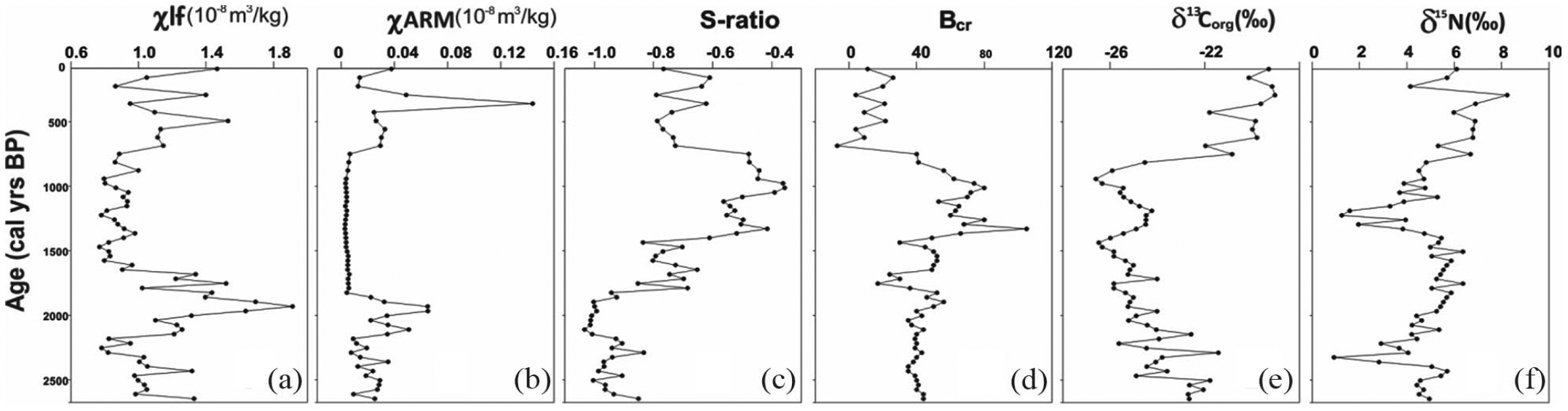
Plots of various magnetic parameters w.r.t. ages: (a) χlf, (b) χARM, (c) S-Ratio, (d) B_cr, (e) δ¹³C_org, and (f) δ¹⁵N.

Climatic history, regional correlations, and forcing factors

Climate variability in the region is inferred using (1) pollen assemblages and sedimentary δ¹³C for vegetation changes, (2) TOC, TN contents along with δ¹⁵N for biogeochemical changes in the sedimentary column, and (3) mineral magnetic susceptibility (χlf) also for wetness index as iron bearing minerals are sensitive to prevailing monsoonal changes. Sensitivities of these proxies to same climate forcing could be different temporally (Battarbee et al., 2002), however, for the deposition period, that is, for the past ~2700 years we do not anticipate this as a likely situation. Surface soil biogenic productivity indicators, TOC and TN which show robust inter-correlations throughout suggest these proxies indicate ambient wetter (warmer)/colder (drier) conditions rather well on subcentennial timescale. To evaluate the primary forcing behind the aforementioned quasi-cyclic biogeochemical changes in the sedimentary column, we plotted TOC and TN together with atmospheric Δ¹⁴C (residual) anomalies with respect to calibrated ages in Figure 5a as mentioned earlier. It can be seen that almost all the negative Δ¹⁴C excursion are coeval with higher TOC/TN, δ¹⁵N, and all the positive excursion fall with reduced TOC/TN, δ¹⁵N contents (Figure 5a and b). It should be noted that atmospheric Δ¹⁴C (residual) anomaly is used as an index of solar (intrinsic) variability (Agnihotri et al., 2002, 2011; Gupta et al., 2005), that is, negative residual Δ¹⁴C excursions are found during high solar activity, whereas positive residual Δ¹⁴C excursions indicate solar minima. Spectral analysis of TOC and TN shows periodicities of 519, 370, 137, and 118 years (Figure 5i). Previous studies from the Himalaya and the Arabian Sea (Agnihotri and Dutta, 2003; Agnihotri et al., 2002, 2011; Bhattacharyya and Narasimha, 2005; Gupta et al., 2005; Srivastava et al., 2013, 2017b) have demonstrated that ISM intensity fluctuates with solar variability on decadal to centennial timescale and the ISM enhances or declines with increasing or decreasing solar activity. This study also reinforces that temporal pattern of monsoonal climate variability follows intrinsic solar variability on subcentennial timescale even in the rain shadow zone of the Himalaya.

Other proxies seem to have responded to all the wet/dry oscillations discussed earlier, with some lead and lag in time with different sensitivities of the proxies which is acceptable at this resolution. Climate modeling studies in the United States suggests that a small increase in temperature leads to a larger increase in vegetation density and carbon sequestration but shows negligible shift in vegetation types (Bachelet et al., 2001). Large positive shifts in temperature lead to loss of soil carbon and significant shifts in vegetation types (Bachelet et al., 2001) and therefore the δ¹³C_org values would only respond to major climatic shifts. Nonetheless, a conspicuous millennial scale change is demonstrated by δ¹³C_org and pollen taxa in our record (Figure 5c–e). It can be surmised that at ~2700 cal. yr BP climate was warm and wet up to ~1800 cal. yr BP, but gradually getting colder. This trend continued till ~1100 cal. yr BP when aridity remained predominant after which the trend started reversing (Figure 5). Likewise, mineral magnetic susceptibility if responding to climate through pedogenesis would correlate with climate at much coarser timescales as shown by Kumar et al. (2017) in Ladakh which was found to be sensitive at submillennial timescale.

We discuss below the proxy record of climate history for the past ~2700 years and compare it with the published paleoclimate history from westerly dominated Ladakh and Lahaul Spiti, the SW Monsoon dominated Garhwal Himalaya, the Ganga Plain, and the Gujarat Plain which were reconstructed using lake, peat, and speleothem archives. We also compare our reconstructed past climate from the sea surface salinity record of the Arabian Sea and Northern Hemisphere temperature anomaly (Figure 7).

Figure 7.

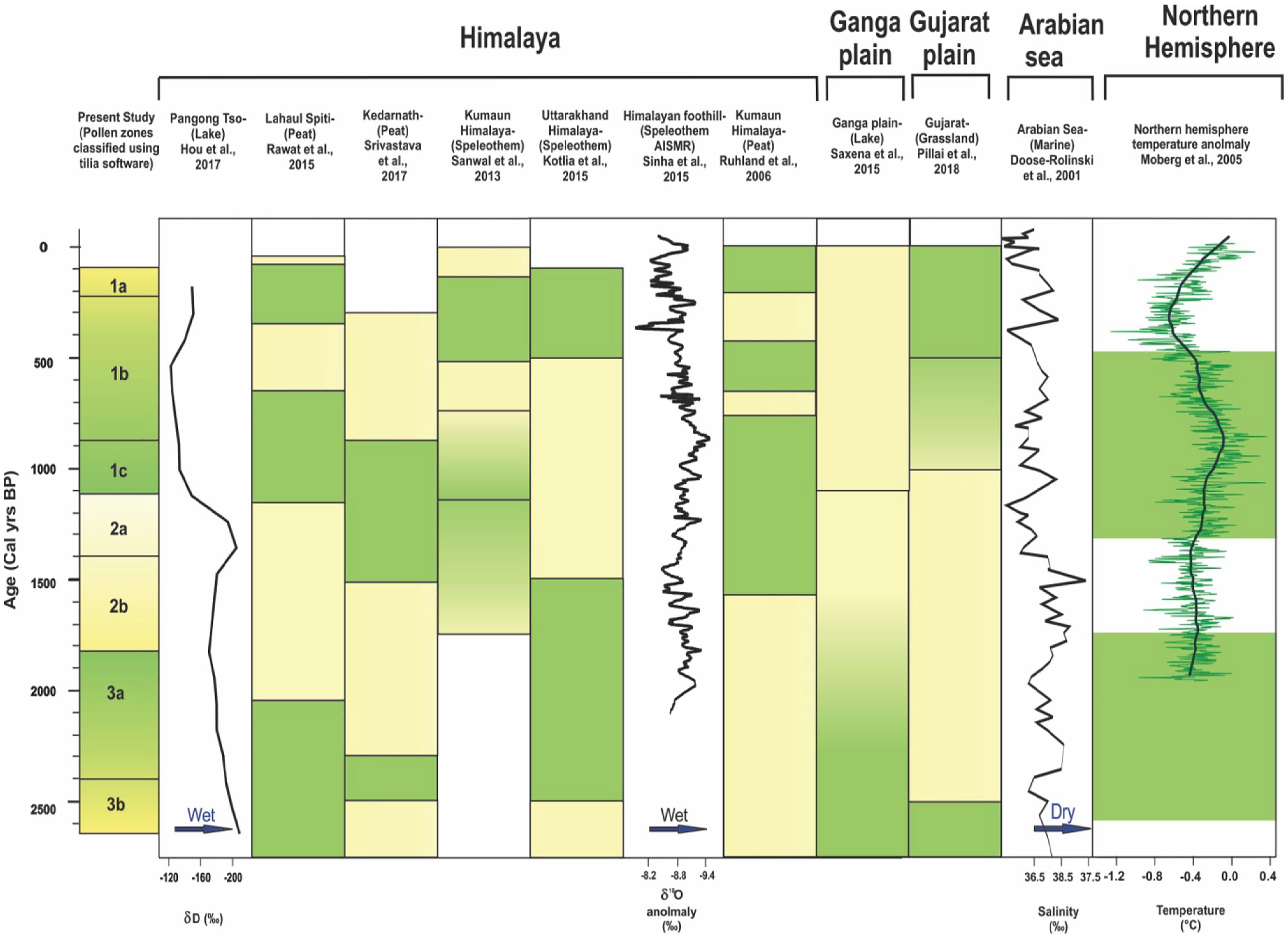
This study compared with climate records from the Himalaya, Ganga plain, Gujarat plain, Arabian Sea, and northern hemisphere temperature anomaly.

~2646 to ~1860 cal. yr BP is overall a wet phase where the basal part identified as PZ 3b spanning from ~2646 to ~2392 BP is relatively drier as shown by pollen study. This phase is characterized by increased magnetic concentration (rising χlf) and organic productivity (high TOC) and rising atmospheric nitrogen input perhaps as a result of intense biogenic activity.

δD record of compound specific leaf wax from the Pangong Tso (Ladakh) which lies in the vicinity of the study area shows gradual enrichment from ~3 ka to ~2 ka (Figure 7; Hou et al., 2017). The lower values falling within this period possibly suggest an overall strengthened ISM that is gradually decreasing (Hou et al., 2017). Furthermore, peat record from the westerly dominated Chandra Tal area, Lahaul Himalaya this phase records growth of mixed conifer broad-leaved trees, wetland and aquatic taxa (Figure 7; Rawat et al., 2015a, 2015b). Pollen and multi-proxy climate record from Kedarnath, at the northern extremity of SW Monsoon shows warm and wet climatic event from ~2.3 to 2.5 ka (Srivastava et al., 2017b). Depletion of δ¹⁸O from ~2.4 to 1.7 ka BP in NW India and speleothem record from Sainji and Sahiya cave (Central Himalaya) implies a warming trend (Kotlia et al., 2015; Sinha et al., 2015). However, our record differs from a pollen and diatom based climate record from Pinder valley (Kumaun Himalaya) (Figure 7; Rühland et al., 2006), showing an arid climate prevailing during this phase.

In the Ganga foreland, based on lake pollen record, an overall wet climate but gradual weakening of ISM is suggested by Saxena et al. (2015). Sediment geochemistry in the Rann of Kachchh, western India, also suggests a wet phase around the same time but followed by aridity (Figure 7; Pillai et al., 2018). Sediment core from the Arabian Sea suggests reduced sea surface salinity, as inferred from the oxygen isotopic content of planktonic foraminifera (Doose-Rolinski et al., 2001) implying stronger ISM.

~1860 to 1154 cal. yr BP shows prevalence of dry conditions with decline in AP, aquatic taxa and grasses (Figure 3). However, the period between ~1825 and 1400 cal. yr BP (PZ-2b) was relatively more arid where the percentage of Cyperaceae drastically reduced and climatic amelioration occurs between ~1400 and 1118 cal. yr BP (PZ-2a) when rise in aquatic pollen is witnessed. This phase as a whole shows gradually declining δ¹⁵N, lowered χlf and lighter δ¹³C_org suggesting declining atmospheric N input, lowered carbon sequestration and lowering magnetite concentration (Figure 5). It also shows an overall reduction in TC and TN (except for a brief phase of ~100 years) suggesting reduced biological activity (Figure 5a). Quantitative rise of fungal and algal spores here can be taken as a response to aridity.

δD values of Pangong Tso show enrichment during this phase suggesting a low lake level due to subdued ISM which however increases at around 1300 cal. yr BP (Figure 7; Hou et al., 2017). Pollen record from Lahaul Spiti also records arid climate from ~2 to 1.3 ka (Rawat et al., 2015a). A contemporaneous arid phase is revealed from the Kedarnath peat record and high-resolution speleothem record from Dharamjali cave (Uttarakhand) also suggests aridity in this interval (Sanwal et al., 2013; Srivastava et al., 2017b). Record from the Sainji cave, however, suggests wet climate followed by a cooling phase at around 1.5 ka (Kotlia et al., 2015). All India summer monsoon rainfall (AISMR) data from the Sahiya cave reveal reduced rainfall during ~1.5 to 1.3 ka interval. Pollen record from the Kumaun Himalaya indicates continuous aridity till ~1.6 ka after which the humidity prevailed (Rühland et al., 2006). Pollen record from Ganga and Gujarat Plains reveals progressive aridity during this timeframe (Pillai et al., 2018; Saxena et al., 2015). Contemporary to this interval, the Arabian Sea witnessed a phase of increased salinity due to reduced ISM (Doose-Rolinski et al., 2001). This hints the entire Northern India and the Western Himalaya were affected by reduced ISM during this phase (Sinha et al., 2015).

~1154 cal. yr BP to present shows an overall rise in AP and aquatics and climatic amelioration following the arid phase, although there is evidence of frequent fluctuations between wet and dry phases. Gradual fall of Chenopodiaceae/Amaranthaceae and rise in aquatic taxa emphasizes rise in moisture. This interpretation is supported by rising δ¹³C_org, δ¹⁵N, χlf, TOC, and TN within this zone possibly suggesting a warming trend (Figure 5).

δD of the Pangong Tso sediment points to gradual warming from ~500 years and suggests rising lake levels (Figure 7; Hou et al., 2017). Pollen record from the Chandra Tal, Lahaul Spiti, indicates wet phases between ~1100 and 600 ka and ~0.35 and 0.1 ka (Figure 7; Rawat et al., 2015a; Sanwal et al., 2013 also suggest alternate wet and warm phases in Kumaun Himalaya within this zone). Peat and speleothem record from Kumaun Himalaya suggests a wetter climate at ~0.5 ka (Kotlia et al., 2015; Rühland et al., 2006). Likewise, AISMR derived from speleothem in Sahiya cave (Garhwal Himalaya) suggests increasing rainfall during the last millennium to the present (Figure 7; Sinha et al., 2015). Climate of the Ganga Plains continues to be arid till present (Saxena et al., 2015). Sediment weathering and pollen records from Gujarat plain imply a warming trend from ~1 ka to present (Pillai et al., 2018). The initial phase of this zone also coincides with decreasing salinity of the Arabian Sea suggesting rise in sea level (Doose-Rolinski et al., 2001).

The record presented here broadly captures two warm phases (Zone 1 and Zone 3), which compares well with climate records derived from peat, lacustrine sediment, and speleothem from drier Ladakh, Lahaul Spiti, and wetter southern Himalayan front (Kumaun and Garhwal Himalaya). This record is also in tandem with those generated from the core monsoon zone of the Ganga Plains. These warming trends seem to follow the phases of positive temperature anomalies and stronger solar insolation in Northern Hemisphere (Figure 7; Moberg et al., 2005).

Connection with historical events and cultural changes

Climate and water availability (scarcity/excess) have been a core in influencing agriculture, human migration, and settlements of ancient civilizations of Egypt, Indian subcontinent, West Asian Region, Europe, and America (Gupta et al., 2006). Droughts and floods related to variable Asian monsoon still have devastating influence on the economy of countries (pertaining to South East Asia, the Middle East, and India) which demands thorough understanding of climate variability and human responses (Bhalme and Mooley, 1980; Singhvi and Krishnan, 2014).

This study generated a climate and vegetation record from Ladakh, the headwater of the Indus River that spans 2700 years and can be utilized to understand post Harappan civilization changes in relation to climate. The warming event (~2700 to ~1800 cal. yr BP or ~750 BC to AD ~150) shown in the bottom part of the section is broadly comparable to the Roman Warm Period (RWP) from ~550 BC to AD ~350 (2500–1600 cal. yr BP; Wang et al., 2012). This was associated with the rise of the Roman Empire and amelioration of climate making way for the growth of an agriculture-based economy (McCormick et al., 2012). During this period, as a result of increased ISM strength, agricultural production boosts bringing social and economic prosperity in India (Gupta et al., 2006). Clearing of forest with the discovery of iron engineering and spread of agriculture around Ganga plains are reported around 850 BC/2800 cal. yr BP followed by the rise of Magadha empire around 600 BC (2550 cal. yr BP) in India. Historical records also suggest the Maurya Empire practice rainwater harvesting during ~324 to 185 BC/2274 to 2135 cal. yr BP which has led to its agricultural prosperity (Pandey et al., 2003). The crossing of the Alps from France to Italy for military conquest by Hannibal (a Carthaginian general) with soldiers and animals including elephants around ~250 BC/2200 cal. yr BP would not have been possible had the Alps was covered with ice. This is a good indication of receded alpine glacier due to rise in global temperature which is also supported by various paleoclimatic data (Moffa-Sánchez and Hall, 2017; Neumann, 1992; Wang et al., 2012). This is followed by a punctuated cooling event (AD ~150 to 850/1800 to 1100 cal. yr BP) which is associated with the fall of the Western Roman Empire and is thought to have been caused by an increase in climatic variability (Büntgen et al., 2011). Reduction in agricultural harvests, political pressures, cultural metamorphosis, barbarian invasion, and migration of the central European people are reported during this period (Büntgen et al., 2011). The warming phase (AD ~850 to ~1750/1100 to 200 cal. yr BP) partly corresponds to the AD 6th to 9th socio-economic consolidation of central Europe. Reduction of climatic severity might have helped the demographic growth in the central Europe. In India, increased agricultural production, flourishing trade between Europe and Middle East, and economic growth occurred contemporaneously with these events (Gupta et al., 2006). The transition from the ‘Medieval Warm Period’ (MWP) to ‘Little Ice Age’ (LIA) also followed devastating consequences in Europe such as the Black Death Plague of AD ~14th century/0.55 ka BP and widespread famine (Büntgen et al., 2011). North western India and China also witnessed widespread drought and famine during AD 16th to 18th centuries/~3.5 to 1.5 ka BP with weaker ISM (Kotlia et al., 2012; Shen et al., 2007). Growth of population and migration are reported in India during this period (Gupta et al., 2006). Indian subcontinent, as a result of weakened ISM witnessed famines and poor agricultural productions in AD 14th to 18th centuries. To capture the best of monsoon water, mega earthworks were reported to be constructed at Deccan region during 1300–1700 BC/650–250 cal. yr BP. The Deccan plateau based Vijayanagara Empire well known for its marvelous water management technology was founded at 1614 cal. yr BP/AD 1336 (Pandey et al., 2003). The demise of the late Angkor city, Combodia in AD ~15th century/~450 cal. yr BP is placed in the transition phase from MWP to LIA. This is comparable to the rise of Cheno/Am and fall of Ranunculaceae, Caryophyllaceae, Poaceae, Cyperaceae, and aquatic taxa in the upper part of subzone PZ-1b (~943–293 cal. yr BP) of this study. Prolonged drought due to cooling is also inferred from infrastructural modifications including elaborate and large-scale water management network constructed for storage, control, and distribution of water (Fletcher et al., 2008). Such management is a sign of the struggle by the society to cope up with the scarcity of water during the onset of LIA.

These changes in relation to ancient civilizations, although coincident with climate cycles could also have occurred due to other external forces like political instabilities, diseases, and foreign invasion. Notwithstanding this, this study points out that historical events seem to be affected to a great extent by the patterns of climate cycles. There are sufficient archeological and paleoclimatic evidences in support of this statement. The present and future generations should be apprised of their vulnerability.

Conclusion

The Himalaya and the India summer monsoon are considered as lifelines for sustenance of human societies for ages. Historical and archeological evidences indicate that monsoon has driven several social and technological transformations. This study presents a 2700-year climate/monsoon variability record from a rather poorly understood Ladakh Himalayan region and concludes the following:

Climate in Ladakh Himalaya between ~2646 and 1860 cal. yr BP was relatively warm followed by a cold and dry phase between ~1860 and 1154 cal. yr BP. From ~1154 to 293 cal. yr BP climatic condition reverted to warm and wet.

The temporal correlations of climate records from across the Himalaya and its foreland (the Ganga Plain) suggest that inferred climate stratigraphy is largely uniform over north India and NW Himalaya.

The warm climatic phases appear to be overprinted onto the phases of well-documented Northern Hemisphere temperature anomaly and solar insolation and hence concurrent planetary warming may have led to a warmer and wetter phase in the high-altitude Ladakh region, and that scenario may have buttressed societal activities in the region.

Footnotes

Acknowledgements

The authors thank the Directors of Wadia Institute of Himalayan Geology, Dehradun, and Birbal Sahni Institute of Palaeosciences, Lucknow, for their support. Dr Koushik Sen is acknowledged for his help in the field. They also acknowledge Professor David Bridgland for editing the manuscript.

Funding

The author(s) received no financial support for the research, authorship, and/or publication of this article.

ORCID iD

Pradeep Srivastava

References

Agnihotri

Dutta

(2003) Centennial scale variations in monsoonal rainfall (Indian, east equatorial and Chinese monsoons): Manifestations of solar variability. Current Science 85: 459–463.

Agnihotri

Dimri

Joshi

et al. (2017) Assessing operative natural and anthropogenic forcing factors from long-term climate time series of Uttarakhand (India) in the backdrop of recurring extreme rainfall events over northwest Himalaya. Geomorphology 284: 31–40.

Agnihotri

Dutta

Soon

(2011) Temporal derivative of Total Solar Irradiance and anomalous Indian summer monsoon: An empirical evidence for a sun–climate connection. Journal of Atmospheric and Solar-Terrestrial Physics 73(13): 1980–1987.

Agnihotri

Dutta

Bhushan

et al. (2002) Evidence for solar forcing on the Indian monsoon during the last millennium. Earth and Planetary Science Letters 198(3–4): 521–527.

Bachelet

Neilson

Lenihan

et al. (2001) Climate change effects on vegetation distribution and carbon budget in the United States. Ecosystems 4(3): 164–185.

Battarbee

Thompson

Catalan

et al. (2002) Climate variability and ecosystem dynamics of remote alpine and arctic lakes: The MOLAR project. Journal of Paleolimnology 28(1): 1–6.

Bhalme

Mooley

(1980) Large-scale droughts/floods and monsoon circulation. Monthly Weather Review 108(8): 1197–1211.

Bhambri

Mehta

Singh

et al. (2017) Landslide inventory and damage assessment in the Bhagirathi Valley, Uttarakhand, during June 2013 flood. Himalayan Geology 38(2): 193–224.

Bhattacharyya

Narasimha

(2005) Possible association between Indian monsoon rainfall and solar activity. Geophysical Research Letters 32(5): L05813.

10.

Bookhagen

Burbank

(2010) Toward a complete Himalayan hydrological budget: Spatiotemporal distribution of snowmelt and rainfall and their impact on river discharge. Journal of Geophysical Research: Earth Surface 115: F03019.

11.

Brookfield

Reynolds

(1981) Late Cretaceous emplacement of the Indus suture zone ophiolitic melanges and an Eocene-Oligocene magmatic arc on the northern edge of the Indian plate. Earth and Planetary Science Letters 55(1): 157–162.

12.

Buggle

Hambach

Müller

et al. (2014) Iron mineralogical proxies and quaternary climate change in SE-European loess–paleosol sequences. CATENA 117: 4–22.

13.

Büntgen

Tegel

Nicolussi

et al. (2011) 2500 years of European climate variability and human susceptibility. Science 331(6017): 578–582.

14.

Chevuturi

Dimri

Thayyen

(2018) Climate change over Leh (Ladakh), India. Theoretical and Applied Climatology 131(1–2): 531–545.

15.

Demske

Tarasov

Leipe

et al. (2016) Record of vegetation, climate change, human impact and retting of hemp in Garhwal Himalaya (India) during the past 4600 years. The Holocene 26(10): 1661–1675.

16.

Demske

Tarasov

Wünnemann

et al. (2009) Late glacial and Holocene vegetation, Indian monsoon and westerly circulation in the Trans-Himalaya recorded in the lacustrine pollen sequence from Tso Kar, Ladakh, NW India. Palaeogeography, Palaeoclimatology, Palaeoecology 279(3): 172–185.

17.

Dimri

Thayyen

Kibler

et al. (2016) A review of atmospheric and land surface processes with emphasis on flood generation in the Southern Himalayan rivers. Science of the Total Environment 556: 98–115.

18.

Dixit

Tandon

(2016) Hydroclimatic variability on the Indian subcontinent in the past millennium: Review and assessment. Earth-Science Reviews 161: 1–15.

19.

Dixit

Hodell

Petrie

(2014) Abrupt weakening of the summer monsoon in northwest India ~4100 yr ago. Geology 42(4): 339–342.

20.

Dixit

Hodell

Giesche

et al. (2018) Intensified summer monsoon and the urbanization of Indus Civilization in northwest India. Scientific Reports 8(1): 4225.

21.

Dobhal

Mehta

Srivastava

(2013) Influence of debris cover on terminus retreat and mass changes of Chorabari Glacier, Garhwal region, central Himalaya, India. Journal of Glaciology 59(217): 961–971.

22.

Doose-Rolinski

Rogalla

Scheeder

(2001) High-resolution temperature and evaporation changes during the late-Holocene in the northeastern Arabian Sea. Paleoceanography and Paleoclimatology 16(4): 358–367.

23.

Durani

Singh

Kachroo

(1975) Phytosociological Studies on the Vegetation of Ladakh Desert (India). Jodhpur, India: Annals of Arid Zone.

24.

Dutt

Gupta

Wünnemann

et al. (2018) A long arid interlude in the Indian summer monsoon during ~4,350 to 3,450 cal. yr BP contemporaneous to displacement of the Indus valley civilization. Quaternary International 482: 83–92.

25.

Egli

Lowrie

(2002) Anhystereticremanent magnetization of fine magnetic particles. Journal of Geophysical Research: Solid Earth 107(B10): 2209.

26.

Eisner

Peterson

(1998) Pollen, fungi and algae as age indicators of drained lake basins near Barrow, Alaska. In: 7th international conference on permafrost (Collection Nordicana, 57), Yellowknife, NWT, Canada, 23–27 June 1998, pp. 245–250. Laval, QC, Canada: Centre de etudes nordiques de l’Universite Laval.

27.

Erdtman

(1943) An Introduction to Pollen Analysis (ChronicaBotanica, New series of plant science books), vol. 12. Waltham, MA: Chronica Botanica Company.

28.

Eyre

(1997) Frequency dependence of magnetic susceptibility for populations of single-domain grains. Geophysical Journal International 129(1): 209–211.

29.

Fletcher

Pottier

Evans

(2008) The development of the water management system of Angkor: A provisional model. Bulletin of the Indo-Pacific Prehistory Association 28: 57–66.

30.

Gadgil

Vinayachandran

Francis

et al. (2004) Extremes of the Indian summer monsoon rainfall, ENSO and equatorial Indian Ocean oscillation. Geophysical Research Letters 31(12): L12213.

31.

Grimm

(1987) CONISS: A FORTRAN 77 program for stratigraphically constrained cluster analysis by the method of incremental sum of squares. Computers & Geosciences 13(1): 13–35.

32.

Grimm

(1993) TILIA: A Pollen Program for Analysis and Display. Springfield, IL: Illinois State Museum.

33.

Gupta

(2004) Origin of agriculture and domestication of plants and animals linked to early Holocene climate amelioration. Current Science 87: 54–59.

34.

Gupta

Anderson

Pandey

et al. (2006) Adaptation and human migration, and evidence of agriculture coincident with changes in the Indian summer monsoon during the Holocene. Current Science 90(8): 1082–1090.

35.

Gupta

Das

Anderson

(2005) Solar influence on the Indian summer monsoon during the Holocene. Geophysical Research Letters 32(17): L17703.

36.

Gupta

Mohan

Das

et al. (2013) Solar forcing of the Indian summer monsoon variability during the Ållerød period. Scientific Reports 3: 2753.

37.

Gupta

Sharma

(1986) Pollen flora of north-west Himalaya. Lucknow, India: Indian Association of Palynostratigraphers.

38.

Henderson

Najman

Parrish

et al. (2011) Constraints to the timing of India–Eurasia collision; a re-evaluation of evidence from the Indus Basin sedimentary rocks of the Indus–Tsangpo Suture Zone, Ladakh, India. Earth-Science Reviews 106(3–4): 265–292.

39.

Hewitt

(1998a) Catastrophic landslides and their effects on the Upper Indus streams, Karakoram Himalaya, northern Pakistan. Geomorphology 26(1–3): 47–80.

40.

Hewitt

(1998b) Glaciers receive a surge of attention in the Karakoram Himalaya. Eos, Transactions American Geophysical Union 79(8): 104–105.

41.

Hobley

Sinclair

Mudd

(2012) Reconstruction of a major storm event from its geomorphic signature: The Ladakh floods, 6 August 2010. Geology 40(6): 483–486.

42.

Honegger

Dietrich

Frank

et al. (1982) Magmatism and metamorphism in the Ladakh Himalayas (the Indus-Tsangpo suture zone). Earth and Planetary Science Letters 60(2): 253–292.

43.

Hou

D’Andrea

Wang

et al. (2017) Influence of the Indian monsoon and the subtropical jet on climate change on the Tibetan Plateau since the late Pleistocene. Quaternary Science Reviews 163: 84–94.

44.

Jain

(2014) When did India–Asia collide and make the Himalaya? Current Science 106: 254–266.

45.

Kala

(2011) Floral diversity and distribution in the high altitude cold desert of Ladakh, India. Journal of Sustainable Forestry 30(5): 360–369.

46.

Karim

Veizer

(2002) Water balance of the Indus River Basin and moisture source in the Karakoram and western Himalayas: Implications from hydrogen and oxygen isotopes in river water. Journal of Geophysical Research 107(D18): ACH 9-1–ACH 9-12.

47.

Kathayat

Cheng

Sinha

et al. (2017) The Indian monsoon variability and civilization changes in the Indian subcontinent. Science Advances 3(12): e1701296.

48.

Kotlia

Ahmad

Zhao

J-X

et al. (2012) Climatic fluctuations during the LIA and post-LIA in the Kumaun Lesser Himalaya, India: Evidence from a 400 y old stalagmite record. Quaternary International 263: 129–138.

49.

Kotlia

Singh

Joshi

et al. (2015) Precipitation variability in the Indian Central Himalaya during last ca. 4,000 years inferred from a speleothem record: Impact of Indian Summer Monsoon (ISM) and Westerlies. Quaternary International 371: 244–253.

50.

Kumar

Srivastava

Meena

(2017) Late Pleistocene aeolian activity in the cold desert of Ladakh: A record from sand ramps. Quaternary International 443: 13–28.

51.

Lang

Barros

(2004) Winter storms in the central Himalayas. Journal of the Meteorological Society of Japan 82(3): 829–844.

52.

Leipe

Demske

Tarasov

et al. (2014) Potential of pollen and non-pollen palynomorph records from Tso Moriri (Trans-Himalaya, NW India) for reconstructing Holocene limnology and human–environmental interactions. Quaternary International 348: 113–129.

53.

Liu

Banerjee

Jackson

et al. (2004) Grain sizes of susceptibility and anhystereticremanent magnetization carriers in Chinese loess/paleosol sequences. Journal of Geophysical Research: Solid Earth 109(B3): B03101.

54.

Liu

Torrent

et al. (2010) Environmental magnetic study of a Xeralfchronosequence in northwestern Spain: Indications for pedogenesis. Palaeogeography, Palaeoclimatology, Palaeoecology 293(1–2): 144–156.

55.

Liu

Roberts

Larrasoana

et al. (2012) Environmental magnetism: Principles and applications. Reviews of Geophysics 50(4): RG4002.

56.

Wen

et al. (2010) Millennial-centennial scales climate changes of Holocene indicated by magnetic susceptibility of high-resolution section in Salawusu River valley, China. Chinese Geographical Science 20(3): 243–251.

57.

McCormick

Büntgen

Cane

et al. (2012) Climate change during and after the Roman Empire: Reconstructing the past from scientific and historical evidence. Journal of Interdisciplinary History 43(2): 169–220.

58.

Moberg

Sonechkin

Holmgren

et al. (2005) Highly variable Northern Hemisphere temperatures reconstructed from low- and high-resolution proxy data. Nature 433(7026): 613–617.

59.

Moffa-Sánchez

Hall

(2017) North Atlantic variability and its links to European climate over the last 3000 years. Nature Communications 8(1): 1726.

60.

Moore

Webb

(1978) Illustrated Guide to Pollen Analysis. London: Hodder & Stoughton.

61.

Moore

Webb

Collison

(1991) Pollen Analysis. London: Blackwell Scientific Publications.

62.

Neumann

(1992) Climatic conditions in the Alps in the years about the year of Hannibal’s crossing (218 BC). Climatic Change 22(2): 139–150.

63.

Pandey

Gupta

Anderson

(2003) Rainwater harvesting as an adaptation to climate change. Current Science 85(1): 46–59.

64.

Pillai

Anoop

Prasad

et al. (2018) Multi-proxy evidence for an arid shift in the climate and vegetation of the Banni grasslands of western India during the mid- to late-Holocene. The Holocene 28(7): 1057–1070.

65.

Pokharia

Agnihotri

Sharma

et al. (2017) Altered cropping pattern and cultural continuation with declined prosperity following abrupt and extreme arid event at ~4,200 yrs BP: Evidence from an Indus archaeological site Khirsara, Gujarat, western India. PLoS ONE 12(10): e0185684.

66.

Prasad

Anoop

Riedel

et al. (2014) Prolonged monsoon droughts and links to Indo-Pacific warm pool: A Holocene record from Lonar Lake, central India. Earth and Planetary Science Letters 391: 171–182.

67.

Punt

Hoen

Blackmore

et al. (2007) Glossary of pollen and spore terminology. Review of Palaeobotany and Palynology 143(1–2): 1–81.

68.

Quamar

Ali

Pandita

et al. (2018) Modern pollen assemblages from Reasi (Jammu and Kashmir), India: A tool for interpreting fossil pollen records. Grana 57(5): 364–376.

69.

Rana

Sundriyal

Juyal

(2012) Recent cloudburst-induced landslides around Okhimath, Uttarakhand. Current Science 103(12): 1389–1390.

70.

Rawat

Gupta

Sangode

et al. (2015a) Late Pleistocene–Holocene vegetation and Indian summer monsoon record from the Lahaul, northwest Himalaya, India. Quaternary Science Reviews 114: 167–181.

71.

Rawat

Gupta

Srivastava

et al. (2015b) A 13,000 year record of environmental magnetic variations in the lake and peat deposits from the Chandra valley, Lahaul: Implications to Holocene monsoonal variability in the NW Himalaya. Palaeogeography, Palaeoclimatology, Palaeoecology 440: 116–127.

72.

Reimer

Bard

Bayliss

et al. (2013) IntCal13 and Marine13 radiocarbon age calibration curves 0–50,000 years cal BP. Radiocarbon 55(4): 1869–1887.

73.

Roxy

Ritika

Terray

et al. (2015) Drying of Indian subcontinent by rapid Indian Ocean warming and a weakening land-sea thermal gradient. Nature Communications 6: 7423.

74.

Rühland

Phadtare

Pant

et al. (2006) Accelerated melting of Himalayan snow and ice triggers pronounced changes in a valley peatland from northern India. Geophysical Research Letters 33(15): L15709.

75.

Sagwal

(1991) Ladakh, Ecology and Environment. Ladakh, India: APH Publishing.

76.

Sangode

Meshram

Rawat

et al. (2017) Sedimentary and geomorphic signatures of a cloud burst and triggered flash floods in the Indus valley of Ladakh Himalaya. Himalayan Geology 38(1): 12–29.

77.

Sanwal

Kotlia

Rajendran

et al. (2013) Climatic variability in Central Indian Himalaya during the last ~1800 years: Evidence from a high resolution speleothem record. Quaternary International 304: 183–192.

78.

Saxena

Trivedi

Chauhan

et al. (2015) Holocene vegetation and climate change in Central Ganga Plain: A study based on multiproxy records from Chaudhary-Ka-Tal, Raebareli District, Uttar Pradesh, India. Quaternary International 371: 164–174.

79.

Sharma

Shukla

Bartarya

et al. (2017) The Holocene floods and their affinity to climatic variability in the western Himalaya, India. Geomorphology 290: 317–334.

80.

Shen

Wang

Hao

et al. (2007) Exceptional drought events over eastern China during the last five centuries. Climatic Change 85(3–4): 453–471.

81.

Singhvi

Krishnan

(2014) Past and the present climate of India. In: Kale

(ed.) Landscapes and Landforms of India. Dordrecht: Springer, pp. 15–23.

82.

Sinha

Kathayat

Cheng

et al. (2015) Trends and oscillations in the Indian summer monsoon rainfall over the last two millennia. Nature Communications 6: 7309.

83.

Srivastava

Agnihotri

Sharma

et al. (2017a) 8000-year monsoonal record from Himalaya revealing reinforcement of tropical and global climate systems since mid-Holocene. Scientific Reports 7(1): 14515.

84.

Srivastava

Kumar

Chaudhary

et al. (2017b) Paleofloods records in Himalaya. Geomorphology 28: 17–30.

85.

Srivastava

Kumar

Mishra

et al. (2013) Early Holocene monsoonal fluctuations in the Garhwal higher Himalaya as inferred from multi-proxy data from the Malari paleolake. Quaternary Research 80(3): 447–458.

86.

Stockmarr

(1971) Tablets with spores used in absolute pollen analysis. Pollen Spores 13: 615–621.

87.

Stuiver

Reimer

Bard

et al. (1998) INTCAL98 radiocarbon age calibration, 24,000–0 cal BP. Radiocarbon 40(3): 1041–1083.

88.

Sundriyal

Shukla

Rana

et al. (2015) Terrain response to the extreme rainfall event of June 2013: Evidence from the Alaknanda and Mandakini River Valleys, Garhwal Himalaya, India. Episodes 38(3): 179–188.

89.

Van Campo

Cour

Sixuan

(1996) Holocene environmental changes in Bangong Co basin (Western Tibet). Part 2: The pollen record. Palaeogeography, Palaeoclimatology, Palaeoecology 120(1–2): 49–63.

90.

Van Geel

(1986) Application of fungal and algal remains and other microfossils in palynological analyses. In: Berglund

(ed.) Handbook of Holocene Palaeoecology and Palaeohydrology. Chichester: Wiley, pp. 497–505.

91.

Wang

Surge

Mithen

(2012) Seasonal temperature variability of the Neoglacial (3300–2500 BP) and Roman warm period (2500–1600 BP) reconstructed from oxygen isotope ratios of limpet shells (Patella vulgata), Northwest Scotland. Palaeogeography, Palaeoclimatology, Palaeoecology 317: 104–113.

92.

Wasson

Sundriyal

Chaudhary

et al. (2013) A 1000-year history of large floods in the Upper Ganga catchment, central Himalaya, India. Quaternary Science Reviews 77: 156–166.

93.

Webster

Toma

Kim

(2011) Were the 2010 Pakistan floods predictable? Geophysical Research Letters 38(4): L04806.

94.

Wünnemann

Demske

Tarasov

et al. (2010) Hydrological evolution during the last 15 kyr in the Tso Kar lake basin (Ladakh, India), derived from geomorphological, sedimentological and palynological records. Quaternary Science Reviews 29(9–10): 1138–1155.

95.

Yadav

Gupta

Kotlia

et al. (2017) Recent wetting and glacier expansion in the northwest Himalaya and Karakoram. Scientific Reports 7(1): 6139.

96.

Zhong

Wei

Chen

et al. (2017) A 15.4-ka paleoclimate record inferred from δ¹³C and δ¹⁵N of organic matter in sediments from the sub-alpine Daping Swamp, western Nanling Mountains, South China. Journal of Paleolimnology 57(2): 127–139.

97.

Ziegler

Cantarero

Wasson

et al. (2016) A clear and present danger: Ladakh’s increasing vulnerability to flash floods and debris flows. Hydrological Processes 30(22): 4214–4223.

98.

Ziegler

Wasson

Bhardwaj

et al. (2014) Pilgrims, progress, and the political economy of disaster preparedness – The example of the 2013 Uttarakhand flood and Kedarnath disaster. Hydrological Processes 28(24): 5985–5990.

High-resolution climatic (monsoonal) variability reconstructed from a continuous ~2700-year sediment record from Northwest Himalaya (Ladakh)

Abstract

Keywords

Introduction

Study site and regional setting

Geology

Climate of the region

Modern vegetation in the region

Methodology

Sampling, chronology, and age-depth model

Pollen analysis

Environmental magnetism

TOC, TN, and stable isotopic composition (δ13C, δ15N)

Results

Lithosection, adopted chronological model and temporal resolution

Palynology

PZ-3 (~2646 to 1860 cal. yr BP; 123–79 cm)

PZ-2 (~1860 to 1154 cal. yr BP; 79–39 cm)

PZ-1 (1154 cal. yr BP to present; 39–0 cm)

Sedimentary TOC, TN contents, and stable isotopes (δ13C, δ15N)

Environmental magnetism

Proxy response to climate (monsoonal) change

Climatic history, regional correlations, and forcing factors

Connection with historical events and cultural changes

Conclusion

Footnotes

Acknowledgements

Funding

ORCID iD

References

TOC, TN, and stable isotopic composition (δ¹³C, δ¹⁵N)

Sedimentary TOC, TN contents, and stable isotopes (δ¹³C, δ¹⁵N)