Late-Holocene: Cooler or warmer?

Abstract

Early studies on the evolution of glaciers argue that the warm Early Holocene transitioned into a Late-Holocene Neoglacial, with numerous glacial advances due to decreasing solar forcing in the boreal summer. The assumption of decreasing temperatures based on the glacier studies was supported by several proxy-based reconstructions as well as by simulations. Under the keyword “Holocene temperature conundrum” this fact is questioned. In particular, it is argued that the proxy studies are biased on time series dominated by a seasonal bias in the form of predominant summer temperatures (mainly marine). After a presentation of the facts, the weaknesses of both hypotheses (cooler or warmer) are briefly presented.

Keywords

glacier growth Holocene neoglacial orbital forcing proxy studies recent publications temperature conundrum

The present interglacial, called the Holocene, started about 11,700 cal years before present (BP) and is often subdivided into three periods (Walker et al., 2012; Wanner et al., 2011). In recent literature, the third period is usually called Neoglacial or Neoglaciation, because most glaciers started growing after their considerable retreats during the Holocene Thermal Maximum (Wanner et al., 2008), also known as the Holocene Climatic Optimum, Altithermal, Hypsithermal or Megathermal (Deevey and Flint, 1957). During this warm period, between about 10,000 and 5500 years BP, proxy-based reconstructions and selected simulations show that the mean annual temperature was about 2–3°C higher than today and differed from region to region (Fischer et al., 2018; Kaufman et al., 2004; Renssen et al., 2012).

Increasingly growing glaciers

The term Neoglaciation was probably first used by Porter and Denton (1967), who reconstructed several multi-century glacier advances and retreats in the North American Cordillera. In their seminal study, Denton and Karlén (1973) concluded that the Holocene experienced alternating intervals of glacier advances lasting 600–900 years, and retreats lasting up to 1750 years. Figure 1 shows the detected frequency of advances of large glaciers during the Holocene, separated for three regions of the globe (Solomina et al., 2015).

Figure 1.

Vertical bars: Number of advances by larger glaciers during the Holocene, divided into three regions of the globe (Solomina et al., 2015). The magenta line shows the solar insolation during boreal summer (June) for 60°N. The red arrow marks the time of the death of Ötzi.

A greater number of early advances occurred prior to 11,000 BP and around 8200 BP, predominantly in the Northern Hemisphere. These early advances were mainly the result of cold snaps due to freshwater outbursts from the proglacial lakes Agassiz and Ojibway in North America which induced a downturn of the North Atlantic thermohaline circulation (Kleiven et al., 2008; Matero et al., 2017; Rohling and Pälike, 2005). After the middle of the sixth millennium BP there was an obvious increase in the number of glacier advances worldwide. The increasing frequency culminated during the cold relapses of the Little Ice Age between the mid-14th and the mid-19th centuries (Figure 1). This late-Holocene cooling started earlier in the Northern Hemisphere (Neukom et al., 2014), where its signal was stronger. It was clearly detected in temperature reconstructions based on the analysis of Greenland ice cores (Fisher and Koerner, 2002).

It is evident that the glacier mass balance is a suitable proxy, mainly for summer temperature, but solid winter precipitation also contributes, although to a lesser extent (Oerlemans and Reichert, 2000; Reichert et al., 2001; Steiner et al., 2005). Based on the first-order theory of glacier dynamics, Oerlemans (2005) constructed a global temperature signal based on 169 glacier length records, which documents the cooling of the Little Ice Age after AD 1600.

Key role of orbital forcing

Very often the increasing frequency of glacier advances is associated with decreasing boreal summer insolation at the higher northern midlatitudes (see the magenta curve in Figure 1). Solar insolation is also considered a key parameter in explaining the initiation of ice ages, supported by Arctic amplification, namely through the growing Arctic sea ice and a longer-lasting snow cover over the northern continental areas (Bassinot et al., 1994). Above all, the long-lasting cool period of the Neoglacial is impressively symbolized by the mummy of the iceman Ötzi, who died about 5250 years BP in a rocky gully at an altitude of 3210 m above sea level, close to the Tisenjoch pass in the southern Austrian Alps (Fleckinger, 2018; Maixner et al., 2016). Ötzi was preserved in the ice, and his body was only revealed after the positive temperature jump in the late 1980s (IPCC, 2013: 14, Figure 2). Figure 2 shows Ötzi’s body and how it was found by German hikers Erika and Helmut Simon on September 21, 1991 (Fleckinger, 2018).

Figure 2.

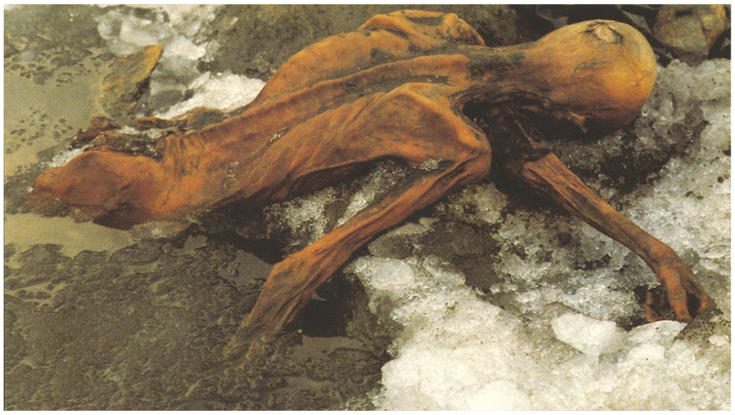
Photo of how the Similaun Man “Ötzi” was found by Erika and Helmut Simon on September 21, 1991.

Together with the influence of the melting ice sheets, orbital forcing was likely the key factor that triggered late-Holocene cooling, mainly during boreal summer. Figure 3 presents the latitudinal insolation anomalies of the Holocene for austral summer (December), boreal summer (June), and for the annual mean, relative to present (after Marcott et al., 2013). The annual mean insolation (Figure 3c) is significantly influenced by the axial tilt (obliquity). It therefore exhibits a symmetrical spatial pattern with higher insolation in the early Holocene at both poles. The two seasonal patterns in Figure 3a and b rather indicate an asymmetry that is mainly the result of the 23,000-year-long precession cycle (Huybers, 2007). The maximum rate of change with strongly decreasing (increasing) summer insolation rates in the Northern (Southern) Hemisphere occurred in the period from 8000 to 4000 years BP. The strong climatic shift in the later phase of this period is often referred to as the Holocene Climate Transition (Steig, 1999; Wanner et al., 2008).

Figure 3.

Holocene climate: (a) Anomalies of surface solar insolation for austral summer (December; W/m²). (b) Same as (a), but for boreal summer (June). (c) Same as (a), but for annual mean (from: Wanner, 2016; after Berger and Loutre, 1991 and Marcott et al., 2013).

There is no doubt that other factors, including internal variability, contributed to the late-Holocene cooling. In particular, the circulation processes in the world’s large oceans must have played an important role (Orme et al., 2020; Rosenthal et al., 2013; Stott et al., 2004; Yan and Liu, 2019). In addition, it can be questioned whether the summer warming of the northern oceans was transferred to the Southern Hemisphere via the deep ocean circulation system. A lively debate also revolves around the question of whether or not greenhouse gases (GHGs) already had a decisive influence on the climate of the early to mid-Holocene (Joos et al., 2004; Ruddiman, 2016). In addition, the role of dust and aerosols must be taken into account (Liu et al., 2018).

The Holocene temperature conundrum

The decreasing solar insolation during the boreal summer led to a reduced meridional temperature gradient between the cooler ocean and the continental area and, therefore, to a southern shift of the Intertropical Convergence Zone (ITCZ). This shift resulted in a weakening of the African and Asian summer monsoon systems and, consequently, caused strong dryness with desertification processes and dust production (Haug, 2001; Wanner et al., 2008). In their simulation, Yan and Liu (2019) show that this event, which culminated around 4200 years BP, was characterized by a cooler Northern and a warmer Southern Hemisphere. They suspect this event was mainly caused by internal variability. It also caused significant cultural changes, namely the Neolithic–Bronze Age transition. The retreating summer monsoon areas in the Northern Hemisphere (African Sahel zone, Egypt, Mesopotamia, India, and China) were most severely affected. Therefore, the exploration of social and political transformation processes in these areas is an important field of activity for archaeologists (Manning and Timpson, 2014; Weiss et al., 1993). The Holocene Climate Transition of the fifth millennium BP denotes a clear shift and reorganization of the atmospheric and oceanic circulation system. Therefore, it can even be argued that the climatic character of the Holocene was quasi-bimodal (Wanner and Brönnimann, 2012). Beside the spatial redistribution of humidity, triggered by the weakening Northern Hemisphere monsoon systems, remarkable temperature changes occurred. The predominant question is whether the late-Holocene was cooler or warmer than its earlier counterpart. The discussion around this question exists under the keyword “Holocene temperature conundrum.” It was provoked by earlier reviews (Mayewski et al., 2004; Wanner et al., 2008), but especially by the study of Marcott et al. (2013), who reconstructed regional and global surface temperatures for the past 11,300 years, based on globally distributed records, most of which originated from marine records.

Figure 4a, which is based on the reconstruction by Marcott et al. (2013), shows a warming of 0.6°C culminating around 7000 years BP. It was followed by a continuing cooling. This temperature pattern was confirmed earlier by other proxy reconstructions (Kaufman et al., 2004; Ljungqvist, 2011) as well as by model studies (Renssen et al., 2009, 2012), which mostly demonstrate that the influence of orbital forcing, together with the melting ice sheets in North America and Eurasia, played a major role.

Figure 4.

Selection of Holocene temperature curves, partly supplemented by their corresponding uncertainty bars. (a) Multi-proxy-based reconstruction of global mean surface temperature after Marcott et al. (2013; reference period: 1961–1990). (b) Simulation of global mean surface temperature (after Liu et al., 2014). (c) Pollen based reconstruction of annual mean temperature for North America and Europe after Marsicek et al. (2018; reference period 1450–1950 AD). (d) Multi-proxy-based reconstruction of global mean surface temperature after Kaufman et al. (2020b; reference period 1900–2000). (e) Normalized time series (standard deviation units) of annual and summer temperature for the Southern Hemisphere (after Kaufman et al., 2020a). (f) Non-corrected (blue) and corrected (red) curves of annual mean sea surface temperature anomalies after Bova et al. (2021).

These facts were first scrutinized in the paper of Liu et al. (2014), who argued that transient simulations show late-Holocene warming mainly triggered by retreating ice sheets and rising atmospheric GHGs. Figure 4b shows their result in the form of the global mean temperature of three simulations that include orbitally driven insolation, GHGs, continental ice sheets, and their associated meltwater fluxes. The simulations show a progressive warming until about 4000 years BP, followed by more stable conditions. The comparison with reconstructed temperatures shows that these were about 1°C warmer in the early Holocene and that they converge with the simulated temperatures in the late-Holocene.

The warming argument was further supported by Liu et al. (2018), who demonstrated that reduced atmospheric dust loading generates warming, and by several proxy-based reconstructions, namely Marsicek et al. (2018). Based on the analysis of subfossil pollen from 642 sites across North America and Europe, they show that their reconstruction nicely matches the simulations as shown in Figure 4b, and that the cooling was limited to the North Atlantic records (Figure 4c). Baker et al. (2017) analyzed two stalagmites from Kinderlinskaja Cave in the southern Ural Mountains. They document a warming tendency during the winter season from 11,700 years ago until the present, and conclude that winter climate dynamics dominate the Holocene temperature evolution in the continental interior of Eurasia.

Revival of the conundrum discussion

The discussion about the Holocene conundrum was reignited by a series of new papers which again consider both variants of the conundrum as possible. The proxy-based papers of Kaufman et al. (2020a, 2020b) indicate the existence of late-Holocene cooling. Figure 4d shows the reconstruction by Kaufman et al. (2020b) that is based on the time series from 679 sites covering at least 4000 years. The warmest interval took place around 6500 years BP when GMST was 0.7°C warmer than the 19th century. In addition to this global overview in Figure 4d, Kaufman et al. (2020a) also present composites of normalized time series showing regional and seasonal differences. In the Northern Hemisphere (not shown) the differences between winter and summer are minimal and the curve resembles those in Figure 4d. The temperature peak appeared around 7000 years BP, which coincides with the high early Holocene solar insolation maximum in summer (Figure 2b). A special feature is visible in the Southern Hemisphere (Figure 4e). The annual mean shows a continuous cooling between 10,000 and 3000 years BP, followed by a subsequent warming of about 0.6°C. Only the summer season is represented. It shows a strong early Holocene warming, culminating around 5200 years BP, and a late-Holocene cooling, which is rather surprising when considering the solar insolation in Figure 3a.

Publications which include simulation results almost exclusively support the warming hypothesis. Simulations in the framework of the PMIP4-CMIP6 program, which compares the mean annual temperatures of the mid-Holocene with the preindustrial period, show that mean annual temperature increased in the high northern and southern latitudes and over Europe, but decreased elsewhere (Brierley et al., 2020). Bader et al. (2020) performed a transient Holocene simulation from 8000 BP until 1850 CE, which includes orbital, volcanic, solar irradiance, GHG and ozone forcing as well as land-use changes. They show that a global warming and a cooling mode, which probably coexisted during the Holocene, can be statistically distinguished. The warming mode is most pronounced in the tropics and dominates the mid-Holocene, whereas the cooling mode is more of a phenomenon in the Northern Hemisphere and predominates during the late-Holocene. Is it conceivable that the cooling mode mirrors periods that, during a Grand Solar Minimum, also had several large volcanic eruptions, as was typically the case during the Dark Ages (Büntgen et al., 2016) or the Little Ice Age (Bradley et al., 2016). In the most recent paper, Bova et al. (2021) present an analysis from marine sediment cores covering the last and present interglacial. They argue that the SST domination of the data set analyses reflects seasonal rather than annual temperatures, and that the Holocene Thermal Maximum was driven by boreal summer insolation (Figure 3b). The sensitivity of the SSTs to seasonal insolation during the last and warmer interglacial was used as a benchmark to remove the seasonal (mostly summer) bias. The study is valid for the area between 40°N and 40°S. The non-corrected blue curve on Figure 4f shows a peak between 10,000 and 6000 years BP. The red curve with the correction of the seasonal bias matches quite well with the simulations represented in Figure 4b.

Cooler or warmer?

What is the right answer? A final statement is not yet possible. What are the weak arguments in studies that indicate cooling? First, most studies are mainly based on marine archives which are in many cases biased by seasonal (summer) temperatures. Second, the boreal winter season, representing a strongly increasing solar insolation in the tropical area and the area of the Southern Hemisphere (Figure 2a), is only weakly represented by proxies. Third, even selected proxy studies also indicate warming (Baker et al., 2017; Marsicek et al., 2018).

What are the weaknesses of the warming argument? First, selected papers based on simulations support the cooling hypothesis (Crucifix et al., 2002; Renssen et al., 2006). Second, important forcings, partly indicating gradual warming (e.g. solar, land use, and dust), were not included in all simulations. Third, most studies (e.g. Bova et al., 2021) do not include the very high latitudes and, therefore, the important contribution of polar amplification.

What needs to be done? Transient simulations must include solar irradiance forcing as well as land-use changes (e.g. vegetation feedback) and the important influence of dust. They also must include stratospheric chemistry and dynamics and be able to correctly reproduce meltwater fluxes, meridional overturning circulation (MOC), and the most important longer-term climate modes, such as PDO and AMO. Data studies must guarantee sufficient spatial and temporal density and include as much data as possible from the Southern Hemisphere and both polar regions. They also must strive for a balanced distribution of marine and continental data, including summer and winter seasons. In any case, global annual mean temperatures are the result of a complex pattern representing a high spatial and temporal variability which is actually not represented in many studies.

Footnotes

Acknowledgements

I would like to thank Tamara Baumann for processing the figures, Angela Wade for proofreading the English text, and Olga Solomina for providing Figure 1. I also warmly thank the late Gerlinde Haid who provided the photo in . Sincere thanks also go to Oliver Timm for his support concerning model data and to the two anonymous reviewers who helped to clarify the arguments.

Funding

The author(s) received no financial support for the research, authorship, and/or publication of this article.

ORCID iD

H Wanner

References

Bader

Jungclaus

Krivova

, et al. (2020) Global temperature modes shed light on the Holocene temperature conundrum. Nature Communications 11(1): 1–8.

Baker

Lachniet

Chervyatsova

, et al. (2017) Holocene warming in western continental Eurasia driven by glacial retreat and greenhouse forcing. Nature Geoscience 10: 430–436.

Bassinot

Labeyrie

Vincent

, et al. (1994) The astronomical theory of climate and the age of the Brunhes-Matuyama magnetic reversal. Earth and Planetary Science Letters 126: 91–108.

Berger

Loutre

M-F

(1991) Insolation values for the climate of the last 10 million years. Quaternary Science Reviews 10: 297–317.

Bova

Rosenthal

Liu

, et al. (2021) Seasonal origin for the Holocene and last interglacial thermal maximum. Nature 589: 548–553.

Bradley

Wanner

Diaz

(2016) The medieval quiet period. The Holocene 26(6): 990–993.

Brierley

Zhao

Harrison

, et al. (2020) Large-scale features and evaluation of the PMIP4-CMIP6 mid-Holocene simulations. Climate of the Past 16: 1847–1872.

Büntgen

Myglan

Ljungqvist

(2016) Cooling and societal change during the Late Antique Little Ice Age from 536 to around 660 AD. Nature Geoscience 9(3): 231–236.

Crucifix

Loutre

M-F

Tulkens

, et al. (2002) Climate evolution during the Holocene: A study with an Earth system model of intermediate complexity. Climate Dynamics 19: 43–60.

10.

Deevey

Flint

(1957) Postglacial hypsithermal interval. Science 125: 182–185.

11.

Denton

Karlén

(1973) Holocene climatic variations – their pattern and possible cause. Quaternary Research 3: 155–205.

12.

Fischer

Meissner

Mix

, et al. (2018) Paleoclimate constraints on the impact of 2°C anthropogenic warming and beyond. Nature Geoscience 11: 474–485.

13.

Fisher

Koerner

(2002) Holocene ice core climate history: A multi-variable approach. In: Mackay

Battarbee

Birks

HJB

, et al. (eds) Global Change in the Holocene: Approaches to Reconstructing Fine-Resolution Climate Change. London: Arnold.

14.

Fleckinger

(2018) Ötzi, the Iceman, the Full Facts at a Glance (Folio; 5th edn). Vienna: Verlagsgesellschaft.

15.

Haug

(2001) Southward migration of the intertropical convergence zone through the Holocene. Science 293: 1304–1308.

16.

Huybers

(2007) Glacial variability over the last two million years: An extended depth-derived age model, continuous obliquity pacing, and the Pleistocene progression. Quaternary Science Reviews 26(1): 37–55.

17.

IPCC (2013) Climate Change 2013: The Physical Science Basis. Contribution of Working Group I to the Fifth Assessment Report of the Intergovernmental Panel on Climate Change (eds. Stocker

Qin

Plattner

G-K

, et al.), Cambridge University Press, Cambridge, and New York, NY, p.1535.

18.

Joos

Gerber

Prentice

, et al. (2004) Transient simulations of Holocene atmospheric carbon dioxide and terrestrial carbon since the Last Glacial Maximum. Global Biochemical Cycles 18(2): GB2002.

19.

Kaufman

Ager

Anderson

, et al. (2004) Holocene thermal maximum in the western Arctic (0–180°W). Quaternary Science Reviews 23(5–6): 529–560.

20.

Kaufman

McKay

Routson

, et al. (2020a) A global database of Holocene paleotemperature records. Scientific Data 7: 115.

21.

Kaufman

McKay

Routson

, et al. (2020b) Holocene global mean surface temperature, a multi-method reconstruction approach. Scientific Data 7: 201.

22.

Kleiven

HKF

Kissel

Laj

, et al. (2008) Reduced North Atlantic deep water coeval with the glacial Lake Agassiz freshwater outburst. Science 319: 60–64.

23.

Liu

Zhang

Liu

, et al. (2018) A possible role of dust in resolving the Holocene temperature conundrum. Scientific Reports 8: 4434.

24.

Liu

Zhu

Rosenthal

, et al. (2014) The Holocene temperature conundrum. Proceedings of the National Academy of Sciences of the United States of America 111: E3501–E3505.

25.

Ljungqvist

(2011) The spatio-temporal pattern of the mid-Holocene Thermal Maximum. Geografie 116(2): 91–110.

26.

Maixner

Krause-Kyora

Turaev

, et al. (2016) The 5300-year-old Heliobacter pylori genome of the iceman. Science 351: 162–165.

27.

Manning

Timpson

(2014) The demographic response to Holocene climate change in the Sahara. Quaternary Science Reviews 101: 28–35.

28.

Marcott

Shakun

Clark

, et al. (2013) A reconstruction of regional and global temperature for the past 11,300 years. Science 339: 1198–1201.

29.

Marsicek

Shuman

Bartlein

, et al. (2018) Reconciling divergent trend and millennial variations in Holocene temperatures. Nature 554: 92–96.

30.

Matero

ISO

Gregoire

Ivanovic

(2017) The 8.2 ka cooling event caused by Laurentide Ice Saddle collapse. Earth and Planetary Science Letters 473: 205–214.

31.

Mayewski

Rohling

Stager

, et al. (2004) Holocene climate variability. Quaternary Research 62: 243–255.

32.

Neukom

Gergis

Karoly

, et al. (2014) Inter-hemispheric temperature variability over the past millennium. Nature Climate Change 4: 362–367.

33.

Oerlemans

(2005) Extracting a climate signal from 169 glacier records. Science 308: 675–677.

34.

Oerlemans

Reichert

(2000) Relating glacier mass valance to meteorological data by using a seasonal sensitivity characteristic. Journal of Glaciology 46(152): 1–6.

35.

Orme

Miettinen

Seidenkrantz

M-S

, et al. (2021) Mid- to late-Holocene sea-surface temperature variability off north-eastern Newfoundland and its linkage to the North Atlantic Oscillation. The Holocene 31(1): 3–15.

36.

Porter

Denton

(1967) Chronology of neoglaciation in the North American Cordillera. American Journal of Science 265: 177–210.

37.

Reichert

Bengtsson

Oerlemans

(2001) Midlatitude forcing mechanisms for glacier mass balance investigated using general circulation models. Journal of Climate 14: 3767–3784.

38.

Renssen

Goosse

Muscheler

(2006) Coupled climate model simulation of Holocene cooling events: Oceanic feedback amplifies solar forcing. Climate of the Past 2: 79–90.

39.

Renssen

Seppä

Crosta

, et al. (2012) Global characterization of the Holocene thermal maximum. Quaternary Science Reviews 48: 7–19.

40.

Renssen

Seppä

Heiri

, et al. (2009) The spatial and temporal complexity of the Holocene thermal maximum. Nature Geoscience 2: 411–414.

41.

Rohling

Pälike

(2005) Centennial-scale climate cooling with a sudden cold event around 8,200 years ago. Nature 434: 975–979.

42.

Rosenthal

Linsley

Oppo

(2013) Pacific Ocean heat content during the past 10,000 years. Science 342: 617–621.

43.

Ruddiman

(2016) The early anthropogenic hypothesis. In: Oxford Research Encyclopedia Environmental Science. Oxford: Oxford University Press.

44.

Solomina

Bradley

Hodgson

, et al. (2015) Holocene glacier fluctuation. Quaternary Science Reviews 111: 9–34.

45.

Steig

(1999) Mid-Holocene climate change. Science 19: 1485–1487.

46.

Steiner

Walter

Zumbühl

(2005) The application of a non-linear back-propagation neural network to study the mass balance of Grosse Aletschgletscher, Switzerland. Journal of Glaciology 51 (173): 313–323.

47.

Stott

Cannariato

Haug

, et al. (2004) Decline of surface temperature and salinity in the western tropical Pacific Ocean in the Holocene epoch. Nature 431: 56–59.

48.

Walker

MJC

Berkelhammer

Björck

, et al. (2012) Formal subdivision of the Holocene Series/Epoch: a Discussion Paper by a Working Group of INTIMATE (Integration of ice-core, marine and terrestrial records) and the Subcommission on Quaternary Stratigraphy (International Commission on Stratigraphy). Journal of Quaternary Science 27(7): 649–659.

49.

Wanner

(2016) Klima und Mensch. Eine 12,000-jährige Geschichte. Haupt: Bern.

50.

Wanner

Beer

Bütikofer

, et al. (2008) Mid- to Late-Holocene climate change: An overview. Quaternary Science Reviews 27: 1791–1828.

51.

Wanner

Brönnimann

(2012) Is there a global Holocene climate mode? PAGES News 20(1): 44–45.

52.

Wanner

Solomina

Grosjean

, et al. (2011) Structure and origin of Holocene cold events. Quaternary Science Reviews 30: 3109–3123.

53.

Weiss

Courty

M-A

Wetterstrom

, et al. (1993) The genesis and collapse of third millennium North Mesopotamian civilization. Science 261: 995–1004.

54.

Yan

Liu

(2019) Physical processes of cooling and mega-drought during the 4.2 ky BP event: Results from the TraCE – 21 ka simulations. Climate of the Past 15: 265–277.