A radiocarbon chronology of Holocene climate change and sea-level rise at the Delmarva Peninsula,US Mid-Atlantic Coast

Abstract

Radiocarbon dates from 176 sites along the Delmarva Peninsula record the timing of deposition and sea-level rise, and non-marine wetland deposition. The dates provide confirmation of the boundaries of the Holocene subepochs (e.g. “early-middle-late” of Walker et al.) in the mid-Atlantic of eastern North America. These data record initial sea-level rise in the early Holocene, followed by a high rate of rise at the transition to the middle Holocene at 8.2 ka, and a leveling off and decrease in the late-Holocene. The dates, coupled to local and regional climate (pollen) records and fluvial activity, allow regional subdivision of the Holocene into six depositional and climate phases. Phase A (>10 ka) is the end of periglacial activity and transition of cold/cool climate to a warmer early Holocene. Phase B (10.2–8.2 ka) records rise of sea level in the region, a transition to Pinus-dominated forest, and decreased non-marine deposition on the uplands. Phase C (8.2–5.6 ka) shows rapid rates of sea-level rise, expansion of estuaries, and a decrease in non-marine deposition with cool and dry climate. Phase D (5.6–4.2 ka) is a time of high rates of sea-level rise, expanding estuaries, and dry and cool climate; the Atlantic shoreline transgressed rapidly and there was little to no deposition on the uplands. Phase E (4.2–1.1 ka) is a time of lowering sea-level rise rates, Atlantic shorelines nearing their present position, and marine shoal deposition; widespread non-marine deposition resumed with a wetter and warmer climate. Phase F (1.1 ka-present) incorporates the Medieval Climate Anomaly and European settlement on the Delmarva Peninsula. Chronology of depositional phases and coastal changes related to sea-level rise is useful for archeological studies of human occupation in relation to climate change in eastern North America, and provides an important dataset for future regional and global sea-level reconstructions.

Keywords

climate Delmarva Peninsula Holocene radiocarbon sea-level rise

Introduction

Holocene studies are typically compartmentalized into onshore, coastal (barrier island), or offshore geomorphic units, depending on the specialization of the researcher, or are larger-scale regional climate syntheses based on pollen and/or another climate indicator. As a result, the Holocene history of an area is only partly examined. This study of the Delmarva Peninsula region offers a new look at the regional Holocene record, benefiting from hundreds of radiocarbon dates, detailed geologic maps of the onshore and offshore, and pollen records of climate change. The unique location of the Delmarva Peninsula between two estuaries and along the Atlantic Ocean makes it an ideal laboratory for addressing sea-level rise and climate change by combining rather than separating offshore, coastal, and upland deposition in a seamless analysis of Holocene history.

The purpose of this paper is to (1) demonstrate that Holocene climate change and sea-level rise on the Delmarva Peninsula is documented by radiocarbon dates (2) show that the Holocene climate changes can be divided into discrete phases that mirror the global Holocene subdivisions of Walker et al., 2019, and (3) discuss the implications of this record regionally and globally for Holocene studies.

Regional setting

The Delmarva Peninsula

The Delmarva Peninsula lies between 37 and 40 degrees latitude along the middle Atlantic coast of North America (Figure 1) and has surficial and seafloor geologic units that are late Neogene to Holocene in age. It has 220 km of coastline along the Atlantic Ocean, bounded by two large estuaries (Chesapeake Bay and Delaware Bay) with extensive watersheds (Susquehanna and Delaware Rivers). The Delmarva Peninsula is a relatively young geologic feature, dating to the latest Pliocene to early Pleistocene. Miocene marine deposits occur up to the Fall Zone and up on the Piedmont throughout the region, which indicates that the feature is younger than Miocene (Hobbs, 2004; Owens and Denny, 1979; Ramsey, 2010). The modern course of the rivers across the coastal plain of the upper Delmarva Peninsula developed after a period of glacial meltwater floods (Jengo et al., 2013). This places the upper age limit of the feature as no younger than early Pleistocene. In interglacial periods of the middle and late Pleistocene, these river valleys were flooded to form large estuaries. Limited amino acid racemization data from the northern part of the Virginia Delmarva suggest that there was estuarine/marine deposition in the early Pleistocene (John Wehmiller, personal communication).

Figure 1.

Location of radiocarbon date sample sites (dots) in the Delmarva Peninsula region (the land area between Chesapeake Bay and Delaware Bay). Offshore 30 m bathymetric contour shows the approximate shoreline at the beginning of the Holocene.

During the middle and late Pleistocene interglacials, river valleys were flooded during sea-level highstands that formed estuarine terraces along the bay margins and marine terraces along the Atlantic Coast (Ramsey, 2010). The lower Delmarva Peninsula is a large prograding spit that progressively moved the mouth of Chesapeake Bay to the south during the early and middle Pleistocene (Mixon, 1985). The Susquehanna River migrated southward around the edge of the spit with each highstand progradation event and subsequent sea-level fall. During the subsequent sea-level rise, the spit filled, then prograded across the incised valley to a new southerly position (Colman and Mixon, 1988; Colman et al., 1990). During the last major interglacial, a seaward-facing and bluffed highstand shoreline existed during MIS-5e and was reoccupied along most of the Atlantic Coast of the peninsula during MIS-5a. Shoreline, estuarine, and marine deposits related to these events have been mapped in Virginia (Joynes Neck and Wachapreague Formations; Mixon, 1985), Maryland (Sinepuxent and Ironshire Formations; Owens and Denny, 1978), and Delaware (Ramsey, 2010; Ramsey and Tomlinson, 2012).

The Holocene deposits of the Delmarva region consist of settings: non-marine (swamp and bog deposits) and marine to estuarine (Atlantic offshore and coast, Chesapeake Bay, and Delaware Bay and River sediments). Marine and estuarine units reflect the Holocene sea-level rise record while non-marine deposits reflect sedimentation concurrent with marine and estuarine deposition. Overlap occurs where coastal transgressive deposits overlie Holocene non-marine deposits.

Non-marine deposits

At the beginning of the Holocene, the Delmarva Peninsula was experiencing periglacial conditions (French and Millar, 2014), overprinted on late Pliocene and Quaternary fluvial deposits and middle to late Pleistocene estuarine and marine terrace deposits (Ramsey, 2010). The low-relief landscape consisted of scattered eolian dune fields, interdune sphagnum bogs, and Carolina bays with ponds accumulating organics (Markewich et al., 2009; Tomlinson and Ramsey, 2014). This terrain was bounded by two deeply incised river valleys occupied by the ancestral Delaware and Susquehanna Rivers. This landscape extended well out onto the present Atlantic shelf as sea level was more than 30 m (100 ft) below present-day level. Todays drowned paleovalleys of the Susquehanna and Delaware Rivers were subaerial during this time.

Non-marine deposition occurred in the headwaters of stream valleys, in freshwater swamps, (palustrine deposits) and spring-fed bogs atop stream terraces. These palustrine sediments are mixtures of gravel, sand, mud, and peats deposited meters above the sea level at the time (Pizzuto and Rogers, 1992). Swamp deposition also occurred on the uplands, where low-elevation areas intersected the ground-water table. These swamp deposits are most commonly associated with circular depressions called Carolina Bays, which are abundant throughout the Delmarva Peninsula (Stolt and Rabenhorst, 1987; Tomlinson and Ramsey, 2014; Webb et al., 1994), particularly within the headwater region of the Pocomoke River (i.e. Cypress Swamp; Andres and Howard, 2000). Deposition in both periglacial settings, characterized by peats interbedded with sandy eolian and periglacial wash deposits, began in the late Pleistocene. Organic deposition continued into the Holocene with arboreal swamps (containing cypress and white cedar) and woody peats becoming more common; however, a sphagnum bog component remained (Andres and Howard, 2000; Groot and Jordan, 1999). Some of these non-marine organic deposits underlie marsh, estuarine, and/or marine sediments as Holocene sea-level rise has flooded the landscape (DGS unpublished pollen data; Finkelstein, 1986; Harrison et al., 1965).

Holocene marine and estuarine deposits

The Holocene deposits offshore of Delaware and northernmost Maryland differ from those of offshore southern Maryland and Virginia. Offshore of Delaware, Neogene sediments are at or near the seafloor and are dissected by Holocene- and Quaternary-age paleovalleys. Interfluves are formed by late Pliocene deposits (Beaverdam Formation) exposed at the seafloor with only a thin veneer (0 to <1 m thick) of Holocene sediment. At the regional drainage divide between the Delaware and Susquehanna Rivers (roughly at the Delaware-Maryland state boundary), shore-parallel late Pleistocene deposits (Sinepuxent Formation) are exposed adjacent to the present shoreline and beyond 20 km offshore in the interfluves of the Fenwick Shoal complex (unnamed marine deposits; Mattheus et al., 2020a). Offshore of the Maryland and Virginia portions of the Delmarva Peninsula, the Holocene section thickens and sediments consist of fine silty sands in shoals overlying late Pleistocene marine deposits (Toscano et al., 1989). MIS 2 paleovalleys tend to be small drainage basins. In absence of Holocene sediment, shoals, which are lower-relief, represent a bathymetric expression of erosion of older deposits.

At the beginning of the Holocene, relative sea level in the mid-Atlantic region was about 30 m (100 ft) below present sea level (Cronin et al., 2019; Nikitina et al., 2000). The Delaware and Susquehanna Rivers occupied incised paleovalleys flanked by gently inward-sloped MIS 5 terrace remnants along both sides of the Delmarva Peninsula (Ramsey, 2010). These terraces and the Delmarva uplands were drained by relatively small tributary streams and watersheds now occupied by the modern stream-swamp-marsh depositional systems. Along the Atlantic Coast, small incised tributary valleys drained the eastern Delmarva and connected with the major rivers farther offshore. The closer to the rivers, the greater the incision (White, 1978). The MIS-2 Delaware River channel underlies the modern bathymetric channel of Delaware Bay for much of its course and extends offshore (Childers et al., 2019; Knebel et al., 1988). Likewise, the Cape Charles paleochannel underlies the modern bathymetric channel of Chesapeake Bay (Colman et al., 1990). With sea-level rise, the more deeply incised parts of the major rivers were drowned and mud deposition dominated (Colman et al., 2002; Knebel et al., 1988). Marshes spread along the margins as low-lying flat areas became inundated by the rising sea (Cronin et al., 2007; Fletcher et al., 1992).

Marine Holocene deposition is marked by low sediment supply from the regional drainage basins. Silts and clays were derived from the Susquehanna and Delaware Rivers while sand was sourced locally (e.g. by the reworking of valley interfluves by storm waves). Sand transported along barriers was deposited as spits into open waters or offshore into shore-attached shoals (Mattheus et al., 2020a, 2020b). This setting differs from that of high sediment supply coastal areas such as tidal complexes and deltas where sea-level rise can be documented using OSL and radiocarbon dates on stacked beach deposits (Costas et al., 2016; Fruergaard et al., 2015).

The succession of depositional environments associated with Holocene sea-level rise is well-documented for Delaware Bay and the Atlantic Coast of the Delmarva Peninsula (Chrzastowski, 1986; Fletcher et al., 1990; Kraft, 1971; Kraft and Belknap, 1986; Raff et al., 2018). As sea level rose, lowstand paleovalleys were flooded and to become shallow lagoons flanked by marshes occupying interfluve margins (Chrzastowski, 1986) and fronted on the oceanward side by a barrier complex sourced by interfluve sand erosion. As lagoonal deposits have been mapped in the paleovalleys offshore, barriers appear to have existed for much of the Holocene (Kraft and Belknap, 1986; Mattheus et al., 2020a). The chronology of the Holocene sea-level rise in this report depends largely upon radiocarbon dates from these lagoonal deposits and coast-marginal marshes. The barriers migrated landward with sea-level rise and encroached upon the lagoonal and/or landward marsh deposits. Barrier sizes and extents were dependent on local sand sources such as the erosion of headlands and paleovalley interfluves. With sea-level rise, the southern spit tip of the Delmarva Peninsula and its associated shoals prograded across the Cape Charles paleovalley and caused the axis of estuary to migrate to the south by as much as 12 km (Colman et al., 1990).

Marine deposition off the northern Delmarva Peninsula during the Holocene consists of sand redistributed from shoreline erosion of sandy headlands into shore-attached shoals or spits and as sheets of sand further offshore (Mattheus et al., 2020a). Ebb tidal currents at the mouth of Delaware Bay created a shoal complex (the Hen and Chickens Shoal) that fines in the offshore direction. The finest sands form intershoal deposits on the lee side of the distal end of the feature and interfinger with the shore-attached shoals and sheet sands. South of the ebb shoal, the shelf is sediment-starved and swept by currents and periodic storms that have removed much of the finer material. A gravel to cobble lag occurs at the seafloor where the coarser material of the Beaverdam Formation has been reworked. The Fenwick Shoal complex marks the transition between the geology to the north and that to the south. It consists of medium to coarse sands overlying Pleistocene fine muddy marine sands.

Holocene marine deposition off the southern Delmarva Peninsula occurred in deeper waters closer to shore, as indicated by the disappearance of well-defined shoal fields south of the tip of Assateague Island. Holocene deposits here are not as well understood as those to the north. This is due to the lack of an extensive set of cores and fewer geophysical subsurface constraints. Marine deposition consists of fine to very fine silty sands. Holocene deposits are on the order of a few meters thick and overlie similar late Pleistocene marine deposits. Large middle to late Pleistocene paleovalleys cut across the Delmarva Peninsula and extend offshore (Colman and Mixon, 1988; Oaks, 1964). These paleovalleys are the result of lowstand rivers of the paleo-Susquehanna or paleo-Rappahannock and Potomac but may represent a combination of the above. Parallel to the shoreline, a network of paleovalleys is filled with the Late Pleistocene (MIS5a) Sinepuxent Formation. MIS2 paleovalleys cut across the MIS5 deposits perpendicular to the modern shoreline and are filled with either lagoonal mud or with sand in cases where sediment from the barriers filled inlets.

Materials and Methods

Radiocarbon data

Radiocarbon dates were compiled by the senior author and comprise the Delaware Geological Survey Radiocarbon Database (DGSRCD). The DGSRCD consists of approximately 690 Holocene to Late Pleistocene dates primarily from the Delaware portion of the peninsula, supplemented by dates from the lower Delmarva Peninsula and Chesapeake Bay portions of Maryland and Virginia. The database combines two initial sets of data (Kraft, 1976; Ramsey and Baxter, 1996) supplemented by data from published and unpublished sources and dates obtained by the Delaware Geological Survey in support of onshore and offshore surficial geologic mapping. A subset of 375 dates from 176 locations was used for this study (Supplemental File 1, available online).

Dates in the DGSRDD follow standard protocols (Millard, 2014). Radiocarbon measurements are reported as a conventional radiocarbon age in years BP with a corresponding laboratory code. The type of sample material (e.g. shell, plant fragments) and any pretreatments are noted. Any calibration of the conventional dates includes the software version used and the dates as a range. A calibrated date is the mid-point of the one-sigma calibration range dates. All other pertinent laboratory data are in a repository of digital files referenced in the database. If the data are associated with a source, a reference is given. Calibrations in the Supplemental File 1, available online are those of the original publication, reported by the laboratory, or for older dates generated by the author at the time of the entry into the DGSRDD. No attempt was made to recalibrate all the dates to a common calibration in order to honor the published dates and avoid future confusion of having the same record with two different published dates. For Holocene dates, additional recalibration would not change the conclusions of this paper as date changes would be on the order of a few years or at most, a few decades.

Data analysis and methods

Dates in the DGSRCD have an associated geographic location (UTM northing and easting), sample elevation, and radiocarbon laboratory identifiers. Reported published or unpublished land-surface elevations were entered into the database. Where no northing and easting was published or reported, site location maps were georeferenced in GIS in order to delimit geographic coordinates. Land-surface elevations from DEMs or topographic maps were then derived from those locations. Land-surface elevations are in feet rather than meters as most elevations (or depths) were initially reported in feet and are recorded as such in the DGSRCD. Previously reported land (or seafloor) surface elevations are highly variable in accuracy. Many onshore and coastal elevations were determined prior to the advent of LiDAR and extrapolated from topographic maps with five-foot contour intervals. There are issues with some offshore core elevation tops due to lack of documentation of tidal corrections and method of water depth determination (Mattheus et al., 2019).

For many dates, a sample depth was reported, but the sample interval range was not recorded or published. The database compiler relied upon descriptive core logs in order to estimate a likely interval. Sample intervals for these data ranges from a cm to as much as 30 cm. In order to standardize elevations given the uncertainty of the intervals, a standard convention of the elevation of the top of the sample interval (usually the reported depth) was adopted to associate with a date. Given the uncertainties of both surface elevation and sample interval for many of the samples used in this study, detailed sea-level analysis such a sea-level index points used in late-Holocene sea-level studies in the region (Nikitina et al., 2014, 2015) are not possible. The data presented in graphs do not include error bars for either the calibrations or the vertical sample range due to the large number of samples presented that would make the figures unreadable. The data do, however, document sea-level trends and general rates of rise and as such are presented in this paper.

Holocene dates are presented in plots of sample elevation relative to calibrated age. These plots were compared with regional Holocene climate and sea-level records for relationships between the presence (deposition) of organic material and climate as indicated by radiocarbon dates, especially in non-marine settings. The hypothesis tested was that times of wetter climate would yield a greater likelihood of organic deposition recorded by radiocarbon dates. The subdivisions of the Holocene (Walker et al., 2019) were used as a framework for Holocene chronology both to provide smaller time intervals for analysis and also to use the data as a test case for the viability of the Holocene subdivisions in eastern North America.

Holocene chronology

Recent adoption of Holocene subdivision into stages/ages and subseries/subepochs by Walker et al. (2019) provides a useful chronologic framework for this paper. In particular, it presents a test for the utility of the Holocene subdivisions in the mid-Atlantic region of North America. The Holocene is divided into early/lower, middle, and late/upper subepochs and subseries (Figure 2). The boundaries between these divisions are set at global climatic events reflected in the geologic record. For extensive references documenting the boundaries, refer to Walker et al. (2019). The boundary between the Pleistocene and Holocene had been previously established at 11,700 years BP (Walker et al., 2019), coincidental with a change in atmospheric circulation and a warming event of 10 ± 4°C at base of the Holocene. The early/middle boundary occurs at 8236 years BP, at the 8.2 ka cooling event found in a variety of proxy climate records. The middle/late boundary occurs at 4250 years BP, at a change in global climate circulation patterns associated with widespread drought conditions. This study uses the early, middle, and late boundaries of Walker et al. (2019).

Figure 2.

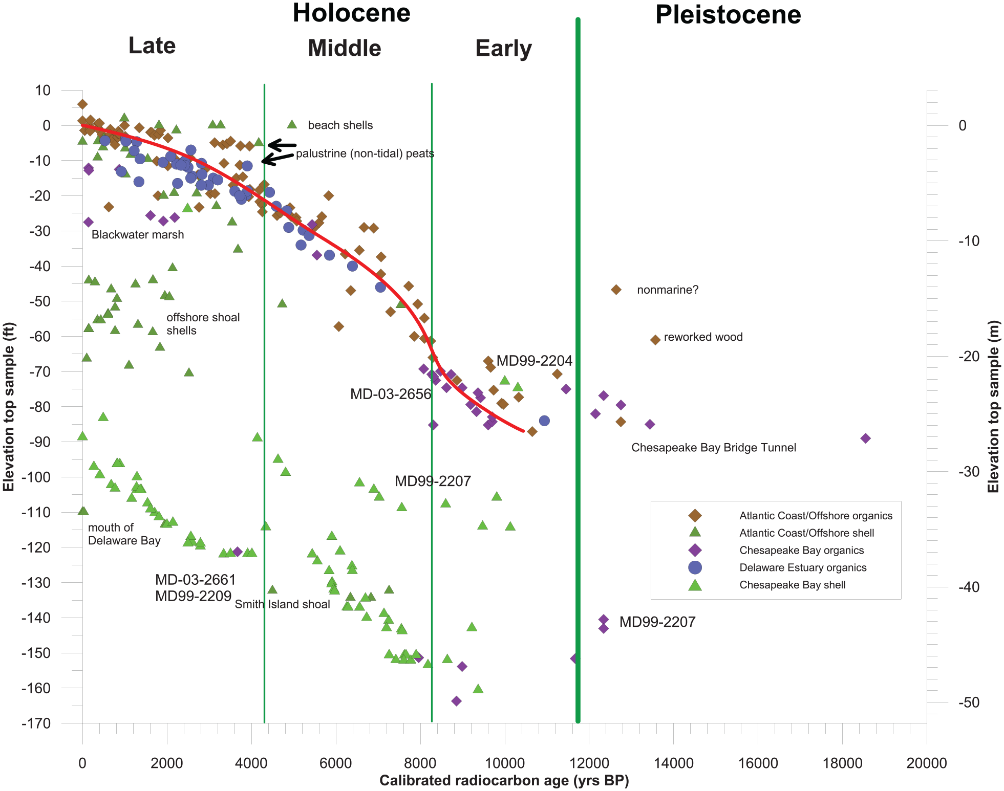
Age versus sample elevation plot of marine and estuarine radiocarbon dates from shell and organic plant material from the Delmarva Peninsula region. Red line is an approximate sea-level rise curve based on these data. Specific samples or groups of samples referred to in the paper are indicated by text on plot.

Analysis

U.S. Mid-Atlantic Holocene marine, estuarine, and non-marine deposition and the radiocarbon record

Radiocarbon dates from estuarine and marine sediments are a measure of Holocene sea-level rise and sedimentation typically associated within single geographic or geomorphic entities (Nikitina et al., 2015, Chesapeake Bay-Cronin et al., 2019). A plot of radiocarbon dates relative to their elevation from the fringing estuarine and marine deposits (Figure 2) incorporates dates from Chesapeake Bay, Delaware Bay, and the Atlantic Coast and offshore. The plot includes previously unreported dates and dates related to possible Holocene neotectonic influences (DeJong et al., 2015; Harrison et al., 1965). Late-Holocene marsh dates from Chesapeake Bay (Cronin et al., 2019) and Delaware Bay (Nikitina et al., 2014, 2015) related to late-Holocene sea-level fluctuations at a finer scale than is the focus of this paper are not included.

A few late Pleistocene dates are included in Figure 2. These include two outlier dates, one of which is a piece of wood from an offshore core with other dates that fall within a middle Holocene cluster, another from a core offshore of Maryland that could be from a non-marine organic deposit. Other late Pleistocene (and earliest Holocene) dates from geotechnical borings for the Chesapeake Bay Bridge Tunnel construction were reported by Harrison et al. (1965).

Estuarine and marine organic material dates

Dated organic material includes sediment, wood, peat, and marsh plants but excludes shell. These dates form the basis for most sea-level studies (Cronin et al., 2019; Nikitina et al., 2000). This is because plant material derived from marshes or adjacent swamps is deposited at or near sea level, providing an approximate date for the elevation from which the sample was taken. Figure 2 includes dates from the offshore and coastal Atlantic of the Delmarva and Chesapeake and Delaware Bays.

As would be expected, the Holocene dates track the rise of sea level (Figure 2). The curve is not a statistical calculation, but rather an approximate curve drawn roughly at the mid-point of the distribution of dates. Determining a statistical “sea-level curve” is not prudent, given the variability of accuracy of the elevations of the tops of offshore cores (Mattheus et al., 2019) and estimates of land-surface elevation from topographic maps with five-foot contour intervals for older data. Holocene sea-level rise was most rapid at the early to middle Holocene boundary (between 9 and 7 ka BP), with rates as high as 1 m/100 years. Rate of sea-level rise slows after 7 ka and rises at a consistent rate of 0.25 m/100 years and then falls to 0.2 m/100 years for the latest Holocene.

Estuarine and marine shell dates

Shell radiocarbon dates are binned into five groups (based on sampling location): beach shells, estuarine or shallow marine deposit shells, offshore shoal shells, deeper water shells from the mouths of Delaware and Chesapeake Bays, and Chesapeake Bay estuarine thalweg shells (Figure 2). Holocene shell dates from Delmarva Atlantic beaches are primarily late-Holocene in age, with only one middle Holocene outlier date. Shells that plot just below the cluster of organic deposits and track the rise of sea level during the Holocene are from nearshore or lagoonal deposits. These dates are also primarily late-Holocene in age, with only two from the middle Holocene. A cluster of dates in the late-Holocene from elevations between −40 ft (−12 m) and −70 ft (−21 m) are derived from cores across offshore shoal deposits. Shells from the deeper waters near the mouth of Delaware Bay are also late-Holocene in age, while those from the mouth of Chesapeake Bay (Smith Island Shoal) are middle Pleistocene in age. The final group of dates are from deep cores (MD03-2661, MD99-2207, MD99-2209, MD03-2656) in Chesapeake Bay (Colman et al., 2002; Willard et al., 2005). The earliest dates occur in the late early Holocene and continue throughout the Holocene. Corresponding sample elevations track the rise of sea level at consistent depths at the time of deposition, although the water-depth preference of the shell species dated (Mulinia) is assumed given the lack of variability of the core sediment (mud). Mulinia presently occupies a wide range of depths in estuaries, from intertidal to more than 7 m (Walker and Tenore, 1984).

Non-marine deposits

Radiocarbon dates from swamps, bogs, and Carolina Bays (Figure 3) record non-marine organic deposition on the uplands and coastal and offshore areas prior to sea-level transgression. These deposits are particularly climate-sensitive due to their dependence on rainfall to sustain environments wet enough to produce and preserve organic deposition. Small swamps and bogs are located adjacent to Holocene streams (Pizzuto and Rogers, 1992) and in isolated patches on the uplands where the seasonal water table is near the land surface. The largest wetland area is Cypress Swamp, which is located along the Delaware-Maryland border in the center of the Delmarva Peninsula. Deposition of bog sediments in the swamp (sphagnum-dominated with few arboreal pollen) began in the late Pleistocene and continued throughout the Holocene (Andres and Howard, 2000). Late Pleistocene sphagnum bog deposits like Cypress Swamp transitioned to more arboreal-dominated swamp deposits in the Holocene.

Figure 3.

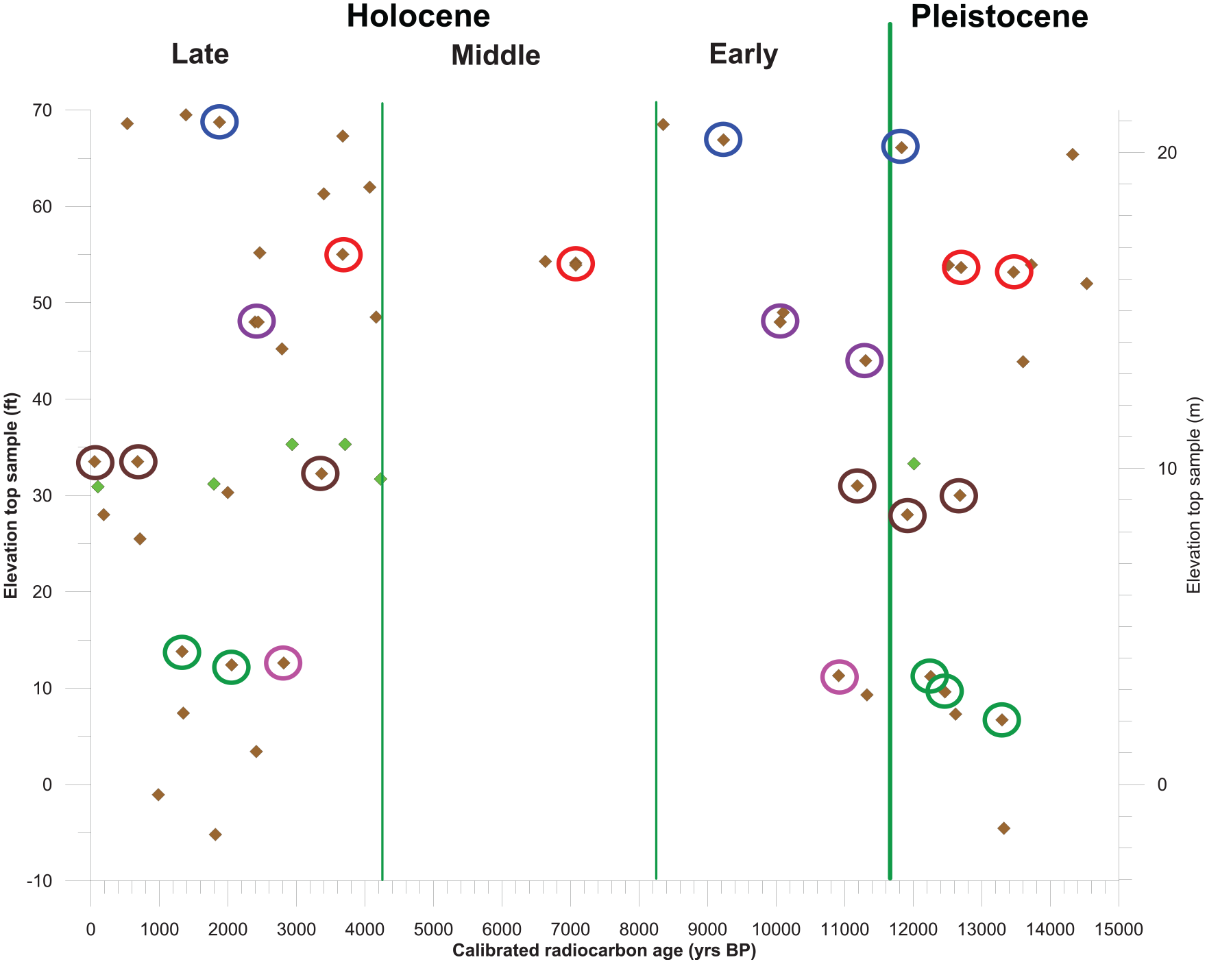
Plot of non-marine organic dates from the uplands of the Delmarva Peninsula. Green symbols are from the Cypress Swamp Formation. Brown symbols are from Carolina Bays. Color circles indicate samples that came from the same core in a Carolina Bay.

Carolina Bays are widespread on the Delmarva Peninsula, central Delaware, and adjacent Maryland (Stolt and Rabenhorst, 1987; Tomlinson and Ramsey, 2014). These circular depressions were present in the late Pleistocene, as suggested by radiocarbon dates from organic deposits as old as 25 ka BP (DGSRCD). Webb et al. (1994) conducted a pollen study on a Carolina Bay in central Delaware. They concluded from closely-spaced core samples that there was a depositional hiatus between the late Pleistocene and the middle Holocene. Radiocarbon dates from a more comprehensive set of onshore samples (Figure 3) indicates that deposition in Carolina Bays and in the Cypress Swamp was continuous throughout the late Pleistocene until about 11 ka BP. Deposition became sporadic over the rest of the early Holocene in Carolina Bays and sparse by the middle Holocene (Figure 3). Swamp deposition became widespread both in the Cypress Swamp and Carolina Bays at the middle to late-Holocene boundary and has been continuous ever since.

U. S. Mid-Atlantic Holocene climate record

Boundaries of the Holocene subepochs occur at climatic events with a global signal (Walker et al., 2019). Teasing out local from regional climate signals is a challenge and matching local or regional changes to global ones even more so. One of the purposes of this study is to determine if global climate signals can be recognized in the Delmarva Peninsula region of eastern North America. Syntheses of Holocene climate variability for eastern North America include pollen records from lakes and ponds (Shuman and Burrell, 2017; Shuman and Marsicek, 2016), stable isotopes from lakes and estuaries (Cronin et al., 2005; Mullins et al., 2011; Zhao et al., 2010), radiocarbon dates and soil profiles from floodplains (Lombardi et al., 2020; Stinchcomb et al., 2012), and Native American cultural changes (Fiedel, 2014). These syntheses show that the climate fluctuated between wet and dry and/or warm and cool periods and that there may have been a periodicity to some of this variability. Many of the data sets also reflect the major global climate shifts used for the early-middle (8.2 ka BP) and middle-late (4.25 ka BP) Holocene boundaries (Walker et al., 2019). The Holocene Climatic Optimum (HCO) was a warm period (1–2°C increase in summer temperatures) whose timing depended upon a region’s spatial relationship to the Laurentide Ice Sheet (Renssen et al., 2012). For eastern North America, this occurred between 5 and 7 ka (Renssen et al., 2012). The last cooling event was the Medieval Climate Anomaly (MCA) that occurred between 0.7 and 0.15 ka BP (1200–1800 AD; Wanner et al., 2011). Some reports break out the Little Ice Age (LIA) from the MCA for the period from 1400 to 1900 AD (Cronin et al., 2019; Lombardi et al., 2020).

Figure 4 shows a selection of the regional climate records of relevance to the Delmarva Peninsula. The most complete Delmarva Holocene climate record is from pollen and radiocarbon dates from Chesapeake Bay estuarine sediments (Cronin et al., 2005; Willard et al., 2003, 2005). A proxy climate curve was constructed using Pinus pollen percentages, the only pollen genera with statistically significant changes across vertical sections in core (Willard et al., 2005). Willard et al. (2005) noted eight events where Pinus percentages changed significantly; these were correlated with regional climatic changes that were significant enough to affect the flora (0 through 6 on Figure 4). Regional palynological studies have noted the decline of Tsuga (hemlock) during the Holocene. Booth et al. (2012) analyzed the data for the mid-Atlantic and concluded that the timing of Tsuga decline, between 5.4 and 5 ka BP, was variable depending on local factors. Tsuga populations throughout the region generally underwent three phases: (1) Robust populations in the early Holocene; (2) A period of rapid decline in population percentages at around 5 ka BP; and (3) A persistent decline in populations over the late-Holocene. Booth et al. (2012) concluded that climate changes played a role in Tsuga population shifts; however, they cannot tie the rapid mid-Holocene decline to an “event.” Willard et al. (2005) document a middle Holocene Tsuga decline in Chesapeake Bay cores at about the same time as that reported by Booth et al. (2012).

Figure 4.

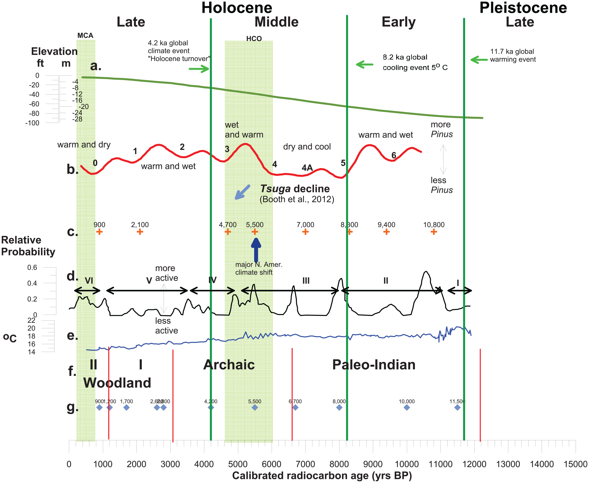
Mid-Atlantic and Delmarva region climate records. Climate events-the Holocene climate optimum (HCO), and the Medieval Climate Anomaly (MCA) are shown as shaded boxes and taken from Lombardi et al. (2020). The numbers in record b are the Pinus phases of Willard et al. (2005). The Roman numerals in record d are the climate phases of Stinchcomb et al. (2012): (a) Delaware Sea Level Curve (Nikitina et al., 2000), (b) Pinus percentages Chesapeake Bay (Willard et al., 2005), (c) N. American climate shifts (Shuman and Marsicek, 2016), (d) Mid-Atlantic fluvial activity (Lombardi et al., 2020; Stinchcomb et al., 2012), (e) SST Va slope core CH-07-98 (Sachs, 2007), (f) Native American cultures (Custer, 1987) and (g) Native American point style changes (Fiedel, 2014).

Sachs (2007) reported cooling of sea surface temperatures (SST) during the Holocene at core CH07-98-GCC19 on the Atlantic slope off the mouth of Chesapeake Bay (Figure 4). The author proposed that a shifting Gulf Stream and rising sea level may account for some of the cooling, but that additional modeling was needed to determine causality.

Lombardi et al. (2020) compiled Holocene radiocarbon dates from floodplain deposits in eastern North America and created probability curves of fluvial activity by summing ¹⁴C probability functions generated during the calibration process. Multiple dates were compiled for the mid-Atlantic region, primarily from the Delaware and Susquehanna River watersheds, and a probability curve of fluvial activity was plotted. Lombardi et al. (2020) concluded that chronologies of fluctuation between alluvial deposition and landscape stability could be determined and that the Holocene activity was not cyclical nor synchronous between watersheds. They also concluded that fluvial activity was more spatially restricted during warm and dry climatic conditions than cooler and wetter conditions. The significance of the fluvial activity to this study is that it presents a climate signal in the watersheds that ties the Delmarva Peninsula to a sediment input variability signal (e.g. higher activity equals greater sediment input into the system; stability equals less sediment input into the system). Lombardi et al. (2020) also considered major climatic events, early Holocene meltwater pulses (MWP), the late middle Holocene climate optimum (HCO), and the late-Holocene Medieval climate anomaly (MCA; Figure 4).

Figure 4 also includes the Native American culture divisions used by archeologists on the Delmarva Peninsula (Custer, 1989) and shifts in point culture (i.e. shapes and manufacture of arrowheads and other projectile points) for the mid-Atlantic (Fiedel, 2014). Fiedel documents multiple changes in Native American point culture in the mid-Atlantic during the Holocene, many regional in nature and occurring over short (decadal) time spans; the timing of these major shifts is noted in Figure 4. Fiedel (2014) directly attributes these culture shifts to regional climate and vegetation changes that affected game populations. Changes in game populations required hunting adaptations, hence the point re-design. Although little else regarding Native American culture is referenced in this paper, it is important to recognize that the Holocene changes, whether driven by sea-level rise or climate, had an impact upon the inhabitants of the Delmarva Peninsula.

U.S. Mid-Atlantic dates as a climate indicator

Radiocarbon dates provide a record of when two types of carbon-bearing organic material were deposited: (1) mollusk shells preserved in estuarine and marine sediments; and (2) plant material deposited primarily in marsh, swamp, or bog sediments. All environmental factors being equal, such as climate and sedimentary dynamics of respective depositional environments, there should have been persistent marine, estuarine, marsh, swamp, or bog deposition throughout the epoch within the Delmarva region, and therefore, an even distribution of radiocarbon dates. If an even distribution does not exist, then erosion or lack of deposition occurred. The most likely scenarios are that sea-level rise outpaced sedimentation rate (Cronin et al., 2007) or drought prevented deposition in freshwater settings (Webb, 1990; Webb et al., 1994).

Assuming persistent organic deposition throughout the Holocene, or that deposition was controlled by mitigating factors (erosion or climate), was sampling and dating of samples sufficient to capture the periods of organic deposition? There are no non-marine lacustrine deposits to provide a complete Holocene record in this region. Aside from Chesapeake Bay estuarine cores (Colman et al., 2002; Cronin et al., 2005), no robust series of dates from a single core exists. Rather, this study relies largely upon hundreds of dates from widespread locations. The following factors substantiate that the data are sufficient to have captured the Holocene record of organic deposition. First, the entire thickness of the Holocene was penetrated and basal Holocene deposits were sampled for radiocarbon analysis. This is important for demonstrating that sea-level rise patterns for the Delaware Bay and Atlantic Coast are consistent with those of the Chesapeake Bay (Cronin et al., 2019). Second, where non-marine deposits were sampled, especially the Carolina Bays (Stolt and Rabenhorst, 1987; Webb, 1990; Webb et al., 1994), the data are consistent between multiple basins with late Pleistocene and early Holocene dates, few to no dates in the middle Holocene, and deposition returning in the late-Holocene (Figure 3). The pattern is also observed in the Cypress Swamp deposits. Third, radiocarbon dates from mollusk shells in deep Chesapeake Bay and offshore Atlantic cores are consistent with the depositional history of the estuarine and marine deposits interpreted from core and geophysical data (Mattheus et al., 2020a, 2020b). Fourth, outlier dates in all settings are few and can be explained by the reworking of older wood or shells into younger sediments. Although there are a few age reversals in core (older over younger dates), they are rare. Finally, the radiocarbon dataset bears out regional sea-level records and climate signals from sources and settings. Timing of prolonged periods of drought and temperature fluctuations observed in pollen records are mirrored by the preservation or lack of organic deposits at other sites. Likewise, the timing and rates of sea-level rise, as tracked by dates of coastal deposits, are supported by multiple dates independent of those from which the sea-level curves were constructed.

Results and discussion

Delmarva radiocarbon record and Holocene climate and depositional history

The marine and estuarine radiocarbon dates from the Delmarva (Figure 2) illustrate the rise of sea level during the Holocene. Rates of sea-level rise were greatest between 9 and 7 ka, spanning the early to middle Holocene boundary in agreement with observations for Chesapeake Bay (Cronin et al., 2007). Rates of rise were consistent throughout the middle Holocene and decreased at about 3 ka, consistent with Nikitina et al. (2000) sea-level curve for Delaware. Dates from mollusk shells (Mulinia) from Chesapeake Bay cores (Colman et al., 2002; Willard et al., 2005) likewise track sea-level rise throughout at depths below the sea-level curve consistent with the present water depths of the tops of the cores. Sedimentation rate kept pace with sea-level rise in the deeper portions of the Chesapeake estuary through the Holocene. In the middle Holocene, there is a condensed section in the cores between about 6.5 and 3.5 ka, starting and ending earlier down the bay (MD99-2207) than farther up the estuary (MD-03-2661, MD99-2209). Cronin et al. (2005) attribute the condensed zone to low sedimentation rates and possible erosion, but do not discuss causality.

Almost all shells from the Atlantic nearshore (⩽8 m) and from deeper waters (⩾12 m) are of late-Holocene age. Shells in deeper water are sourced almost entirely from sandy shoal deposits (Mattheus et al., 2020a, 2020b) and indicate that the shoals are late-Holocene in age. Shell deposition during the early and middle Holocene is inferred to have been absent to rare and any indication of reworking of older Holocene shells into younger Holocene deposits is lacking. The lack of middle and early Holocene shells is attributed to the higher rates of sea-level rise and the concurrent drowning of the shelf landscape with little associated offshore sedimentation. In the late-Holocene, offshore sedimentation is interpreted to have stabilized with lower rates of sea-level rise; shoals subsequently formed in response to storms reworking older sandy deposits such as the Beaverdam Formation (Mattheus et al., 2020a, 2020b). It must be noted that most of the shell dates are from the Delaware offshore. The few dates off Maryland and Virginia that represent comparable water depths cluster with the corresponding Delaware dates. The few dates from the middle Holocene are from deeper waters (⩾40 m) off the mouth of Chesapeake Bay, across the Smith Island shoal.

Deposition and preservation of organic material, especially from non-marine deposits, are more sensitive to atmospheric climate change (temperature and rainfall shifts) than marine and estuarine mollusks, which are more sensitive to water temperature and salinity conditions. The Delmarva climate record from radiocarbon dates of organic materials was assessed against the climate interpretations based on Chesapeake Bay pollen records (Willard et al., 2005) and floodplain activity records from Delmarva Peninsula inland drainage basins (Lombardi et al., 2020) (Figure 4). Organic material dates from coastal marshes and estuaries (Figure 5a) and those from non-marine deposits (Figure 5d), as plotted against sample elevation, are compared with the Pinus abundances of Willard et al. (2005); Figure 5b) and fluvial activity based on work by Lombardi et al. (2020; Figure 5c). The non-marine dates (Figure 5d) are also depicted in an abundance bar chart that bins the dates into 500 year intervals as an alternative for assessing the Holocene distribution of non-marine dates (Figure 5e). The key depositional and climatic elements of Willard et al. (2005) and Lombardi et al. (2020) are summarized in Figure 2. The Holocene of the Delmarva for this discussion is divided into six phases that correspond to a modified version of those by Stinchcomb et al. (2012), given additional consideration of more recent work by Lombardi et al. (2020), Willard et al. (2005), and the radiocarbon dates from this study.

Figure 5.

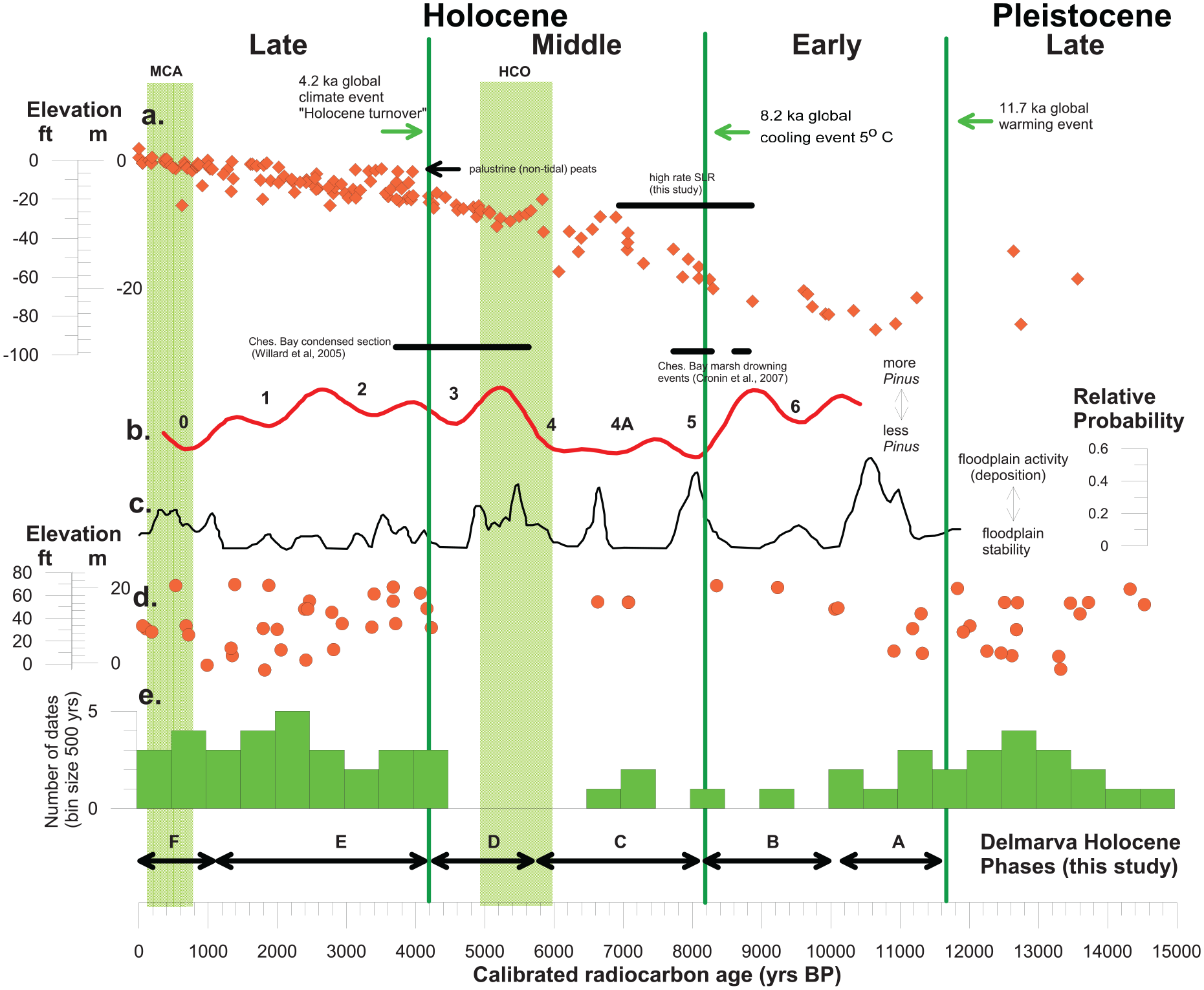
Summary of Delmarva region climate records and plots of plots of radiocarbon dates from organic material from coastal and estuarine deposits (sea-level signal) and upland deposits (climate signal): (a) coastal and estuarine radiocarbon dates (this study) plotted against sample elevation as a proxy for sea-level rise (this study), (b) Chesapeake Bay Pinus abundance curve (Willard et al., 2005), (c) mid-Atlantic fluvial activity (Stinchcomb et al., 2012), (d) upland organic radiocarbon dates plotted against sample elevation (this study), and (e) bar graph of number of dates (this study) in d plotted in 500-year bins.

Phase A: Late Pleistocene-early Holocene (>10 ka)

Lombardi et al. (2020) indicate that the cool and dry period from late Pleistocene to earliest Holocene time (Figure 5c) in the Delaware watershed was accompanied by periglacial braided stream deposition in the Delaware watershed (Phase I of Stinchcomb et al., 2012; Figure 4d). The boundary of Phase A, at 10 ka BP, is placed at the end of this depositional phase, the beginning of the Pinus minimum 6 of Willard et al. (2005) (Figures 4d and 5b), and the approximate timing of onset of the first estuarine deposition within the Chesapeake Bay sediments (Figure 2). Late Pleistocene organic deposition on the uplands (Figure 5d and e) was active, with a majority of the radiocarbon dates originating from Carolina Bays of the central Delmarva. Pollen data (Webb et al., 1994) indicate that the landscape at the time was a forest tundra dominated by Picea, Betula, Tsuga, and Pinus, with a mixture of shrubs and wet meadows (bogs) with tall herbs such as Sanguisorba. Harrison et al. (1965) reported a similar pollen assemblage at the mouth of what is now the Chesapeake Bay with the presence of sphagnum. At this time, the shoreline of the Atlantic Ocean was at approximately −30 m (−100 ft) and 30 to 50 km east of the present location (Figure 1). Estuarine deposition likely extended up the deeply incised valleys of the Susquehanna and Delaware at this time. The periglacial landscape, including late Pleistocene periglacial bogs, likely extended across the shelf to the lowstand shoreline (Finkelstein, 1986; unpublished DGS data).

Phase B: Early Holocene (10 to 8.2 ka)

The period between 10 ka and the end of the early Holocene (8.2 ka) marked the beginning of the encroachment of sea level with estuarine deposition in the major estuaries and in some tributaries along the Atlantic Coast. By the beginning of Phase B, organic deposition in the upland wetlands had become less common (Figure 5d and e). Webb et al. (1994) note a significant hiatus in core, both in the core itself and in the pollen record, between the earliest Holocene and the late-Holocene in the Carolina Bays. The observed hiatus is supported by the distribution of radiocarbon dates in this report (Figures 3, 5d and e). The flora at this time shifted to Pinus-dominated forest (Pinus minimum 6, Willard et al., 2005). Cool and dry conditions existed across the drainage basin (Phase II of Lombardi et al., 2020; Stinchcomb et al., 2012) and promoted a stable fluvial landscape.

Phase C: Middle Holocene (8.2 to 5.6 ka)

Phase C begins in the early to middle Holocene at 8.2 ka BP. A significant cold event (Wanner et al., 2011), which marks the boundary between the early to middle Holocene (Walker et al., 2019), coincides with several events in the Delmarva region. Sea-level rise increased to its highest Holocene rates (up to 1 m/100 years; Figures 2 and 5a; Cronin et al., 2007). Major paleovalleys flooded rapidly and peripheral terraces were being inundated, resulting in the widespread expansion of marshes (Cronin et al., 2007). On the Atlantic side, the shoreline rapidly transgressed across the landscape. Where interfluves were flooded, the shoreline migrated at rates of up to 3 km in 200 years (Mattheus et al., 2020b). Sea-level rise was rapid enough to preclude deposition of mollusk shells in shoals (Figure 2). A significant decline in Pinus percentages is also recorded in estuarine sediments, which is interpreted as a cooling event with a drop in temperatures of up to 3°C (Willard et al., 2005). In the drainage basin, this period is recognized by floodplain scouring and deposition of coarse-grained flood deposits (Phase III of Stinchcomb et al., 2012).

Following the 8.2 ka event, Phase C is characterized as a time of relative stability with consistently low Pinus percentages, dry and cool climate conditions (Willard et al., 2005), and floodplain stability, with the exception of a depositional period around 6.6 ka (Lombardi et al., 2020). Sparse organic deposition on the uplands continued the trend of the late early Holocene (Figures 3, 5d and e). During this time of dry to very dry conditions on the uplands, most of the Carolina Bays and the Cypress Swamp were dry and organic deposition ceased or was not preserved (Webb et al., 1994). The end of Phase C coincides with a cold period between 6.5 and 5.9 ka BP, which preceded the HCO (Wanner et al., 2011). Sea-level rise rates dropped but were still higher than those of the late-Holocene.

Phase D: Middle Holocene (5.6 to 4.2 ka)

The boundary between Phase C and Phase D occurs at 5.6 ka BP, at the end of Pinus minimum 4. In the Delmarva region, there is a major shift from deciduous to mixed Pinus-deciduous forests at this time, along with a decrease in the rates of sea-level rise, and a depositional phase in the drainage basin (Lombardi et al., 2020). It also coincides with the timing of regional and local Tsuga decline (Booth et al., 2012; Willard et al., 2005) and a major North American climate shift (Shuman and Marsicek, 2016). At this time, sea level was between −9 and −6 m (−30 to −40 ft) and the shoreline was approaching its present position on the lower Delmarva. Interfluves off the Delaware coast were overtopped and lagoonal deposits emplaced within tributaries to the Delaware River estuary (Mattheus et al., 2020b). The marine conditions were still more erosive than depositional and mollusk shells were not yet present in marine deposits (Figure 2). This phase encompasses the condensed section seen in the lower Chesapeake Bay (MD99-2207) and the first half of the condensed section in the upper estuary (MD-03-2661, MD-2209; Figure 2). At this time, there was also a phase of fluvial deposition across the watershed (Lombardi et al., 2020; Figure 5c). No organic radiocarbon dates from the uplands are reported for this interval, indicating that conditions were dry, or that there was a lag in deposition. A lag may represent the time it would have taken for the groundwater table levels to rise, intersect the Carolina Bay depressions, and provide prolonged wet conditions for organic materials to accumulate. There is a couplet that comprises Phase D in both the pollen record (Willard et al., 2005) and the fluvial watershed record (Lombardi et al., 2020). A wet period is inferred to have existed between Pinus minima 4 and 3, with increased Pinus coinciding with a depositional phase in the drainage basin (Figure 5b and c). The second part of the couplet is a Pinus minima (3), coinciding with a period of fluvial stability, indicative of a drier and cold period between 4.8 and 4.5 ka BP (Wanner et al., 2011).

Was Phase D the result of the HCO? The HCO varied in its timing across North America with a broad range of 7 to 5 ka BP in eastern North America (Renssen et al., 2012). At about 5.2 ka BP, Atlantic sea-surface temperatures off the mouth of Chesapeake Bay shifted from stability during the early and middle Holocene to a steady decrease through the rest of the middle and the late-Holocene (Sachs, 2007; Figure 4e). Lombardi et al. (2020) limit the HCO to 6 to 4.6 ka (Figure 4). Willard et al. (2005) describe this time as one of regional Pinus increase to the north and an increase in mid-Atlantic January warming of 2–4°C based on pollen calibration. Stinchcomb et al. (2012) indicate this time interval to be a period of warm and dry conditions in the drainage basin with a period of incision and stability between 5 and 6 ka BP. There is a likely correlation between Phase D and the HCO between about 6 and 5 ka BP (Figure 5), whereby the dry period indicated by Pinus minima 3 and fluvial stability (Figure 5b and c) mark the end of the HCO and a shift into the late-Holocene climate.

Phase E: Late-Holocene (4.2 to 1.1 ka BP)

The boundary between Phase D and Phase E is at the middle and late-Holocene boundary (~4.2 ka BP). The boundary coincides with a further decrease in the rate of sea-level rise to near its current 0.3 m/100 years. It also marks the renewal of organic deposition on the uplands (Figure 5d and e), the appearance of palustrine (non-tidal) peats in the Delaware estuary tributaries (Figure 5a; Pizzuto and Rogers, 1992), and the beginning of a period of long-term fluvial stability in the drainage basin (Figure 4d; end of Phase IV and Phase V of Stinchcomb et al., 2012). By the beginning of the late-Holocene, marine and estuarine conditions had occupied their present extents (Figure 2). Water depths also promoted the accumulation of shoal deposits stable enough to allow marine mollusk productivity to increase (Figure 2). Non-tidal palustrine deposits appeared in the tributaries to Delaware Bay due to the effects of rising sea levels into the stream valleys (Pizzuto and Rogers, 1992). Marsh deposition expanded on the periphery of both Delaware (Nikitina et al., 2015) and Chesapeake Bay (Cronin et al., 2019). Widespread wetland deposition in the uplands returned in the Carolina Bays and Cypress Swamp and continued throughout the late-Holocene (Figure 5a). Warm and wet conditions with mixed Pinus and deciduous forests lasted throughout Phase E with two Pinus minima (2 and 1), indicating drier periods in an overall wet time. Pinus percentages continued an overall decline that lasted throughout the rest of the late-Holocene (Figure 5b). Wanner et al. (2011) note a cold period between 3.3 and 2.5 ka BP and another at 1.75 to 1.35 ka BP, but it is unclear whether these events are reflected in the Delmarva depositional record.

Phase F: Late-Holocene (1.1 ka BP to present)

The boundary between Phase E and Phase F is at 1.1 ka BP, which is the beginning of Pinus minima 0 and a time of increased fluvial deposition in the drainage basin (Figure 5b and c). The end of the late-Holocene is noted for the Medieval Climate Anomaly (MCA) or the Little Ice Age (LIA) that had the coldest temperatures since the 8.2 ka BP event (Wanner et al., 2011). Although there is some indication of this event in the pollen record (end of Pinus minimum 0; Willard et al., 2005) and it coincides with a period of deposition in the watershed (Lombardi et al., 2020), it is also the period of European settlement. The effects of a cold period cannot always be separated from the legacy of settlement clearing and agricultural practices (Stinchcomb et al., 2012). By the beginning of Phase F, Atlantic and estuarine shorelines were near their present locations, widespread marshes were present along the estuaries with an average rate of sea-level rise of 1.26 mm/year (0.3 m or 1 ft/century; Cronin et al., 2019; Nikitina et al., 2015).

Conclusions

The Holocene of the U.S. Middle-Atlantic was a dynamic time of sea-level rise and climate variation that is recorded by radiocarbon dates of both mollusk shells and plant material. An integrated approach using both marine-estuarine and non-marine radiocarbon dates provides a complete record of the Holocene. The marine-estuarine dates capture the rise of sea-level with generally continuous deposition even during times of highest rates of sea-level rise during the early-middle Holocene transition. Non-marine dates are more sensitive to climate and record wet periods while times of sustained drought did not produce organic sediments that could be dated. This is especially true of Carolina Bays, where closely-sampled cores yielded radiocarbon dates with significant hiatuses that coincide with regional dry periods based on pollen and soil studies.

The wet and dry periods along with the sea-level curve substantiate the global subdivisions based on climatic shifts (Walker et al., 2019) and are applicable to the U.S. Mid-Atlantic. The late Pleistocene to early Holocene (Phase A) was a time of transition from periglacial climate and low sea levels to a much warmer climate with sea-level rise beginning to impact the area with estuarine deposition in the incised river valleys. This is the time of global temperature rise and shifts in atmospheric circulation (Buizert et al., 2014; Walker et al., 2019). The remainder of the early Holocene (Phase B) was a time of estuarine deposition in the incised valleys, reduced wetland deposition on the uplands, and a shift to a rapid rise of sea level. The early to middle Holocene boundary coincided with the highest rates of sea-level rise, rapid migration of the shoreline across the shelf, drowning of the terraces peripheral to the estuaries, and widespread reduction of wetland deposition on the uplands. The early-middle Holocene boundary at 8.2 ka (Walker et al., 2019) coincides with the Phase B-C boundary as marked by the rapid increase in sea-level rise, drowning of marshes (Cronin et al., 2007) and transition in the relatively dry period of the middle Holocene (Wanner et al., 2008).

These trends continued throughout the middle Holocene (Phases C and D), with dry conditions on the uplands and shoreline migration both on the Atlantic and along the estuary margins. The rate of sea-level rise decreased toward the end of the middle Holocene (Phase D) and there was a period of limited deposition in the deeper portions of the Chesapeake Bay estuary. The boundary between the middle and late-Holocene coincided with a climate shift that is well marked across the Delmarva Peninsula. Unlike the record from mid-latitude North America where widespread drought was recorded (Shuman and Marsicek, 2016), the late-Holocene in the mid-Atlantic appears to have been more equitable with continuous deposition of organic material on swamps in the uplands. Sea-level rise slowed to its present rates of 0.3 m/century. Offshore Atlantic deposition saw the development and stabilization of shoals, which incorporated mollusk shells. There was expansion of the marshes and palustrine deposition in the non-tidal portions of the stream valleys. The middle/late boundary in particular is well-represented in the radiocarbon date record of the region. The early/middle boundary is less evident but the rapid rise of sea level, coincident with the event, is recorded by organic materials from marshes and estuaries. Climatic events such as the Holocene Climatic Optimum and the Medieval Climate Anomaly (including the Little Ice Age) cannot be discerned by the radiocarbon record alone.

The early-middle-late subdivisions of the Holocene (Walker et al., 2019) proved to be useful in outlining the Holocene geologic history of the U.S. Mid-Atlantic. A similar approach of combining marine/non-marine datasets in a coastal region could be fruitful in documenting in detail the intersection of sea-level rise and non-marine settings. This intersection could prove to be an important tool for the Holocene history of human habitation of not only eastern North America but of any coastal setting. Habitation patterns were influenced by the transgressive shorelines associated with sea-level rise and by climate shifts from wet to dry with the migrations that followed to access fresh water resources. Understanding the dynamic sea, estuarine, and climate changes that affected the Delmarva Peninsula over the Holocene, is of use not only to the geologic community, but also to archeologists involved in the chronology of Native American culture changes and habitation.

Supplemental Material

sj-xlsx-1-hol-10.1177_09596836211048282 – Supplemental material for A radiocarbon chronology of Holocene climate change and sea-level rise at the Delmarva Peninsula, US Mid-Atlantic Coast

Supplemental material, sj-xlsx-1-hol-10.1177_09596836211048282 for A radiocarbon chronology of Holocene climate change and sea-level rise at the Delmarva Peninsula, US Mid-Atlantic Coast by Kelvin W Ramsey, Jaime L. Tomlinson and C. Robin Mattheus in The Holocene

Footnotes

Acknowledgements

This paper is dedicated to the memory of John C. (Chris) Kraft for his contribution to the understanding of Holocene depositional environments, sea-level rise, and the relationship between antecedent topography and preservation of Holocene deposits. Without his foundational work and that of his students at the University of Delaware, including recognition of the importance of radiocarbon dating, this study would not be possible.

Funding

Funding for radiocarbon dates contracted by the Delaware Geological Survey came from internal project funding, the USGS Statemap geologic mapping program (G10AC00389, G11AC20261, G12AC20231, G13AC00174, G15AC00217, and the BOEM Cooperative (M14AC00003) and ASAP (Atlantic Sand Assessment Program; M16AC00001) projects.

ORCID iD

Kelvin W Ramsey

Supplemental material

Supplemental material for this article is available online.

References

Andres

Howard

(2000) The Cypress swamp formation, Delaware. Delaware Geological Survey report of investigations No 62, 13 p. Newark, DE: University of Delaware.

Booth

Brewer

Blaauw

et al. (2012) Decomposing mid-Holocene Tsuga decline in eastern North America. Ecology 93: 1841–1852.

Buizert

Gkinis

Severinghaus

, et al. (2014) Greenland temperature response to climate forcing during the last deglaciation. Science 345: 1177–1180.

Childers

Madsen

Krantz

, et al. (2019) Constraining the geometry of subsurface paleochannels beneath Delaware Bay and the Mid-Atlantic inner continental shelf. Journal of Coastal Research 35: 590–599.

Chrzastowski

(1986) Stratigraphy and geologic history of a holocene lagoon system: Rehoboth Bay and Indian River Bay, Delaware. PhD Dissertation, University of Delaware, Newark, DE.

Colman

Baucom

Bratton

, et al. (2002) Radiocarbon dating, chronologic framework, and changes in accumulation rates of Holocene estuarine sediments from Chesapeake Bay. Quaternary Research 57: 58–70.

Colman

Halka

Hobbs Ill

, et al. (1990) Ancient channels of the Susquehanna river beneath Chesapeake Bay and the Delmarva Peninsula. Geological Society of America Bulletin 102: 1268–1279.

Colman

Mixon

(1988) The record of major quaternary sea-level changes in a large coastal plain estuary, Chesapeake Bay, Eastern United States. Palaeogeography, Palaeoclimatology, Palaeoecology 68: 99–116.

Costas

Ferreira

Plomaritis

, et al. (2016) Coastal barrier stratigraphy for Holocene high-resolution sea-level reconstruction. Nature Scientific Reports 6: 38726.

10.

Cronin

Clevenger

Tibert

, et al. (2019) Holocene sea-level variability from Chesapeake Bay tidal marshes USA. The Holocene 29: 1679–1693.

11.

Cronin

Thunell

Dwyer

, et al. (2005) Multiproxy evidence of Holocene climate variability from estuarine sediments, eastern North America. Paleoceanography 20: PA4006.

12.

Cronin

Vogt

Willard

, et al. (2007) Rapid sea level rise and ice sheet response to 8,200-year climate event. Geophysical Research Letters 34: L20603.

13.

Custer

Griffith

(1987) Palynology and stratigraphy of the Mitchell Farm site (7NC-A-2), and the Dill Farm site (7K-E-12), Delaware. University of Delaware Center for archaeological research report no. 4, 22 p. Newark, DE: University of Delaware.

14.

Daniels

(1994) Late quaternary geomorphic setting of archaeological site 7k-C-107, Kent county, Delaware. M.S. Thesis, University of Delaware, Newark, DE.

15.

DeJong

Bierman

Newell

, et al. (2015) Pleistocene relative sea levels in the Chesapeake Bay region and their implications for the next century. GSA Today 25: 4–10.

16.

Edwards

(2007) Holocene Molluscan Aminochronology and time averaging in Chesapeake Bay Ssediments. M.S. Thesis, University of Delaware, Newark, DE.

17.

Fiedel

(2014) Abrupt changes of climate and point styles along the Atlantic seaboard of eastern North America: How were they connected? Archaeology of Eastern North America 42: 77–100.

18.

Field

(1981) Sediments, shallow subbottom structure and sand resources of the inner continental shelf, central Delmarva Peninsula. United states army corps of engineers technical paper no. 79–2, 124 p. Fort Belvoir, VA: Coastal Research Center.

19.

Finkelstein

(1986) The late quaternary evolution of a twin barrier-island complex, Cape Charles, Virginia. PhD Dissertation, Virginia Institute of Marine Science, College of William and Mary, Williamsburg, VA.

20.

Fletcher

Knebel

Kraft

(1990) Holocene evolution of an estuarine coast and tidal wetlands. Geological Society of America Bulletin 102: 283–297.

21.

Fletcher

Knebel

Kraft

(1992) Holocene depocenter migration and sediment accumulation in Delaware Bay: A submerging marginal marine sedimentary basin. Marine Geology 103: 165–183.

22.

Fletcher

Van Pelt

Brush

, et al. (1993) Tidal wetland record of Holocene sea-level movements and climate history. Palaeogeography, Palaeoclimatology, Palaeocology 102: 177–213.

23.

French

Millar

SWS

(2014) Permafrost at the time of the Last Glacial Maximum (LGM) in North America. Boreas 43: 667–677.

24.

Fruergaard

Andersen

Nielsen

, et al. (2015) High-resolution reconstruction of a coastal barrier system: Impact of Holocene sea-level change. Sedimentology 62: 928–969.

25.

Goettle

(1978) Geological development of the southern portion of Assateague Island, Virginia. MS Thesis, University of Delaware, Newark, DE.

26.

Groot

Jordan

(1999) The Pliocene and quaternary deposits of Delaware: Palynology, ages, and paleoenvironments. Delaware Geological Survey report of investigations no. 58. Newark, DE: University of Delaware.

27.

Harrison

Malloy

Rusnak

, et al. (1965) Possible late Pleistocene uplift Chesapeake Bay entrance. The Journal of Geology 73: 201–229.

28.

Hobbs

(2004) Geological history of Chesapeake Bay, USA. Quaternary Science Reviews 23: 641–661.

29.

Jengo

(1999) Hydrostratigraphy of the Cretaceous-age Potomac, Raritan, Magothy, and Merchantville FMS and Holocene-age DE river alluvium, Gloucester County. Northeastern Geology and Environmental Science 21: 148–178.

30.

Jengo

(2006) Stratigraphy and radiocarbon dates of Pleistocene and Holocene-age deposits, Delaware County, Pennsylvania-rectifying the presence of the Cape May formation and the Trenton gravel in the Delaware Valley. Northeastern Geology and Environmental Sciences 28: 45–76.

31.

Jengo

McLaughlin

Ramsey

(2013) Subsurface geology of the area between Wrangle Hill and Delaware City, Delaware. Delaware Geological Survey report of investigations no. 78. Newark, DE: University of Delaware.

32.

John

Pizzuto

(1995) Accelerated sea level rise 2,000 year BP in the Delaware Bay: Stratigraphic evidence from the Leipsic River Valley, Delaware USA. Journal of Coastal Research 11: 573–582.

33.

Knebel

Fletcher

Kraft

(1988) Late Wisconsinan-Holocene paleogeography of Delaware Bay; a large coastal plain estuary. Marine Geology 83: 115–133.

34.

Kraft

(1971) Sedimentary facies patterns and geologic history of a Holocene marine transgression. Geological Society of America Bulletin 82: 2131–2158.

35.

Kraft

(1976) Radiocarbon dates in the coastal zone (eastern Atlantic coast of North America). Delaware sea grant technical report DEL-SG-19-76. Newark, DE: College of Marine Studies, University of Delaware.

36.

Kraft

Belknap

(1986) Holocene epoch coastal geomorphologies based on local relative sea-level data and stratigraphic interpretations of paralic sediments. In: Pirazzoli

Suter

(eds) Late quaternary sea-level changes & coastal evolution. Journal of Coastal Research 1: 53–59.

37.

Leorri

Martin

McLaughlin

(2006) Holocene environmental and parasequence development of the St. Jones estuary, Delaware (USA): Foraminiferal proxies of natural climatic and anthropogenic change. Palaeogeography, Palaeoclimatology, Palaeoecology 241: 590–607.

38.

Lombardi

Davis

Stinchcomb

, et al. (2020) Fluvial activity in major river basins of the eastern United States during the Holocene. The Holocene 30: 1279–1295.

39.

Maley

(1981) A transgressive facies model for a shallow estuarine environment. MS Thesis, University of Delaware, Newark, DE.

40.

Markewich

Litwin

Pavich

, et al. (2009) Late Pleistocene eolian features in southeastern Maryland and Chesapeake Bay region indicate strong WNW-NW winds accompanied growth of the Laurentide Ice Sheet. Quaternary Research 71: 409–425.

41.

Marx

(1981) A dynamic model for an estuarine transgression based on facies variants in the nearshore of western Delaware Bay. MS Thesis, University of Delaware, Newark, DE.

42.

Mattheus

Ramsey

Tomlinson

(2020a) Geologic map of offshore Delaware. Delaware Geological Survey geologic map series no. 25, scale 1: 40,000. Newark, DE: University of Delaware.

43.

Mattheus

Ramsey

Tomlinson

(2020b) The evolution of coastal-plain incised valleys over multiple glacio-eustatic cycles: Insights from the inner continental shelf of Delaware. Journal of Sedimentary Research 90: 1510–1526.

44.

Mattheus

Ramsey

Santoro

(2019) Evaluating continental shelf seabed-elevation changes from archived sediment-core records: Issues with vertical positioning and implications for integration with subsurface geophysics. Journal of Coastal Research 36: 41–53.

45.

Millard

(2014) Conventions for reporting radiocarbon determinations. Radiocarbon 56: 555–559.

46.

Mixon

(1985) Stratigraphic and geomorphic framework of uppermost Cenozoic deposits in the southern Delmarva Peninsula, Virginia and Maryland. US Geological Survey professional paper 1067-G. Reston, VA: US Geological Survey.

47.

Mullins

Patterson

Teece

, et al. (2011) Holocene climate and environmental change in central New York (USA). Journal of Paleolimnology 45(2): 243–256.

48.

Newman

Munsart

(1968) Holocene geology of the Wachapreague Lagoon, Eastern Shore Peninsula, Virginia. Marine Geology 6: 81–105.

49.

Nikitina

Kemp

Engelhart

, et al. (2015) Sea-level change and subsidence in the Delaware estuary during the last ∼2200 years. Estuarine Coastal and Shelf Science 164: 506–519.

50.

Nikitina

Kemp

Horton

, et al. (2014) Storm erosion during the past 2000years along the north shore of Delaware Bay, USA. Geomorphology 208: 160–172.

51.

Nikitina

Pizzuto

Schwimmer

, et al. (2000) An updated Holocene sea-level curve for the Delaware coast. Marine Geology 171: 7–20.

52.

Oaks

(1964) Post-Miocene stratigraphy and morphology, outer Coastal Plain, southeastern Virginia. PhD Dissertation, Yale University, New Haven, CT.

53.

Owens

Denny

(1978) Geologic map of Worcester County, Maryland. Maryland Geological Survey geologic map, scale 1:62,500. Baltimore, MD: Maryland Geological Survey.

54.

Owens

Denny

(1979) Upper Cenozoic deposits of the central Delmarva Peninsula, Maryland and Delaware. US Geological Survey professional paper 1067-A. Reston, VA: US Geological Survey.

55.

Pizzuto

Rogers

(1992) The Holocene history and stratigraphy of palustrine and estuarine wetland deposits of central Delaware. Journal of Coastal Research 8: 854–867.

56.

Pizzuto

Schwendt

(1997) Mathematical modeling of autocompaction of a Holocene transgressive valley-fill deposit, Wolfe Glade, Delaware. Geology 25: 57–60.

57.

Raff

Shawler

Ciarletta

, et al. (2018) Insights into barrier-island stability derived from transgressive/regressive state changes of Parramore Island, Virginia. Marine Geology 403: 1–19.

58.

Ramsey

(2010) Stratigraphy, correlation, and depositional environments of the middle to late Pleistocene interglacial deposits of southern Delaware. Delaware Geological Survey report of investigations No 76. Newark, DE: University of Delaware.

59.

Ramsey

Baxter

(1996) Radiocarbon dates from Delaware: A compilation. Delaware Geological Survey report of investigations no. 54. Newark, DE: University of Delaware.

60.

Ramsey

Tomlinson

(2012) Geologic map of the Bethany Beach and Assawoman Bay quadrangles, Delaware. Delaware Geological Survey geologic map No 18, scale 1: 24,000. Newark, DE: University of Delaware.

61.

Renssen

Seppä

Crosta

, et al. (2012) Global characterization of the Holocene thermal maximum. Quaternary Science Reviews 48: 7–19.

62.

Sachs

(2007) Cooling of northwest Atlantic slope waters during the Holocene. Geophysical Research Letters 34: L03609.

63.

Shideler

Ludwick

Oertel

, et al. (1984) Quaternary stratigraphic evolution of the southern Delmarva Peninsula coastal zone, Cape Charles, Virginia. Geological Society of America Bulletin 95: 489–502.

64.

Shuman

Burrell

(2017) Centennial to millennial hydroclimatic fluctuations in the humid northeast United States during the Holocene. Quaternary Research 88: 514–524.

65.

Shuman

Marsicek

(2016) The structure of Holocene climate change in mid-latitude North America. Quaternary Science Reviews 141: 38–51.

66.

Sirkin

Denny

Rubin

(1977) Late Pleistocene environment of the central Delmarva Peninsula, Delaware-Maryland. Geological Society of America Bulletin 88: 139–142.

67.

Stinchcomb

Driese

Nordt

, et al. (2012) A mid to late Holocene history of floodplain and terrace reworking along the middle Delaware River valley, USA. Geomorphology 169–170: 123–141.

68.

Stolt

Rabenhorst

(1987) Carolina Bays on the eastern shore of Maryland: II. Distribution and origin 1. Soil Science Society of America Journal 51: 399–405.

69.

Tomlinson

Ramsey

(2014) Stratigraphic, hydrologic, and climatic influences of the formation and spatial distribution of Carolina Bays in central Delaware. Geological Society of America Abstracts with Programs 46(2): 71.

70.

Toscano

Kerhin

Cronin

, et al. (1989) Quaternary stratigraphy of the inner continental shelf off Maryland. Maryland geological survey report of investigations No 50. Baltimore, MD: Maryland Geological Survey.

71.

Walker

Head

Lowe

, et al. (2019) Subdividing the Holocene series/epoch: Formalization of stages/ages and subseries/subepochs, and designation of GSSP’s and auxiliary stratotypes. Journal of Quaternary Science 34: 173–186.

72.

Walker

Tenore

(1984) Growth and production of the dwarf surf clam Mulinia lateralis (say 1822) in a Georgia estuary. Gulf and Caribbean Research 7: 357–363.

73.

Wanner

Beer

Buitikofer

, et al. (2008) Mid to late-Holocene climate change: An overview. Quaternary Science Reviews 27: 1791–1828.

74.

Wanner

Solomina

Grosjean

, et al. (2011) Structure and origin of Holocene cold events. Quaternary Science Reviews 30: 3109–3123.

75.

Webb

(1990) Late quaternary water-level fluctuations in the northeastern United States. PhD Dissertation, Brown University, Providence, RI.

76.

Webb

Newby

Webb

(1994) Palynology and paleohydrology of Delaware. In, Kellogg

Custer

(eds) Paleoenvironmental studies of the state route 1 corridor: Contests for prehistoric settlement, New Castle and Kent Counties. Delaware Department of Transportation Archaeology Series 114: 36–47.

77.

Wehmiller

York

Bart

(1995) Amino acid racemization geochronology of reworked quaternary mollusks on U.S. Atlantic Coast beaches: Implications for chronostratigraphy, taphonomy, and coastal sediment transport. Marine Geology 124: 303–337.

78.

Wells

(1994) Non-energy resources and shallow geological framework of the inner continental margin off Ocean City, Maryland. Maryland Geological Survey coastal and estuarine geology open file report no. 16. Baltimore, MD: Maryland Geological Survey.

79.

Whallon

(1989) The Holocene stratigraphy of three freshwater to oligohaline wetlands, Kent County, Delaware. MS Thesis, University of Delaware, Newark, DE.

80.

White

(1978) Influence of glacial meltwater in the Atlantic Coastal Plain. Southeastern Geology 19: 139–156.

81.

Wilke

Dalan

Walsh

, et al. (1980) Cultural resource survey of U.S. Naval reservation Bloodsworth Island, Dorchester County, Maryland. Geo Recon International report for Maryland historical trust, 111 p. Seattle, WA: Geo Recon International.

82.

Willard

Bernhardt

Korejwo

, et al. (2005) Impact of millennial-scale Holocene climate variability on eastern North American terrestrial ecosystems: Pollen-based climatic reconstruction. Global and Planetary Change 47(1): 17–35.

83.

Willard

Cronin

Verardo

(2003) Late-Holocene climate and ecosystem history from Chesapeake Bay sediment cores, USA. The Holocene 13: 201–214.

84.

Zhao

Ito

, et al. (2010) Holocene climate trend, variability, and shift documented by lacustrine stable-isotope record in the northeastern United States. Quaternary Science Reviews 29: 1831–1843.

Supplementary Material

Please find the following supplemental material available below.

For Open Access articles published under a Creative Commons License, all supplemental material carries the same license as the article it is associated with.

For non-Open Access articles published, all supplemental material carries a non-exclusive license, and permission requests for re-use of supplemental material or any part of supplemental material shall be sent directly to the copyright owner as specified in the copyright notice associated with the article.

0.00 MB

0.04 MB