Historical biogeographic range shifts and the influence of climate change on ocean quahogs ( Arctica islandica ) on the Mid-Atlantic Bight

Abstract

The Holocene, starting approximately 11.7 cal ka, is characterized by distinct periods of warming and cooling. Despite these known climate events, few temperature proxy data exist in the northwestern Atlantic Ocean. One potential record of past water temperatures is preserved in the marine fossil record. Shell growth of ocean quahogs (Arctica islandica), a long-lived bivalve, can provide records of past environmental conditions. Arctica islandica habitat includes the Mid-Atlantic Bight (MAB), an area rapidly warming as a consequence of climate change. The Cold Pool, a bottom-trapped water mass on the outer continental shelf within the MAB, rarely rises above 15°C. Ocean quahogs inhabiting the MAB are confined to the Cold Pool as a consequence of an upper thermal limit for the species of ~15–16°C. Recently, dead A. islandica shells were discovered outside of the species’ present-day range, suggesting that the Cold Pool once extended further inshore than now observed. Shells collected off the Delmarva Peninsula were radiocarbon-dated to identify the timing of habitation and biogeographic range shifts. Dead shell ages range from 4400 to 60 cal BP, including ages representing four major Holocene cold events. Nearly absent from this record are shells from the intermittent warm periods. Radiocarbon ages indicate that ocean quahogs, contemporaneous with the present MAB populations, were living inshore of their present-day distribution during the past 200 years. This overlap suggests the initiation of a recent biogeographic range shift that occurred as a result of a regression of the Cold Pool following the Little Ice Age.

Keywords

Cold Pool dark ages cold period Little Ice Age Neoglacial ocean quahog range shift

Introduction

Key climate events in the North Atlantic during the middle to late-Holocene include the Neoglacial Period (Jennings et al., 2002; Moossen et al., 2015), the Roman Warm Period (RWP) ( Wang et al., 2012), the Dark Ages Cold Period (DACP) (Helama et al., 2017), the Medieval Warm Period (MWP = Medieval Climate Anomaly) (Graham et al., 2011; Moossen et al., 2015), and the Little Ice Age (LIA; Moore et al., 2017; Moossen et al., 2015; Ogilvie and Jónsson, 2001). Since the end of the LIA the waters of the U.S. northeastern continental shelf have been in a cycle of warming and cooling periods, a consequence of the Atlantic Multidecadal Oscillation (AMO; Moore et al., 2017; Chen and Tung, 2018; Hou et al., 2019), superimposed on a persistent warming trend (Hanna et al., 2004; Wallace et al., 2018) well documented in the meteorology of the region (Auger et al., 2019). Recently, the Western North Atlantic has been warming at a rate faster than >90% of oceans around the world (Lentz, 2017; Pershing et al., 2015; Saba et al., 2016), likely due to a northward shift of the Gulf Stream (Neto et al., 2021; Sachs, 2007). Warming water alters bottom conditions, affecting the survival and distribution of benthic species on the US continental shelf (Friedland and Hare, 2007; Hofmann et al., 2018; Lucey and Nye, 2010; Scavia et al., 2002).

The boreal, benthic clams known as ocean quahogs (Arctica islandica, Linneaus 1767) have supported a major fishery on the U.S. Mid-Atlantic continental shelf since 1967 (Dahlgren et al., 2000; Hennen, 2015; Merrill and Ropes, 1969), with most landings post-1980 (NEFSC, 2017b). As a boreal species, these clams are constrained to water <16°C; hence, ocean quahogs are found exclusively within the Cold Pool on the MAB continental shelf. The Cold Pool, a seasonal finger of cold water located on the outer continental shelf, maintained by thermal stratification during the summer, rarely rises above 15°C (Bignami and Hopkins, 2003; Castelao et al., 2008; Houghton et al., 1982; Lentz, 2017). The inshore boundary of the Cold Pool and surrounding coastal water form an ecotone sensitive to climate change. This sensitivity is exemplified by the progradation of Atlantic surfclams (Spisula solidissima) across the continental shelf in response to rising temperatures that are causing the inshore boundary of the Cold Pool to recede (Friedland et al., 2020; Hofmann et al., 2018; Kavanaugh et al., 2017; Weinberg, 2005). The latitudinal extent of this boundary presents a chance to evaluate conditions that prompt range shifts of thermally-sensitive species, like the ocean quahog.

The National Marine Fisheries Service – Northeast Fisheries Science Center (NMFS-NEFSC) has surveyed ocean quahogs on the MAB continental shelf from 1982 to present day (NEFSC, 2017b). Before 2012, the NEFSC survey collected data not only on live animals but also estimated the concentration of dead shells. Using these data, Powell et al. (2020) were able to map locations where live clams and dead shells co-occurred (the expected condition), and localities where only dead shells were found. Powell et al. (2020) discovered an abundance of sites where only dead ocean quahog shells were found extending farther inshore and covering a larger range than the contemporary ocean quahog population. This inshore distribution of shells was most apparent in the southern portion of the MAB (Powell et al., 2020). The ocean quahog fishery began off the Delmarva Peninsula and then moved north to its present focus off Long Island, but landings have never been recorded in the target region for this study, the inshore waters off Delmarva (NEFSC, 2017b); thus, dead shells found outside of the present range do not originate from modern fishing activities, but suggest that past environmental conditions sustained living ocean quahogs closer to shore in the past.

The NEFSC survey only encompasses the last 40 years of the present warming period beginning in the 1800s (Pace et al., 2017a, 2017b). Regional population age frequencies suggest A. islandica existed in relatively low abundance over its present biogeographic range during the late LIA, followed by a rapid population expansion in the late 1800s throughout the MAB (Hemeon et al., 2021; Pace et al., 2017b) with high population abundance continuing through today. During the LIA and through the 1800s, colder water presumably extended closer inshore, supporting the inshore range of ocean quahogs documented by the distribution of dead shells.

The distribution of shells described by Powell et al. (2020) suggests that the inshore range boundary for ocean quahogs has shifted offshore across the continental shelf, driven by the changes in bottom water temperatures. Records of sea surface temperatures in this region extend to the mid-1800s. However, few oceanographic records of sea bottom temperature exist before 1950. Consequently, historical temperature records do not capture Cold Pool water as it is a bottom-tending phenomenon (Hanna et al., 2004; Hulme and Jones, 1994). Evidence of bottom water temperature shifts is limited to documentation of events such as the well-known tilefish mass mortality of 1882, an event commonly attributed to an extreme cold deviation from average conditions (Fisher et al., 2014). In addition, very limited temperature data extend back to the late 1700s and early 1800s, and what records exist are all atmospheric. For this region of the continental shelf, only temperature proxies support inferences that it was colder than today (Pace et al., 2018; see also Moore et al., 2017). This inadequate database of past surface and bottom water temperatures limits the reconstruction of MAB bottom water temperatures by hydrodynamic models (Kang and Curchitser, 2013).

Arctica islandica shells have proven to be effective as paleothermometers used to inform on bottom water temperatures over extended time periods (Butler et al., 2013; Crippa et al., 2019; Holland et al., 2014; Mette et al., 2016; Reynolds et al., 2016, 2017; Schöne et al., 2005; von Leesen et al., 2017; Wanamaker et al., 2011; Weidman et al., 1994). Typically, modern applications of the death assemblage focus on the study of historical conditions and anthropogenic-induced shifts in community structure. Limited attention has been given to the death assemblage as a recorder of geographic climate change (Bizjack et al., 2017; Kidwell, 2007, 2008; Kosnik et al., 2009; Meadows et al., 2019; Negri et al., 2015; Powell et al., 2020; Wanamaker et al., 2008, 2011). Ocean quahogs are unique in their potential to contribute to long-term chronologies with a lifespan exceeding 500 years (Butler et al., 2013). In the MAB, animals of 250+ years have been collected live (Pace et al., 2017b). The discovery of dead shells inshore of the present-day distribution presents an opportunity to improve the understanding of bottom water temperature history in the Mid-Atlantic Bight as well as evaluate the distributional dynamics of this species during periods of climate change.

This report tests the hypothesis of Powell et al. (2020) that the presence of ocean quahogs inshore of the present-day range boundary provides a record of historical climate change in the MAB and long-term variability in the Cold Pool. To test this hypothesis, dead shells were collected inshore of their present southern range boundary in August 2019 and the approximate birth date estimated with radiocarbon dating. The history of past inshore occupations and range shifts can be reconstructed from these samples and evaluated to support the development of a predictive tool for future range shifts on the MAB continental shelf.

Methods

Sample collection

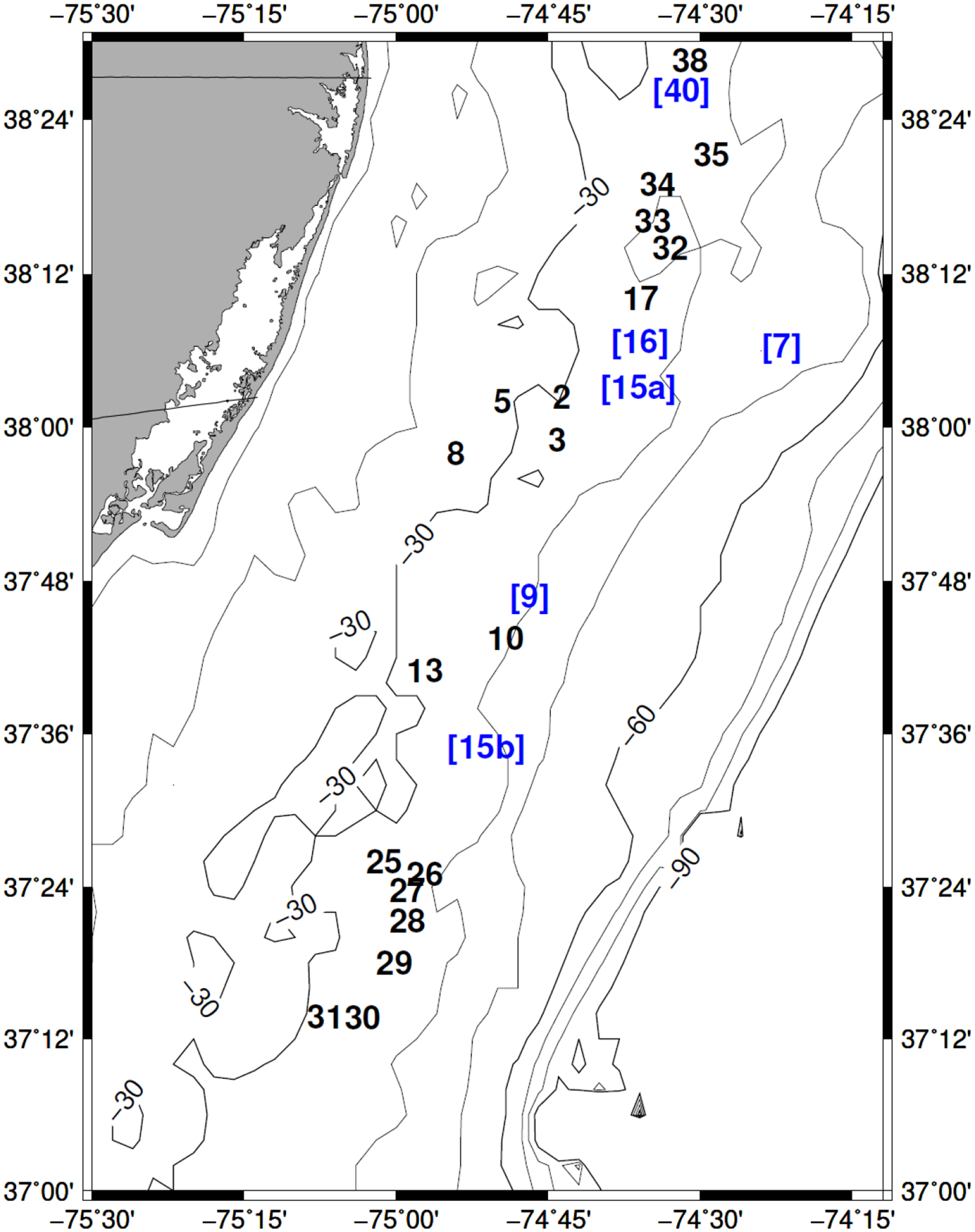
To investigate the timing of range shifts, dead ocean quahog shells were collected inshore of the species’ present-day southern inshore range boundary. A hydraulic dredge with a dredge width of 2.54 m was used to collect dead shells during an August 2019 research cruise aboard the F/V Betty C, a typical clam boat (Meyer et al., 1981; Parker, 1971). The dredge was lined with 1-inch square wire on the bottom and knife shelf, and 1 × 2-inch rectangular wire on the sides, back, and door. The wire lining retained clams ~⩾40 mm. Tows had a swept area of approximately 118 m² with tow distance limited to prevent overfilling of the dredge. Ocean quahogs shells were manually selected from the dredge haul material passed along a central belt. Sample stations extend along the continental shelf off the Delmarva Peninsula (Figure 1 and Table 1). Of the 27 stations sampled, 22 stations were also NEFSC federal survey stations for ocean quahogs and Atlantic surfclams sampled during 1982–2011 (NEFSC, 2017b) and identified by Powell et al. (2020). Five additional stations were added to this study from Powell et al. (2017).

Table 1.

Coordinates, depths, number of samples aged, and approximate birth dates of radiocarbon dated shells for stations shown in Figures 1 and 5 –7. Ages are calendar years from 2021.

Station number	Latitude (°N)	Longitude (°W)	Depth (M)	Radiocarbon ages (cal yr BP) (birth dates)	Climate events
2	38.0398	−74.7433	21.95	192, 207	Modern, Little Ice Age
3	37.9833	−74.7500	33.83	3427, 3452, 3462, 3467	Neoglacial
5	38.0333	−74.8450	24.99	237	Little Ice Age
7	38.1060	−74.3995	38.10	272, 2643, 2843, 2888, 3093, 3468, 3542, 3817	Little Ice Age, Neoglacial, Meghalayan Boundary
8	37.9666	−74.9166	23.77	61, 62, 62, 63	Modern
9	37.7652	−74.8140	34.44	243, 263,302, 2813, 3083, 3418, 4182	Little Ice Age, Neoglacial, Meghalayan Boundary
10	37.7258	−74.8507	31.70	3032, 3047, 3057	Neoglacial
13	37.6833	−74.9833	30.18	3472	Neoglacial
15a	38.0680	−74.6020	33.53	172, 177, 177, 177, 182, 182, 198, 262, 4302	Modern, Little Ice Age, Meghalayan Boundary
15b	37.5833	−74.9166	35.05	57, 132, 128, 158, 172, 212, 4392	Modern, Little Ice Age, Meghalayan Boundary
16	38.1127	−74.6000	33.83	137, 142, 157, 157, 177, 182, 182,182, 188, 193, 197, 198, 203, 212, 222, 3517, 4102	Modern, Little Ice Age, Neoglacial, Meghalayan Boundary
17	38.1525	−74.5986	39.93	167, 172, 177, 177	Modern
25	37.4333	−75.0500	28.04	157, 162, 167, 197, 2447	Modern, Roman Warm Period
26	37.4167	−74.9833	34.44	182, 858, 1168, 1183, 1187, 1187, 1187, 1188, 1208, 1212, 1223	Modern, Medieval Warm Period, Dark Ages
27	37.3950	−75.0117	33.53	72, 157, 162, 1167, 1207, 1223, 2578	Modern, Dark Ages, Neoglacial
28	37.3551	−75.0118	37.19	65, 197, 232, 242, 462	Modern, Little Ice Age
29	37.3000	−75.0333	36.88	177, 182, 197, 237	Modern, Little Ice Age
30	37.2285	−75.0858	32.00	2017, 3512, 3512, 3532	Roman Warm Period, Neoglacial
31	37.2299	−75.1469	29.57	162, 172, 187, 207, 877	Modern, Little Ice Age, Medieval Warm Period
32	38.2335	−74.5800	37.19	3437, 3447, 3472, 3502, 3527	Neoglacial
33	38.2685	−74.6090	39.32	212	Little Ice Age
34	38.3160	−74.6005	35.66	117, 137, 147	Modern
35	38.3537	−74.5118	33.22	157, 157, 192	Modern
38	38.4762	−74.5475	36.58	142, 202, 202	Modern
40	38.4378	−74.5790	32.61	4172, 4182	Meghalayan Boundary

Figure 1.

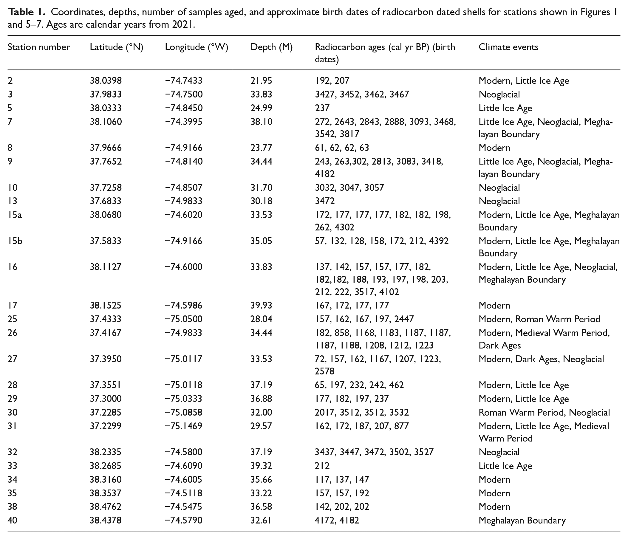
Map of sample stations as numbered during the survey. Bathymetric contour depths in meters. Bracket numbers in blue represent the station location where shells were dated during the first half of the Neoglacial period, approximately at the time of the Northgrippian-Meghalayan boundary of the Holocene. For a map of the present-day distribution of Arctica islandica, see Powell et al. (2020) and NEFSC (2017b).

Radiocarbon dating

Valves selected for dating were cut using a Kobalt wet tile saw. The valves were ground using 240 grit silicon carbide abrasive paper to remove any contaminants along the edge. Shell powder samples were extracted from half of the cut valve using a Dremel tool to grind the cut edge of the shell near the hinge and umbo to collect carbonate from the portion of the shell with early ontogenetic growth; that is, shell deposited during the first few years of life. Shell powder was collected and the resulting >10-mg sample was sent to the W. M. Keck Carbon Cycle Accelerator Mass Spectrometry Laboratory at the University of California, Irvine for analysis. Radiocarbon ages of samples will be referred to hereafter as birth years to clarify that the ages represent the time near the beginning of the lifespan which often exceeds 200 years for ocean quahogs.

Radiocarbon ages (±15–25 years depending on sample) were corrected for marine reservoir age (MRA) using Marine13 (400 years) (Reimer et al., 2013). MRA differs both temporally and spatially as a consequence of spatio-temporal variations in ocean mixing (Alves et al., 2018; Heaton et al., 2020). Ocean quahogs live in the Cold Pool, which derives water in varying proportions from Arctic and North Atlantic sources depending on the year (Chen and Curchitser, 2020; Chen et al., 2021; Miles et al., 2021; Wang et al., 2019), providing some uncertainty in this correction factor. In addition, the majority of earlier estimations for the North Atlantic come from the eastern Atlantic, greater depths, or higher latitudes, with mixes of water sources divergent from the composition of the Cold Pool (Ascough et al., 2007; Eiríksson et al., 2004; Heaton et al., 2020; Sherwood et al., 2008; Tisnérat-Laborde et al., 2010). Given the absence of a regional MRA in the MAB offshore of the Delmarva Peninsula, a series of live A. islandica were obtained from sites off New Jersey, Long Island, and Georges Bank as described by Hemeon et al. (2021) and Sower et al. (2022). Shells from live animals were processed and radiocarbon dated using the same method followed for dead shells.

A comparison of the birth year obtained by directly aging the shells of these live-caught bivalves to the radiocarbon ages obtained for their shells demonstrated a good fit to the Marine13 MRA correction factor of 400 years (Figure 2). The median residual when compared to the Marine13 MRA obtained from this comparison was 6.5 years, a mean of 7 years, and a standard deviation of ±40.47 years. Nevertheless, to constrain the potential error when calibrating marine carbon dates in this region, further research is needed to determine the regional variability in MRA in the Cold Pool. Given the presently available database shown in Figure 2, birth dates in this contribution were corrected under the assumption that bottom water conditions present at the time the dated shells were alive were consistent with the Marine13 MRA.

Figure 2.

Marine reservoir age residuals obtained by comparing the global marine reservoir age of 400 years from Marine13 (Reimer et al., 2013) with the birth dates determined by visual aging from a sample of live-caught radiocarbon-dated Arctica islandica obtained from Georges Bank (40.72767°N 67.79850°W, 72.5 m; Hemeon et al., 2021), Long Island (40.09658°N 73.01057 W, 47.5 m; Pace et al., 2017b), and northern New Jersey (39.33°N 73.12°W, 62.5 m).

Ocean quahogs alive after 1950 were exposed to bomb carbon from the detonation of the atomic bombs in the late 1950s and 1960s. Exposure to “bomb carbon” resulted in a spike of ¹⁴C in the shell. The reference time series of Δ¹⁴C (‰ deviation of the sample from the radiocarbon standard defined by Stuiver and Polach, 1977) determined by Kilada et al. (2007) was applied to radiocarbon values from ocean quahog shells to estimate birth years post-1950 (Scourse et al., 2012).

Results

A total of 121 Arctica islandica shells were radiocarbon-dated. Of these, 116 dead shells were born pre-bomb and 5 shells were born post-bomb. Radiocarbon ages ranged from 4392 to 61 cal BP (Table 1). Of the 121 shells dated, 60 were alive in the 1800–1900s (Figures 3 and 4). Most of these shells were alive between 1805 and 1865, within and just after the final years of the Little Ice Age (Cronin et al., 2010; Mann et al., 2009). Because of the uncertainty surrounding the exact end of the LIA, the ending of the LIA has been set arbitrarily to 1819 to split the radiocarbon dates obtained from this time period into two relatively equivalent groups. Radiocarbon dates for six more shells were between 4.3 and 4.1 cal ka BP, contemporaneous with the Northgrippian-Meghalayan boundary of the Holocene circa 4.2 cal ka BP (Figure 3a; Helama and Oinonen, 2019). Twenty-three A. islandica were born between 3.8 and 3.0 cal ka and 2.4 cal ka BP, coinciding with the time referred to as the Neoglacial Period (Figure 3a; Jennings et al., 2002; Larsen et al., 2012; Moossen et al., 2015; Wang et al., 2012). One dead shell lived in 2.0 cal ka BP which coincides with the Roman Warm Period (Wang et al., 2012). Twelve animals lived during the Dark Ages Cold Period (Figure 3b; Helama et al., 2017; Larsen et al., 2012; Moossen et al., 2015). Two shells were born in 0.8 cal ka BP toward the end of the Medieval Warm Period. The 18 shells recruited between 1500 and 1800 cal CE were alive during the Little Ice Age (Figure 3b; Cronin et al., 2019; Larsen et al., 2012).

Figure 3.

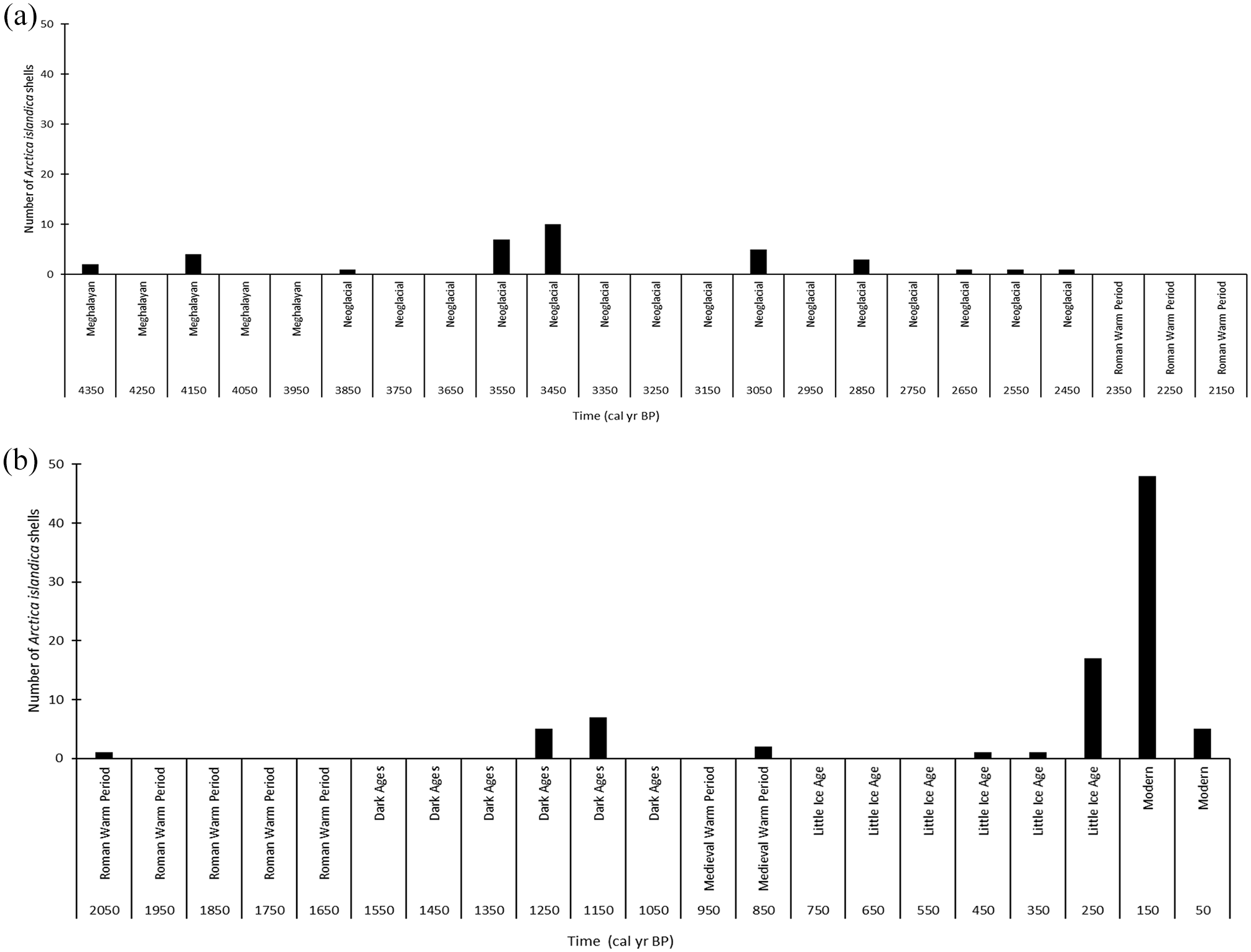
Panel (a) shows the frequency of Arctica islandica births in years before present (BP) and the simultaneous climate events: Northgrippian-Meghalayan Boundary (Helama and Oinonen, 2019). Neoglacial (Jennings et al., 2002), and Roman Warm Period (Moossen et al., 2015; Wang et al., 2012). Panel (b) shows the frequency of birthdates in years before present and the simultaneous climate events: Roman Warm Period (Moossen et al., 2015; Wang et al., 2012), Dark Ages Cold Period (Larsen et al., 2012), Medieval Warm Period (Graham et al., 2011), Little Ice Age (Ogilvie and Jónsson, 2001), and post-Little Ice Age (Modern).

Figure 4.

Shorter timeline focusing on the frequency of Arctica islandica birth years during the 19th century.

Shells collected from nine stations lived during the first half of the Neoglacial, around the 4.2 cal ka event (Figure 1). Two of the seven stations with shells dated during the Neoglacial also had shells dated during the 4.2 cal ka event (Figure 5). Shells at two collection sites were born during the Dark Ages Cold Period (Figure 6). Shells at 11 stations lived during the Little Ice Age, and shells at five of these stations also lived during previous cold periods (Figures 1 and 5). Shells at 15 stations lived between 1819 and 1965; at seven of these stations, shells lived during the Little Ice Age (Figure 7), and shells at three stations also lived during the Neoglacial periods (Figures 1, 5, and 7).

Figure 5.

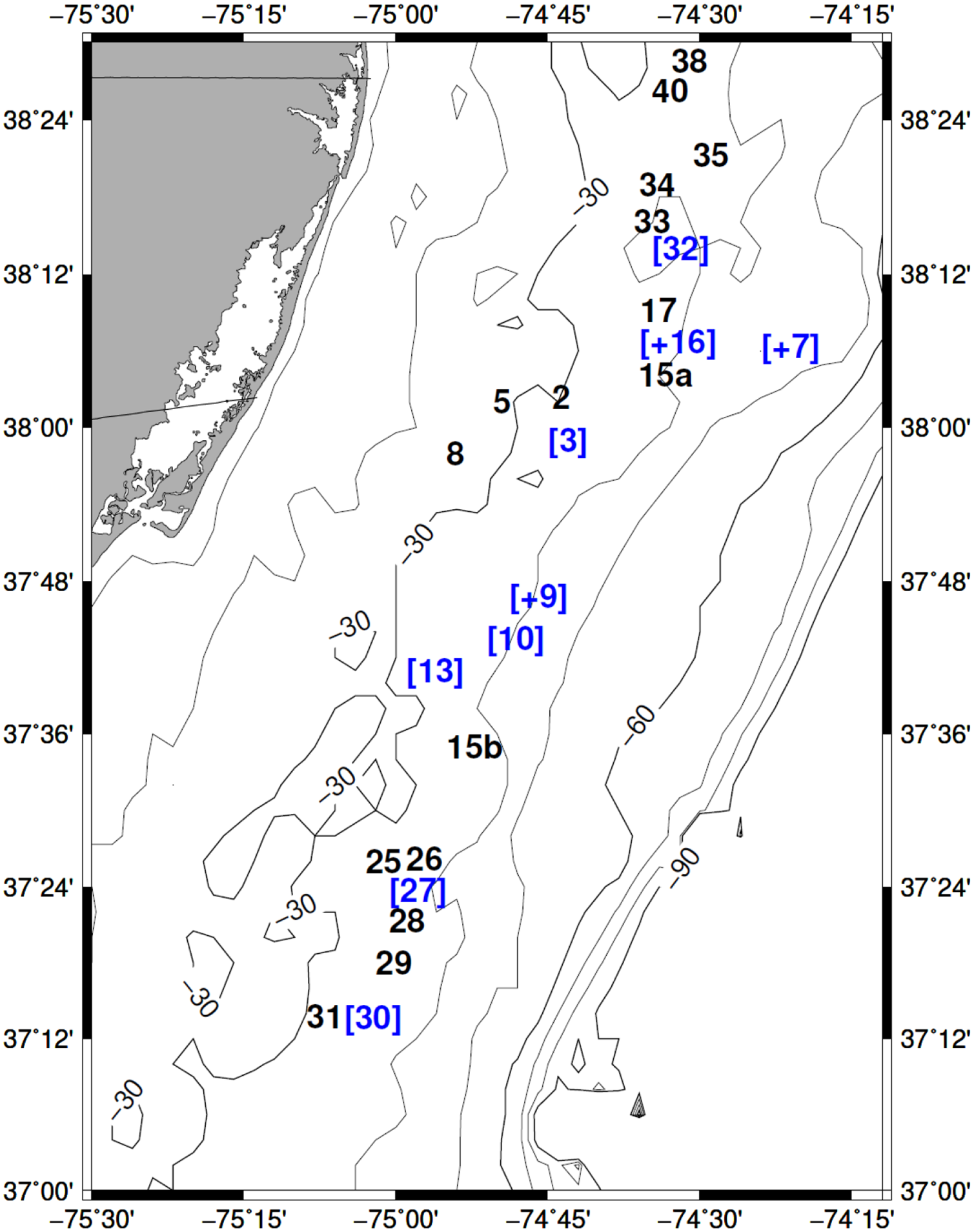
Map of sample stations as numbered during the survey. Bathymetric contour depths in meters. Bracket numbers in blue represent the station locations where shells were dated during the second half of the Neoglacial period. Station numbers with a plus represent stations with samples dated to multiple cold periods (Figure 1).

Figure 6.

Map of sample stations as numbered during the survey. Bathymetric contour depths in meters. Bracket numbers in blue represent the station locations where shells were dated during the Dark Ages Cold Period. Orange bracketed numbers represent shells dated during the Little Ice Age through 1819. Station numbers with a plus represent stations with samples dated to multiple cold periods (Figures 1 and 5).

Figure 7.

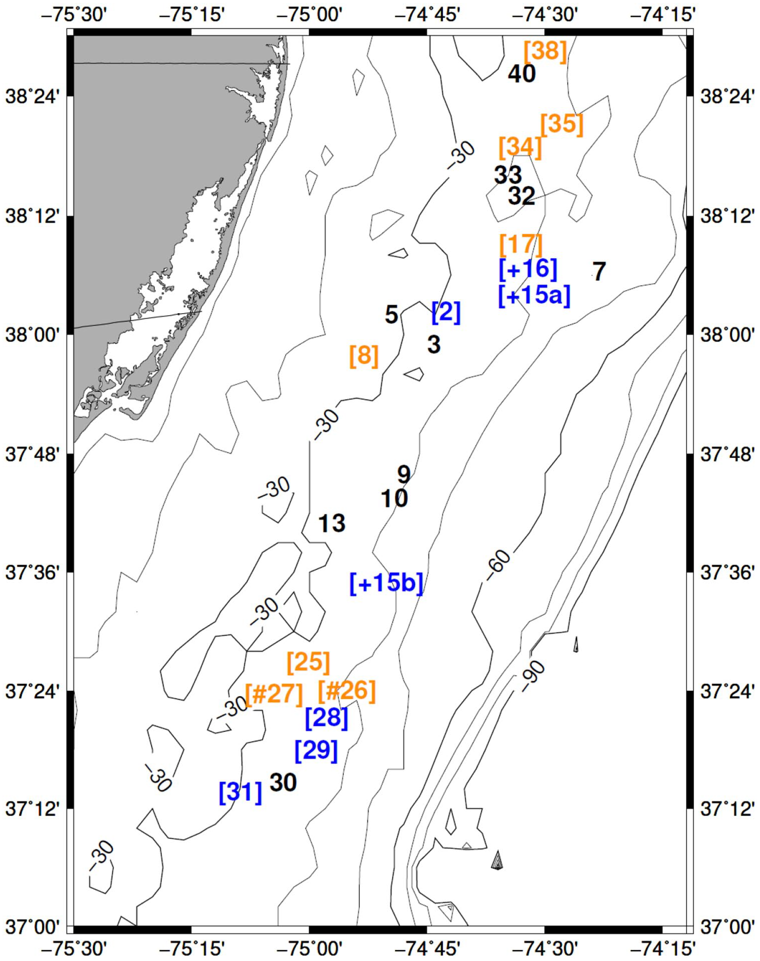
Map of sample stations as numbered during the survey. Bathymetric contour depths in meters. Bracketed numbers in blue represent stations where shells were dated during the Little Ice Age (Figure 6) and between 1819 and 1965. Station numbers with a plus show stations that yielded shells dating to the Neoglacial periods (Figures 1 and 5). Station numbers with a hashtag show stations that yielded shells dating to the Dark Ages Cold Period (Figure 6). Bracketed orange numbers show stations yielding shells that dated between 1819 and 1965, but not during the Little Ice Age.

The distribution of shell dates among stations showed that samples often included shells with dates from more than one previous cold period. Seven of 25 stations provided shells from more than one cold period, with three of these stations providing shells with dates from three cold periods. In addition, dead shells collected from nine stations were alive in 1820 or later and during the LIA (defined arbitrarily to end in 1819). Thus, the sampled stations were routinely occupied by ocean quahogs during earlier cold times and these multiply-occupied sites were also distributed throughout the sampled region.

Discussion

Understanding the death assemblage

Finding solely dead shells can indicate the spatial or temporal under-sampling of the community or allochthonous redistribution of shells (Kidwell, 2002; Staff and Powell, 1988). Although the possibility of allochthonous input cannot be ignored, the rarity of fishing vessel routes in the area suggests that ocean quahogs found offshore of Delmarva were not discarded shells from fishing vessels (e.g. NEFSC, 2017a, 2017b; see also Ropes, 1972, 1982). The geographic extent of the federal survey assures adequate sampling of the region and validates the absence of live animals at sampled stations and throughout the adjacent region. Moreover, the life span of the species minimizes the possibility of failing to capture live animals due to seasonal or interannual variations in abundance, a consideration for shorter-lived species (e.g. Kidwell, 2008; Staff and Powell, 1988, 1990). Finally, water depth limits any shoreward transport of shells by storms (Miles et al., 2015). The shells represent the remains of animals originally living at these sites and the birth years fall after the period of rapid sea-level rise in the early years of the Holocene, meaning that the MAB continental shelf depths were similar to today (Engelhart et al., 2011).

The number of the shells dated during a given time interval is not an indication of the relative abundance of the shells in situ, as no effort was made to age shells in proportion to the numbers retrieved by the dredge. The shells retrieved were present in the top ~8 cm of the sediment column, as hydraulic dredges are not designed to dig deep into the sediment. Only a small vertical section of the death assemblage was accessed; however, these dredges are efficient collectors of material in this surficial horizon (Poussard et al., 2021).

The time periods recorded by these shells in the death assemblage are a function of preservational processes, including limited burial rates, and shell degradation (Olszewski, 2004; Powell, 1992; Smith and Nelson, 2003; Tomasovych, 2004). Ocean quahogs shells degrade slowly and as a result persist in the death assemblage (Powell et al., 2008, 2011a, 2011b). Hence, age distributions observed support the inference that gaps in the distribution are likely to record times when living animals were not present, rather than a failure to be preserved. Large numbers of shells recorded from the 19th century relative to earlier times support the hypothesis of exponential loss in time-averaged assemblages proposed by Tomašových et al. (2014), Dexter et al. (2014), and Kosnik et al. (2009). Thus, the majority of birth dates being after 1800 CE does not indicate a lesser population abundance prior to those times.

Generality of findings

The distribution of birth dates among stations reveals that samples at the same station often included shells from more than one previous cold period. Stations were routinely occupied by ocean quahogs during multiple cold events and were distributed throughout the study region. Station samples containing shells from multiple climate events within the entire study region of approximately 1.5° of latitude suggests that the study does not include the entire geographic extent of past ocean quahog occupations, but rather suggests that further study would reveal a much more widespread occupation in the studied region for each of the cold periods identified.

Distribution and range shifts

The locations sampled harboring only dead clams are geographically distinct from the species present-day range (Figures 1 –4); therefore, the death assemblage preserves a record of past occupation and the historical shifting range of this species (Powell et al., 2020). Utilizing these data, the death assemblage in these areas can further the understanding of past, ongoing, and future range shifts consequent of changes in bottom water temperatures (Powell et al., 2020).

Sea bottom temperatures (SBTs) in the MAB directly affect the distribution of A. islandica (Dahlgren et al., 2000), as seen in the connection between the 16℃ isotherm and the inshore range of these boreal clams (Harding et al., 2008; Mann, 1982). Although A. islandica grow shell at temperatures as low as 0℃–1℃ ( Schöne et al., 2004; Wanamaker et al., 2008, 2011; Witbaard et al., 1998), in the MAB region, the minimum bottom temperature in the Cold Pool ranges between 4℃ and 5℃ (Chen and Curchitser, 2020) and the presence of clear growth increments confirms limited growth at these winter temperatures in MAB populations. Therefore, inferring a practical thermal range for adult ocean quahogs in the MAB to be between 4℃ and 16℃ (Harding et al., 2008), the presence of these shells suggests that bottom temperatures during their lifetimes were within the same thermal range (Powell et al., 2020). Currently, the SBTs in the sampled region (Figure 1) are too warm to support ocean quahogs and even too warm to continuously support Atlantic surfclams (Hofmann et al., 2018), which have a higher thermal maximum (Munroe et al., 2013; NEFSC, 2017a). During the late-Holocene, however, the distribution of A. islandica was both farther inshore and farther south than the present ocean quahog range (Figures 1 and 5 –7).

Shells containing radiocarbon from certain time periods indicate animals were alive when optimum environmental conditions prevailed for a boreal species. Over half of the radiocarbon dates indicate that animals were alive in the late 1700s to 1800s at these shallower inshore depths, years that are contemporaneous with the recruitment of the modern living population farther offshore in southern New Jersey (Pace et al., 2017b). This connection signifies that rising temperatures over the past 200 years are the likely cause of the disappearance of ocean quahogs from these inshore habitats. The remaining radiocarbon dates substantively predate the late 1700s–1800s. The majority of these years align with known cooling events in the late-Holocene (Mayewski et al., 2004; Wanner et al., 2011). Wanner et al. (2011) determined that the post-glacial climate was interrupted by six cold periods during the Holocene. Two periods occurred before the earliest birth of any sampled shells, indicating conditions were outside the optimal thermal range probably because lower sea level produced depths too shallow for habitation in the sampled region during these times. However, the other four cooling periods described by Wanner et al. (2011) correspond with A. islandica recovered from the MAB death assemblage. Negative temperature anomalies in North America reveal cooling events in 4.3–3.8, 3.3–2.5, 1.75–1.35, and 0.7–0.15 cal ka BP (Mayewski et al., 2004; Wanner et al., 2011). These times align with known past climate events including the Neoglacial, Dark Ages Cold Period, and Little Ice Age (Helama and Oinonen, 2019; Jennings et al., 2002; Larsen et al., 2012; Moossen et al., 2015; Wang et al., 2012) and are represented by ocean quahog shells dated in this study.

The exact timing and extent of the Neoglacial is uncertain, but estimates range between 6 and 2 cal ka BP (Jennings et al., 2002; Moossen et al., 2015; Weidick et al., 2012; Weiser et al., 2021). Shells dated between 4.4 and 3.8, 3.5–3.0, and 2.4 cal ka BP are contemporaneous with this time interval as well as specific cold events within it. The oldest shells coincide with the Northgrippian-Meghalayan boundary of the Holocene, an event marked by colder climate and a long megadrought that lasted from 4.2 to 3.9 cal ka BP as well as increased ice cap size in 4.2–3.0 cal ka BP (Helama and Oinonen, 2019; Larsen et al., 2012; Walker et al., 2018). Andersen et al. (2004) also inferred cooling events in 4.7, 4.3, and 2.8 cal ka BP from fossil diatoms found in the North Atlantic; these times align with the birth dates of the ocean quahogs.

Radiocarbon from one A. islandica sequestered during 2.0 cal ka BP, indicated a birth date within the RWP, the warming period that last from 2.3 to 1.6 cal ka BP. Despite evidence of a warming period in North America, during this time conditions were not above the temperature tolerance in the MAB for A. islandica at the sample station. Helama et al. (2017) reviewed the Dark Ages Cold Period (DACP) literature finding a more detailed chronology of DACP indicated an average start and end date of 450 and 800 cal CE, with a North Atlantic event of ice-rafted debris in the middle, about 1.4 cal ka BP, as well as support for a negative NAO phase. Additionally, another cooling phase within the DACP from 540 to 660 cal CE, identified as the “Late Antique Little Ice Age” (LALIA) can be seen within tree ring data (Büntgen et al., 2016; Helama et al., 2017). Six dead shells were alive at the end of these cooling events before the start of the MWP.

One shell collected was born at the tail end of the MWP and the start of the LIA and may indicate a prelude to the start of the LIA. Several shells date from the middle of the LIA, 462–222 cal BP. The majority of the radiocarbon dates in and after the LIA fall toward the end of the LIA in the early 19th century (Grove, 2004; Wanner et al., 2008), during the coldest portion of the LIA, and subsequently through the late 1800s cal CE. Sixteen dead shells had radiocarbon dates coinciding with this major cold event, indicating that the animals were alive in the 1840–1865 cal CE timeframe. Pace et al. (2017b) found an increase in ocean quahog recruitment before 1860 cal CE in a site just offshore and north of the region sampled in this study. Pace et al. (2017a) proposed that the increased recruitment may be related to the end of the LIA and the decline in shells with radiocarbon dates post-1865 cal CE might be interpreted as the initiation of increased mortality on the inshore edge of the range as temperatures continued to warm in the last half of the 19th century.

Although one cannot prove that the distribution of ages observed in this study is comprehensive of the time periods when ocean quahogs lived farther inshore than present-day, the near absence of shells born during the warm periods, RWP and MWP, strongly suggests that the distribution of birth dates observed identifies cold-period biogeographic range shifts inshore rather than the uncertain chance of collection. Powell et al. (2020) identified locations inshore and farther south of the present area of sampling from which were reported dead ocean quahog shells. Thus, this survey does not constrain either the inshore extent or southern extent of ocean quahog habitation during earlier cold times.

Conclusions

The death assemblage provides a view of the long-term geographic distributions of species prior to modern survey and monitoring programs. In particular, the death assemblage can provide a new view of the history of community response to climate change on the continental shelf over long time periods. In this study, shells of Arctica islandica were sampled on the Mid-Atlantic Bight (MAB) continental shelf at locations where living animals were not observed over the time of the 20th century federal survey time series. These shells identify habitable regions in the past that are not presently habitable by this species and in particular past times colder than today. Collection sites further inshore and south of the present range of the ocean quahog were once colder and thus suitable habitat for ocean quahogs. Looking at the aggregation of radiocarbon date frequencies, the inshore range of ocean quahogs has transgressed and regressed at least four times over the last 4500 years. The largest aggregation of radiocarbon dates reveals a recent ocean quahog transgression and regression inshore, with the regression likely beginning post-1865. Moreover, all of these dates coincide with historical times of cooling found in the Holocene climate literature. The radiocarbon dates obtained do not designate birth years randomly distributed over the time span of dated individuals. Very few shells date from times of warming, also well-documented in the Holocene climate literature, supporting the interpretation of range shifts onshore and offshore across the continental shelf as a consequence of climate warming and cooling phases with bottom water temperatures sufficient to permit and preclude the occupation of these long-lived bivalves.

The presence of these clams indicates that SBTs would need to be within the range of thermal tolerance for A. islandica, between ~5℃ and 15℃, during these cold phases. These comparisons can be used as predictive tools to determine future range shifts for ocean quahogs as climate change continues to increase bottom water temperatures in the MAB. The record provided by A. islandica may provide an important constraint on the modeling of the history of the Cold Pool which today determines the community structure of the continental shelf from Virginia to Georges Bank. Future work expanding the geographic footprint of dated A. islandica shells would be most valuable in this regard.

Footnotes

Acknowledgements

The authors would like to thank crew of the F/V Betty C for their assistance in collecting the samples and the use of their industry gear. The authors thank the National Marine Fisheries Service Northeast Fisheries Science Center (NEFSC) for making available the original datasets used in this study for site selection and we express particular appreciation of the efforts of the many individuals of the NEFSC survey branch that participated in survey data collection over the 1980–2011 time period that made this study possible.

Funding

The author(s) disclosed receipt of the following financial support for the research, authorship, and/or publication of this article: This research was supported by the National Science Foundation (NSF) through the Industry/University Cooperative Research Center (I/UCRC) program supporting the Science Center for Marine Fisheries (SCEMFIS) under NSF awards 1266057 and 1841112 and through membership fees provided by the SCEMFIS Industry Advisory Board. Conclusions and opinions expressed herein are solely those of the authors.

ORCID iD

Alyssa M LeClaire

References

Alves

Macario

Ascough

, et al. (2018) The worldwide marine radiocarbon reservoir effect: Definitions, mechanisms, and prospects. Reviews of Geophysics 56: 278–305.

Andersen

Koç

Moros

(2004) A highly unstable Holocene climate in the subpolar North Atlantic: Evidence from diatoms. Quaternary Science Reviews 23: 2155–2166.

Ascough

Cook

Dugmore

, et al. (2007) The North Atlantic marine reservoir effect in the Early Holocene: Implications for defining and understanding MRE values. Nuclear Instruments & Methods in Physics Research Section B, Beam Interactions with Materials and Atoms 259: 438–447.

Auger

Mayewski

Maasch

, et al. (2019) 2000 years of North Atlantic-Arctic climate. Quaternary Science Reviews 216: 1–17.

Bignami

Hopkins

(2003) Salt and heat trends in the shelf waters of the southern Middle-Atlantic Bight. Continental Shelf Research 23: 647–667.

Bizjack

Kidwell

Velarde

, et al. (2017) Detecting, sourcing, and age-dating dredged sediments on the open shelf, Southern California, using dead mollusk shells. Marine Pollution Bulletin 114: 448–465.

Büntgen

Myglan

Ljungqvist

, et al. (2016) Cooling and societal change during the late antique Little Ice Age from 536 to around 660 AD. Nature Geoscience 9: 231–236.

Butler

Wanamaker

Scourse

, et al. (2013) Variability of marine climate on the North Icelandic Shelf in a 1357-year proxy archive based on growth increments in the bivalve Arctica islandica. Palaeogeography Palaeoclimatology Palaeoecology 373: 141–151.

Castelao

Schofield

Glenn

, et al. (2008) Cross-shelf transport of freshwater on the New Jersey shelf. Journal of Geophysical Research Oceans 113: C07017.

10.

Chen

Tung

K-K

(2018) Global surface warming enhanced by weak Atlantic overturning circulation. Nature 559: 387–391.

11.

Chen

Curchitser

(2020) Interannual variability of the Mid-Atlantic Bight Cold Pool. Journal of Geophysical Research Oceans 125: e2020JCO016445.

12.

Chen

Kwon

Chen

, et al. (2021) Seasonal prediction of bottom temperature on the northeast U.S. continental shelf. Journal of Geophysical Research Oceans 126: e2021JC017187.

13.

Crippa

Azzarone

Bottini

, et al. (2019) Bio- and lithostratigraphy of lower Pleistocene marine successions in western Emilia (Italy) and their implications for the first occurrence of Arctica islandica in the Mediterranean Sea. Quaternary Research 92(2): 549–569.

14.

Cronin

Clevenger

Tibert

, et al. (2019) Holocene sea-level variability from Chesapeake Bay tidal marshes, USA. The Holocene 29: 1679–1693.

15.

Cronin

Hayo

Thunell

, et al. (2010) The medieval climate anomaly and Little Ice Age in Chesapeake Bay and the North Atlantic Ocean. Palaeogeography Palaeoclimatology Palaeoecology 297: 299–310.

16.

Dahlgren

Weinberg

Halanych

(2000) Phylogeography of the ocean quahog (Arctica islandica): Influences of paleoclimate on genetic diversity and species range. Marine Biology 137: 487–495.

17.

Dexter

Kaufman

Krause

, et al. (2014) A continuous multi-millennial record of surficial bivalve mollusk shells from the São Paulo Bight, Brazilian shelf. Quaternary Research 81: 274–283.

18.

Eiríksson

Larsen

Knudsen

, et al. (2004) Marine reservoir age variability and water mass distribution in the Iceland Sea. Quaternary Science Reviews 23: 2247–2268.

19.

Engelhart

Horton

Kemp

(2011) Holocene sea-level changes along the United States’ Atlantic Coast. Oceanography 24: 70–79.

20.

Fisher

JAD

Frank

Petrie

, et al. (2014) Life on the edge: environmental determinants of tilefish (Lopholatilus chamaeleonticeps) abundance since its virtual extinction in 1882. ICES Journal of Marine Science 71: 2371–2378.

21.

Friedland

Hare

(2007) Long-term trends and regime shifts in sea surface temperature on the continental shelf of the northeast United States. Continental Shelf Research 27: 2313–2328.

22.

Friedland

Morse

Manning

, et al. (2020) Trends and change points in surface and bottom thermal environments of the US northeast continental shelf ecosystem. Fisheries Oceanography 29: 396–414.

23.

Graham

Ammann

Fleitmann

, et al. (2011) Support for global climate reorganization during the “Medieval Climate Anomaly”. Climate Dynamics 37: 1217–1245.

24.

Grove

(2004) Little Ice Ages: Ancient and Modern. New York, NY: Routledge.

25.

Hanna

Jónsson

Box

(2004) An analysis of Icelandic climate since the nineteenth century. International Journal of Climatology 24: 1193–1210.

26.

Harding

King

Powell

, et al. (2008) Decadal trends in age structure and recruitment patterns of ocean quahogs Arctica islandica from the mid-Atlantic Bight in relation to water temperature. Journal of Shellfish Research 27: 667–690.

27.

Heaton

Köhler

Butzin

, et al. (2020) Marine20—The marine radiocarbon age calibration curve (0–55,000 cal BP). Radiocarbon 62: 779–820.

28.

Helama

Jones

Briffa

(2017) Dark Ages Cold Period: A literature review and directions for future research. The Holocene 27: 1600–1606.

29.

Helama

Oinonen

(2019) Exact dating of the Meghalayan lower boundary based on high-latitude tree-ring isotope chronology. Quaternary Science Reviews 214: 178–184.

30.

Hemeon

Powell

Pace

, et al. (2021) Population dynamics of Arctica islandica at Georges Bank (USA): An analysis of sex-based demographics. Journal of the Marine Biological Association of the United Kingdom 101: 1003–1018.

31.

Hennen

(2015) How should we harvest an animal that can live for centuries? North American Journal of Fisheries Management 35: 512–527.

32.

Hofmann

Powell

Klinck

, et al. (2018) An overview of factors affecting distribution of the Atlantic surfclam (Spisula solidissima), a continental shelf biomass dominant, during a period of climate change. Journal of Shellfish Research 37: 821–831.

33.

Holland

Schöne

Lipowski

, et al. (2014) Decadal climate variability of the North Sea during the last millennium reconstructed from bivalve shells (Arctica islandica). The Holocene 24: 771–786.

34.

Hou

Halfar

Adey

, et al. (2019) Long-lived coralline alga records multidecadal variability in Labrador Sea carbon isotopes. Chemical Geology 526: 93–100.

35.

Houghton

Schlitz

Beardsley

, et al. (1982) The Middle Atlantic Bight Cold Pool: Evolution of the temperature structure during summer 1979. Journal of Physical Oceanography 12: 1019–1029.

36.

Hulme

Jones

(1994) Global climate change in the instrumental period. Environmental Pollution 83: 23–36.

37.

Jennings

Knudsen

Hald

, et al. (2002) A mid-Holocene shift in Arctic sea-ice variability on the East Greenland Shelf. The Holocene 12: 49–58.

38.

Kang

Curchitser

(2013) Gulf Stream eddy characteristics in a high-resolution ocean model. Journal of Geophysical Research Oceans 118: 4474–4487.

39.

Kavanaugh

Rheuban

Luis

KMA

, et al. (2017) Thirty-three years of ocean benthic warming along the U.S. northeast continental shelf and slope: Patterns, drivers, and ecological consequences. Journal of Geophysical Research Oceans 122: 9399–9414.

40.

Kidwell

(2002) Time-averaged molluscan death assemblages: Palimpsests of richness, snapshots of abundance. Geology 30: 803–806.

41.

Kidwell

(2007) Discordance between living and death assemblages as evidence for anthropogenic ecological change. Proceedings of the National Academy of Sciences of the United States of America 104: 17701–17706.

42.

Kidwell

(2008) Ecological fidelity of open marine molluscan death assemblages: Effects of post-mortem transportation, shelf health, and taphonomic inertia. Lethaia 41: 199–217.

43.

Kilada

Campana

Roddick

(2007) Validated age, growth, and mortality estimates of the ocean quahog (Arctica islandica) in the western Atlantic. ICES Journal of Marine Science 64: 31–38.

44.

Kosnik

Hua

Kaufman

, et al. (2009) Taphonomic bias and time-averaging in tropical molluscan death assemblages: Differential shell half-lives in Great Barrier Reef sediment. Paleobiology 35: 565–586.

45.

Larsen

Miller

Geirsdóttir , et al. (2012) Non-linear Holocene climate evolution in the North Atlantic: A high-resolution, multi-proxy record of glacier activity and environmental change from Hvítárvatn, central Iceland. Quaternary Science Reviews 39: 14–25.

46.

Lentz

(2017) Seasonal warming of the Middle Atlantic Bight Cold Pool. Journal of Geophysical Research Oceans 122: 941–954.

47.

Lucey

Nye

(2010) Shifting species assemblages in the northeast US continental shelf large marine ecosystem. Marine Ecology Progress Series 415: 23–33.

48.

Mann

Zhang

Rutherford

, et al. (2009) Global signatures and dynamical origins of the Little Ice Age and medieval climate anomaly. Science 326: 1256–1260.

49.

Mann

(1982) The seasonal cycle of gonadal development in Arctica islandica from the southern New England shelf. Fishery Bulletin 80: 315–326.

50.

Mayewski

Rohling

Stager

, et al. (2004) Holocene climate variability. Quaternary Research 62: 243–255.

51.

Meadows

Grebmeier

Kidwell

(2019) High-latitude benthic bivalve biomass and recent climate change: Testing the power of live-dead discordance in the Pacific Arctic. Deep-Sea Research Part II, Topical Studies in Oceanography 162: 152–163.

52.

Merrill

Ropes

(1969) The general distribution of the surf clam and ocean quahog. Proceedings of the National Shellfisheries Association 59: 40–45.

53.

Mette

Wanamaker

Jr Carroll

, et al. (2016) Linking large-scale climate variability with Arctica islandica shell growth and geochemistry in northern Norway. Limnology and Oceanography 61: 748–764.

54.

Meyer

Cooper

Pecci

(1981) The performance and environmental effects of a hydraulic clam dredge. Marine Fisheries Review 43(9): 14–22.

55.

Miles

Murphy

Kohut

, et al. (2021) Offshore wind energy and the Mid-Atlantic Cold Pool: A review of potential interactions. Marine Technology Society Journal 55: 72–87.

56.

Miles

Seroka

Kohut

, et al. (2015) Glider observations and modeling of sediment transport in Hurricane sandy. Journal of Geophysical Research Oceans 120: 1771–1791.

57.

Moore

GWK

Halfar

Majeed

, et al. (2017) Amplification of the Atlantic multidecadal oscillation associated with the onset of the industrial-era warming. Science Reports 7: 40861.

58.

Moossen

Bendle

Seki

, et al. (2015) North Atlantic Holocene climate evolution recorded by high-resolution terrestrial and marine biomarker records. Quaternary Science Reviews 129: 111–127.

59.

Munroe

Powell

Mann

, et al. (2013) Underestimation of primary productivity on continental shelves: Evidence from maximum size of extant surfclam (Spisula solidissima) populations. Fisheries Oceanography 22: 220–233.

60.

NEFSC (2017a) 61st Northeast Regional Stock Assessment Workshop (61st SAW) assessment report. US Department of Commercial Northeast Fisheries Science Center Reference Documents 17-05: 466.

61.

NEFSC (2017b) 63rd Northeast Regional Stock Assessment Workshop (63rd SAW) assessment report. US Department of Commercial Northeast Fisheries Science Center Reference Documents 17-10: 822.

62.

Negri

Sanfilippo

Basso

, et al. (2015) Comparison of live and dead molluscan assemblages suggests recent human-driven decline in benthic diversity in Phetchaburi (NW Gulf of Thailand). Continental Shelf Research 111: 9–30.

63.

Neto

Langan

Palter

(2021) Changes in the Gulf Stream preceded rapid warming of the Northwest Atlantic shelf. Communications Earth & Environment 2: 74.

64.

Ogilvie

Jónsson

(2001) “Little Ice Age” research: A perspective from Iceland. Climatic Change 48: 9–52.

65.

Olszewski

(2004) Modeling the influence of taphonomic destruction, reworking, and burial on time-averaging in fossil accumulations. Palaios 19: 39–50.

66.

Pace

Powell

Mann

, et al. (2017a) Development of an age—Frequency distribution for ocean quahogs (Arctica islandica) on Georges Bank. Journal of Shellfish Research 36: 41–53.

67.

Pace

Powell

Mann

, et al. (2017b) Comparison of age-frequency distributions for ocean quahogs (Arctica islandica) on the western Atlantic US continental shelf. Marine Ecology Progress Series 585: 81–98.

68.

Pace

Powell

Mann

(2018) Two-hundred year record of increasing growth rates for ocean quahogs (Arctica islandica) from the northwestern Atlantic Ocean. Journal of Experimental Marine Biology and Ecology 503: 8–22.

69.

Parker

(1971) History and development of surf clam harvesting gear (Vol. 364) US Department of Commerce, National Marine Fisheries Service, National Oceanic and Atmospheric Administration.

70.

Pershing

Alexander

Hernandez

, et al. (2015) Slow adaptation in the face of rapid warming leads to collapse of the Gulf of Maine cod fishery. Science 350: 809–812.

71.

Poussard

Powell

Hennen

(2021) Discriminating between high- and low-quality field depletion experiments through simulation analysis. Fishery Bulletin 119(4): 27–293.

72.

Powell

(1992) A model for death assemblage formation. Can sediment shelliness be explained? Journal of Marine Research 50: 229–265.

73.

Powell

Staff

Callender

, et al. (2011a) Taphonomic degradation of molluscan remains during thirteen years on the continental shelf and slope of the northwestern Gulf of Mexico. Palaeogeography Palaeoclimatology Palaeoecology 312: 209–232.

74.

Powell

Staff

Callender

, et al. (2011b) The influence of molluscan taxon on taphofacies development over a broad range of environments of preservation: The SSETI experience. Palaeogeography Palaeoclimatology Palaeoecology 312: 233–264.

75.

Powell

Callender

Staff

, et al. (2008) Mollusc shell condition after eight years on the sea floor — Taphonomy in the Gulf of Mexico and Bahamas. Journal of Shellfish Research 27: 191–225.

76.

Powell

Ewing

Kuykendall

(2020) Ocean quahogs (Arctica islandica) and Atlantic surfclams (Spisula solidissima) on the mid-Atlantic Bight continental shelf and Georges Bank: The death assemblage as a recorder of climate change and the reorganization of the continental shelf benthos. Palaeogeography Palaeoclimatology Palaeoecology 537: 109205.

77.

Powell

Mann

Ashton-Alcox

, et al. (2017) Can we estimate molluscan abundance and biomass on the continental shelf? Estuarine, Coastal and Shelf Science 198: 213–224.

78.

Reimer

Bard

Bayliss

, et al. (2013) IntCal13 and Marine13 radiocarbon age calibration curves 0–50,000 years cal BP. Turnery CSM and van der Plicht J 55: 1869–1887.

79.

Reynolds

Richardson

Scourse

, et al. (2017) Reconstructing North Atlantic marine climate variability using an absolutely-dated sclerochronological network. Palaeogeography Palaeoclimatology Palaeoecology 465: 333–346.

80.

Reynolds

Scourse

Halloran

, et al. (2016) Annually resolved North Atlantic marine climate over the last millennium. Nature Communications 7: 13502.

81.

Ropes

(1972) The Atlantic coast surf clam fishery 1965–1969. Marine Fisheries Review 34(7–8): 20–29.

82.

Ropes

(1982) The Atlantic coast surf clam fishery, 1965–1974. Marine Fisheries Review 44(8): 1–14.

83.

Saba

Griffies

Anderson

, et al. (2016) Enhanced warming of the northwest Atlantic Ocean under climate change. Journal of Geophysical Research Oceans 121: 118–132.

84.

Sachs

(2007) Cooling of northwest Atlantic slope waters during the Holocene. Geophysical Research Letters 34(3): L03609.

85.

Scavia

Field

Boesch

, et al. (2002) Climate change impacts on U.S. coastal and marine ecosystems. Estuaries 25: 149–164.

86.

Schöne

Freyre Castro

Fiebig

, et al. (2004) Sea surface water temperatures over the period 1884–1983 reconstructed from oxygen isotope ratios of a bivalve mollusk shell (Arctica islandica, southern North Sea). Palaeogeography Palaeoclimatology Palaeoecology 212: 215–232.

87.

Schöne

Pfeiffer

Pohlmann

, et al. (2005) A seasonally resolved bottom-water temperature record for the period AD 1866–2002 based on shells of Arctica islandica (Mollusca; North Sea). International Journal of Climatology 25: 947–962.

88.

Scourse

Wanamaker

Weidman

, et al. (2012) The marine radiocarbon bomb pulse across the temperate North Atlantic: A compilation of Δ¹⁴C time histories from Arctica islandica growth increments. Radiocarbon 54(2): 165–186.

89.

Sherwood

Edinger

Guilderson

, et al. (2008) Late Holocene radiocarbon variability in northwest Atlantic slope waters. Earth and Planetary Science Letters 275: 146–153.

90.

Smith

Nelson

(2003) Effects of early sea-floor processes on the taphonomy o temperate shelf skeletal carbonate deposits. Earth-Science Reviews 63: 1–31.

91.

Sower

Powell

Mann

, et al. (2022) New Jersey Ocean Quahog Population Dynamics [Unpublished manuscript].

92.

Staff

Powell

(1988) The paleoecological significance of diversity: The effect of time averaging and differential preservation on macroinvertebrate species richness in death assemblages. Palaeogeography Palaeoclimatology Palaeoecology 63: 73–89.

93.

Staff

Powell

(1990) Local variability of taphonomic attributes in a parautochthonous assemblage: Can taphonomic signature distinguish a heterogeneous environment? Journal of Paleontology 64: 648–658.

94.

Stuiver

Polach

(1977) Discussion reporting of ¹⁴C data. Radiocarbon 19: 355–363.

95.

Tisnérat-Laborde

Paterne

Métivier

, et al. (2010) Variability of the northeast Atlantic sea surface Δ¹⁴C and marine reservoir age and the North Atlantic Oscillation (NAO). Quaternary Science Reviews 29: 2633–2646.

96.

Tomasovych

(2004) Postmortem durability and population dynamics affecting the fidelity of brachiopod size-frequency distributions. Palaios 19: 477–496.

97.

Tomašových

Kidwell

Barber

, et al. (2014) Long-term accumulation of carbonate shells reflects a 100-fold drop in loss rate. Geology 42: 819–822.

98.

von Leesen

Beierlein

Scarponi

, et al. (2017) A low seasonality scenario in the Mediterranean Sea during the Calabrian (Early Pleistocene) inferred from fossil Arctica islandica shells. Palaeogeography Palaeoclimatology Palaeoecology 485: 706–714.

99.

Walker

Gibbard

Head

, et al. (2018) Formal subdivision of the Holocene Series/Epoch: A summary. Journal of the Geological Society of India 93: 135–141.

100.

Wallace

Looney

Gong

(2018) Multi-decadal trends and variability in temperature and salinity in the Mid-Atlantic Bight, Georges Bank, and Gulf of Maine. Journal of Marine Research 76: 163–215.

101.

Wanamaker

Jr Kreutz

Schöne

, et al. (2008) Coupled North Atlantic slope water forcing on Gulf of Maine temperatures over the past millennium. Climate Dynamics 31: 183–194.

102.

Wanamaker

Jr Kreutz

Schöne

, et al. (2011) Gulf of Maine shells reveal changes in seawater temperature seasonality during the medieval climate anomaly and the Little Ice Age. Palaeogeography Palaeoclimatology Palaeoecology 302: 47–51.

103.

Wang

Surge

Mithen

(2012) Seasonal temperature variability of the neoglacial (3300–2500 BP) and Roman warm period (2500–1600 BP) reconstructed from oxygen isotope ratios of limpet shells (Patella vulgata), Northwest Scotland. Palaeogeography Palaeoclimatology Palaeoecology 317: 104–113.

104.

Wang

Brickman

Greenan

BJW

(2019) Characteristic evolution of the Atlantic Meridional Overturning Circulation from 1990 to 2015: An eddy-resolving ocean model study. Deep Sea Research Part I Oceanographic Research Papers 149: 103056.

105.

Wanner

Beer

Bütikofer

, et al. (2008) Mid-to Late-Holocene climate change: An overview. Quaternary Science Reviews 27(19–20): 1791–1828.

106.

Wanner

Solomina

Grosjean

, et al. (2011) Structure and origin of Holocene cold events. Quaternary Science Reviews 30: 3109–3123.

107.

Weidick

Bennike

Citterio

, et al. (2012) Neoglacial and historical glacier changes around Kangersuneq fjord in southern West Greenland. GEUS Bulletin 27: 1–68.

108.

Weidman

Jones

Lohmann

(1994) The long-lived mollusc Arctica islandica: A new paleoceanographic tool for the reconstruction of bottom temperatures for the continental shelves of the northern North Atlantic Ocean. Journal of Geophysical Research C Oceans 99: 18305–18314.

109.

Weinberg

(2005) Bathymetric shift in the distribution of Atlantic surfclams: Response to warmer ocean temperatures. ICES Journal of Marine Science 62: 1444–1453.

110.

Weiser

Titschack

Kienast

, et al. (2021) Atlantic water inflow to Labrador Sea and its interaction with ice sheet dynamics during the Holocene. Quaternary Science Reviews 256: 106833.

111.

Witbaard

Franken

Visser

(1998) Growth of juvenile Arctica islandica under experimental conditions. Helgoländer Meeresuntersuchngen 51: 417–431.