Isolation basin stratigraphy and Holocene relative sea-level change on the Barents Sea coast at Teriberka,Kola Peninsula,northwestern Russia

Abstract

The paper presents isolation basin stratigraphy in bottom sediments from nine lakes in the Teriberka area on the Kola Peninsula, northwestern Russia. Isolation contacts in these basins, identified from lithological and diatom analysis, were used together with 25 radiocarbon dates, to construct a relative sea-level (RSL) curve for the Holocene. Records of marine water re-influx were found in the sediment sequence from one lake, located at c. 17 m a.s.l. The re-influx of marine water seems to be caused by the mid-Holocene (Tapes) transgression and tsunami event. The RSL curve indicates several phases in the postglacial evolution of the Kola coast. An early phase of rapid sea-level fall of c. 32 m around 11,500 cal yr BP, at a rate of c. 40 mm per year, corresponds to glacio-isostatically induced emergence following deglaciation at the Younger Dryas and beginning of the Holocene. In the time interval between c. 11,000 and 7600 cal yr BP, either a stillstand or a slight rise in relative sea level, cresting at about 21 m a.s.l., is suggested in the Teriberka area. This is followed, after c. 7300 cal yr BP to the present day, by a slow glacioisostatic emergence with an average rate of about 2–3 mm per year.

Keywords

diatoms glacio-isostasy Holocene Kola Peninsula lake sediments radiocarbon age sea-level changes Storegga tsunami

Introduction

Located at the margin of the Late Valdaian (Late Weichselian) Fennoscandian Ice Sheet on the Murmansk coast of the Kola Peninsula, small lakes (Figure 1), isolated from the sea during emergence, provide evidence of sea-level change during the Holocene. This setting is important for estimation of the sea-level changes to be used in glacio-isostatic geophysical modelling (Lambeck et al., 1998) and for studying isostatic crustal uplift resulting from deglaciation of the Kola Peninsula and adjacent sea shelf. Holocene relative sea level (RSL) changes on the Barents Sea coast have been studied since the late 19th century. Ramsay (1898, 1924) was the first to reconstruct the tectonic uplift and marine shoreline displacements, reasoning from the location of coastal landforms on the Kola Peninsula. When interpreting these displacements, he followed the ideas of de Geer (1890) and Högbom (1913) about the dome-shaped glacio-isostatic uplift of the Fennoscandian Shield, with maximum uplift occurring at the head of the Bothnian Gulf. In the early 20th century, V. Tanner (1930, 1936) identified the marine limit, as well as other shorelines, on the western Murmansk coast by plotting the altitudes of marine terraces identified in the river valleys. Tanner’s research initiated the systematic study of coastal landforms in Finnmark and the Kola Peninsula. In the 1940s-70s, Goretskiy (1941), Lavrova (1960), Nikonov (1964), and Koshechkin (1979) studied coastal landforms, marine shoreline displacements and tectonics on the western Murmansk coast, using mainly geomorphic profiles and shoreline isobase mapping. These studies were hampered by limited age control; shorelines can rarely be dated directly and available¹⁴C dates were mostly derived from mollusc shells or based on archaeological artefacts, which provide only maximum and minimum ages for corresponding RSL. Various models of glacio-isostatic uplift were constructed based on these data, but they differ considerably from each other due to the poor initial data.

Figure 1.

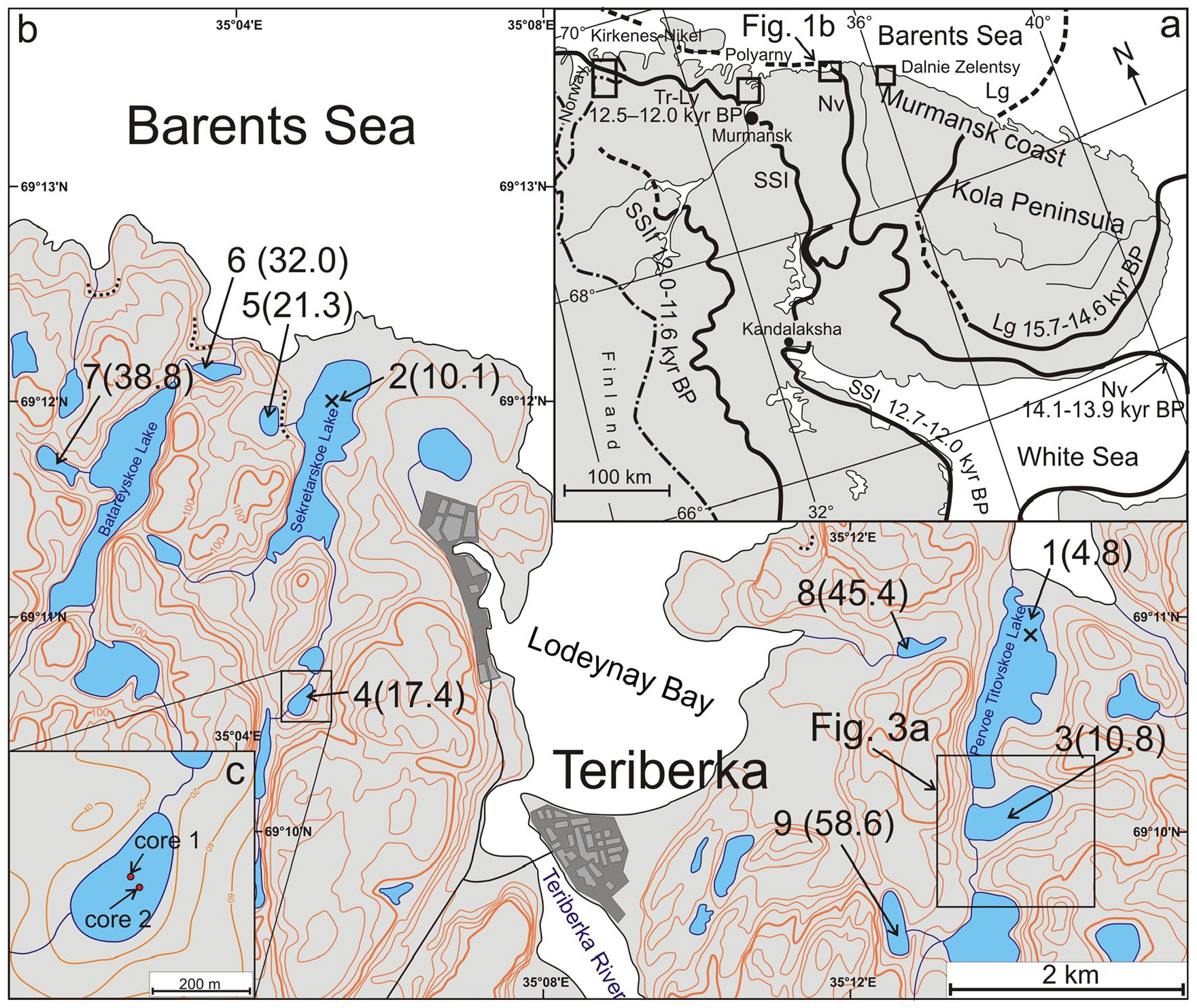
Location map showing. (a) The eastern flank of the Fennoscandian Ice Sheet during deglaciation and the location of studied areas (rectangles). Ice marginal positions at different stages (thick lines) are according to Korsakova et al. (2023a, 2023b) (Abbreviations show the stades: Lg–Luga (15.7–14.6 cal kyr BP), Nv–Neva (14.1–13.9 cal kyr BP), SSI –Salpausselkä I (c. 12.7–12.0 cal kyr BP) and Tr-Ly–Tromsø-Lyngen in the northeast of the region (c. 12.5–12.0 cal kyr BP, after Vorren and Plassen (2002)), SSII – Salpausselkä II (c. 12.0–11.6 cal kyr BP). (b) Location of the cored lake basins 1–9 in the Teriberka area, the elevation of lake threshold is indicated in brackets; a crosses indicate the coring sites in the largest lakes; topography is shown by a 20 m contour interval; the location of coastal landforms at an elevation of 20–22 m is shown by dotted lines. (c) Core sampling sites (red dots) in the lake 4 basin.

Reliable data on the sea coastline changes appeared from the mid-20th century using the isolation basins method (Donner et al., 1977; Hafsten, 1960). RSL curves were constructed for the western Murmansk Сoast in Russia (Corner et al., 1999, 2001; Snyder et al., 2008a) and for the coast of Finnmark in northern Norway (Romundset et al., 2011). These study areas are variously located in relation to the marginal moraines of the Fennoscandian Ice Sheet on the westernmost Murmansk coast (Figure 1a). The Kirkenes– Nikel area (Corner et al., 1999) is located 5–20 km inside the Younger Dryas Tromso-Lyngen end moraine (Figure 1a). The Polyarny area (Corner et al., 2001) is located close to the Younger Dryas Salpausselka I (cf. Korsakova et al., 2023b) end moraine zone, on the western side of the Kola fjord, 120 km east of the Kirkenes–Nikel area. The Dalnie Zelentsy area is located between the Luga (Keiva I) and Neva (Keiva II) marginal moraine zones (Korsakova et al., 2023a). The RSL curves from these areas illustrate different isostatic response to glacial unloading on the western Murmansk coast, related to their position in relation to the retreating ice margin.

This paper presents the results of a study of postglacial RSL change in the Teriberka area, which is located immediately inside the Neva (Keiva II) end moraine zone, midway between Polyarny and Dalnie Zelentsy (Figure 1a and b). The new data, based on the lithology and diatoms of lake sediments and radiocarbon dating of the timing of lake isolation, provide information on the age of deglaciation in the study area and give a more complete record of postglacial RSL change on the Murmansk coast.

Previous work in the Teriberka area, identified sediments of one lake (lake 4 in Figure 1b) thought to have been inundated during the Tapes transgression. The succession includes a layer of disturbed sediments, interpreted as having formed as a result of a catastrophic event (Nikolaeva et al., 2019; Tolstobrov et al., 2018). Additional work to study the sediments of this lake has been carried out and the results are presented in this article.

Study area

The study area is located near the Teriberka settlement (N 69°12′; E 035°05′), around Teriberka Bay on the Barents Sea coast, 80 km east of Murmansk (Figure 1). The bedrock is part of the Fennoscandian (Baltic) Shield and comprises igneous leucogranite and granodiorite of the Archaean Teriberka complex (Mitrofanov, 1996). The lakes occupy glacially eroded rock basins in an area of undulating, highly dissected relief, comprising small hills and plateaus reaching up to 190 m a.s.l. Glacial deposits, including gravelly and sandy till, and glaciofluvial ice-margin deposits and outwash, occur locally in interstream areas and depressions (Niemelä et al., 1993). Striae, drumlins, eskers and end moraines on the Murmansk coast indicate a dominant north-northeasterly ice-sheet flow from the central Kola Peninsula (e.g. Niemelä et al., 1993; Stroeven et al., 2016). Late Glacial and Holocene marine sediments occur locally in open coastal areas (Koshechkin 1979).

Tundra vegetation, dominated by sedges, diverse tundra herbs, and mosses occurs at poorly drained sites, accompanied by scattered birch stands at low elevations and in protected areas. The present forest limit lies about 10 km south of the study area (Kremenetski et al., 2008). Tidal range, according to data from nearest tide station on the Teriberka Bay coast, is approximately 4.0–4.3 m (Terziev et al., 1990). Near the Teriberka settlement, mean temperature in January and July is −8.4°C and 10.7°C, respectively and mean annual precipitation is 600 mm (Kalabin, 1999).

The studied lakes are located in a small area of 8 km×4 km. Lake basins range in size from 0.03 to 0.70 km² and their maximum water depth is between 2 and >15 m. Drainage into the lakes is by seepage or from small streams.

The marine limit at Teriberka area has not been established. In the Kirkenes–Nickel, Polyarny and Dalnie Zelentsy areas, the marine limit has been located at 90, 80, and 60 m a.s.l., respectively. Coastal landforms have been identified previously in the Teriberka area up to c. 60 m a.s.l., among them the mid-Holocene, Tapes transgression-maximum shoreline (beach ridge) which is located at an elevation of 20–25 m a.s.l. (Koshechkin 1979; Snyder et al., 2008b). The Tapes shoreline was found at an elevation of about 20–22 m a.s.l. at one of the investigated lakes (lake 5 in Figure 1b) at Teriberka.

Methods

We applied the so-called isolation basins method (Hafsten, 1960; Kjemperud, 2008) to reconstruct RSL changes. The method is widely used in areas experiencing glacio-isostatic adjustment after the retreat last ice sheet (Corner et al., 1999, 2001; Kolka et al., 2013; Romundset et al., 2011; Snyder et al., 2008a). Isolation basin develops when RSL fall causes marine inlet to become disconnected from the sea, forming, first, a brackish lagoon, which then becomes a freshwater lake. Recognizing the isolation contact in the sediment column using lithological and biostratigraphic indicators and ¹⁴C dating of the corresponding sediments, allows the elevation of the lake threshold at the time of isolation to be identified and dated. Data from several lakes located at different elevations allow construction of a RSL curve.

Field work

Sediment cores were taken from ice-covered lakes in April, 2013, 2016, and 2018, using a portable piston corer with 54 mm diameter. Bathymetric measurements were provided using a portable echosounder to recognize the location with flat bottom for core sampling. We pushed the equipment as far as we could, normally down to bedrock or glacial till. Cores were taken in 1 m lengths with a 10 cm overlap to obtain a complete sedimentary sequence. Correlation of the cores was made by matching layers or horizons together with their measured depth below the lake surface. Lithological description and sampling for diatom analysis and radiocarbon dating were done in the field. Sediments slices were collected for diatom analysis (1–2 cm thick) and radiocarbon dating (5–10 cm thick).

Lake elevation was obtained from topographic maps, which are considered reliable based on previous work carried on the Kola region coast (Corner et al., 1999, 2001). This previous work shows that the elevational error is estimated at less than ±0.5–1 m according to the assessment of numerous trigonometric points and elevation contours referred to both Russian and Norwegian maps. Elevations refer to Russian datum at Murmansk, which corresponds to the long-term average level of the Baltic Sea in the city of Kronstadt (Russia). Lake elevation was also verified using the ArcticDEM high-resolution digital earth model (Porter et al., 2018), the error of which is estimated at 1–2 m. We used data from both these sources. The average elevation was identified on the map and ArcticDEM. An allowable error was applied that overlaps the lowest and highest values extracted from both the map and ArcticDEM, for example, altitudinal error of ±1.0 m was applied for lakes 1, 2, 4, 7 and 9, and altitudinal errors of ±1.2, ±1.3, ±1.6 m for lakes 3, 5, and 8, respectively. Possible changes in an elevation of the thresholds after isolation were not included in the uncertainties since there are no obvious reasons for threshold lowering or uplift, other that glacioisostatic rebound.

It should be note that, according to data available from the Murmansk coast (Corner et al., 2001; Marthinussen, 1974; Tolstobrov and Kolka, 2019), the uplift isobases are drawn parallel to the coast. Since the studied lakes are located along the coastline (Figure 1), we can assume that any change in shoreline gradient resulting from possible tilt over time, is negligible and does not require a correction in the reconstructions.

Diatom analysis

Diatom analysis was based on standard methods (Barinova et al., 2006; Gleser et al., 1992; Proshkina-Lavrenko et al., 1974). Diatoms in one sediment core from Lake 4 were studied by express method, that is, without preparation of permanent slides. The diatoms were examined using microscopy Motic BA310 Digital (magnification of ×1000). Taxa names are provided in this paper according to the AlgaeBase data (Guiry and Guiry, 2022). Diatoms were classified into groups: polyhalobous (marine, prefer salinity >30‰), mesohalobous (brackish-water, prefer salinity 30‰–0.2‰), oligohalobous halophiles (fresh-brackish water, prefer slightly saline water), oligohalobous indifferent (prefer freshwater, tolerate slightly saline water) and oligohalobous halophobes (exclusively freshwater, salinity <0.2‰), according to Hustedt (1957). Marine and brackish-water species indicate pre-isolation conditions, whereas fresh-brackish water diatoms characterize post-isolation conditions. During isolation, dominantly poly- and mesohalobous diatoms were replaced by dominantly oligohalobous species in the lake sediments. Barents Sea coastal water near the study area has salinity values of 33–34‰ (Terziev et al., 1990).

Radiocarbon dating

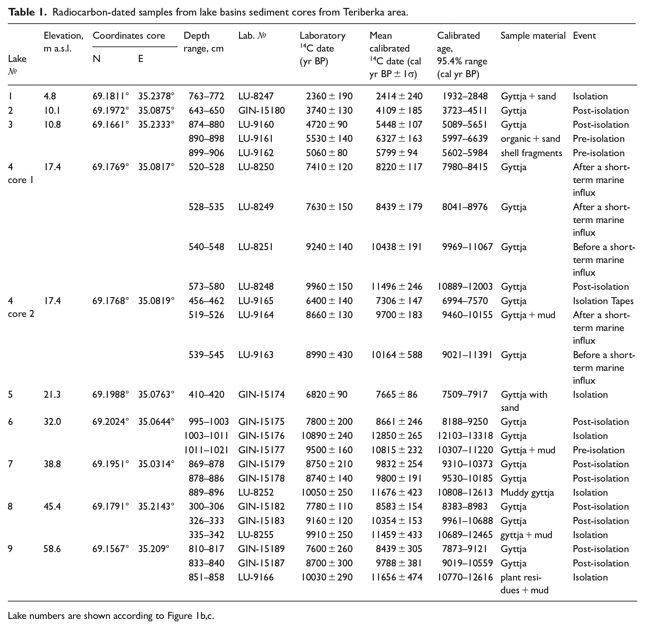
Bulk samples (Table 1) were dated at the laboratory of the St. Petersburg State University (LU samples) and at the laboratory of the Geological Institute of the Russian Academy of Sciences (GIN samples) using the traditional scintillation method, in line with the standard procedures (detailed in Arslanov et al., 1993; Zaretskaya et al., 2005).

Table 1.

Radiocarbon-dated samples from lake basins sediment cores from Teriberka area.

	Elevation, m a.s.l.	Coordinates core		Depth range, cm	Lab. №	Laboratory¹⁴C date (yr BP)	Mean calibrated¹⁴C date (cal yr BP ± 1σ)	Calibrated age,95.4% range (cal yr BP)	Sample material	Event
Lake №	Elevation, m a.s.l.	N	E	Depth range, cm	Lab. №	Laboratory¹⁴C date (yr BP)	Mean calibrated¹⁴C date (cal yr BP ± 1σ)	Calibrated age,95.4% range (cal yr BP)	Sample material	Event
1	4.8	69.1811°	35.2378°	763–772	LU-8247	2360 ± 190	2414 ± 240	1932–2848	Gyttja + sand	Isolation
2	10.1	69.1972°	35.0875°	643–650	GIN-15180	3740 ± 130	4109 ± 185	3723–4511	Gyttja	Post-isolation
3	10.8	69.1661°	35.2333°	874–880	LU-9160	4720 ± 90	5448 ± 107	5089–5651	Gyttja	Post-isolation
				890–898	LU-9161	5530 ± 140	6327 ± 163	5997–6639	organic + sand	Pre-isolation
				899–906	LU-9162	5060 ± 80	5799 ± 94	5602–5984	shell fragments	Pre-isolation
4 core 1	17.4	69.1769°	35.0817°	520–528	LU-8250	7410 ± 120	8220 ± 117	7980–8415	Gyttja	After a short-term marine influx
				528–535	LU-8249	7630 ± 150	8439 ± 179	8041–8976	Gyttja	After a short-term marine influx
				540–548	LU-8251	9240 ± 140	10438 ± 191	9969–11067	Gyttja	Before a short-term marine influx
				573–580	LU-8248	9960 ± 150	11496 ± 246	10889–12003	Gyttja	Post-isolation
4 core 2	17.4	69.1768°	35.0819°	456–462	LU-9165	6400 ± 140	7306 ± 147	6994–7570	Gyttja	Isolation Tapes
				519–526	LU-9164	8660 ± 130	9700 ± 183	9460–10155	Gyttja + mud	After a short-term marine influx
				539–545	LU-9163	8990 ± 430	10164 ± 588	9021–11391	Gyttja	Before a short-term marine influx
5	21.3	69.1988°	35.0763°	410–420	GIN-15174	6820 ± 90	7665 ± 86	7509–7917	Gyttja with sand	Isolation
6	32.0	69.2024°	35.0644°	995–1003	GIN-15175	7800 ± 200	8661 ± 246	8188–9250	Gyttja	Post-isolation
				1003–1011	GIN-15176	10890 ± 240	12850 ± 265	12103–13318	Gyttja	Isolation
				1011–1021	GIN-15177	9500 ± 160	10815 ± 232	10307–11220	Gyttja + mud	Pre-isolation
7	38.8	69.1951°	35.0314°	869–878	GIN-15179	8750 ± 210	9832 ± 254	9310–10373	Gyttja	Post-isolation
				878–886	GIN-15178	8740 ± 140	9800 ± 191	9530–10185	Gyttja	Post-isolation
				889–896	LU-8252	10050 ± 250	11676 ± 423	10808–12613	Muddy gyttja	Isolation
8	45.4	69.1791°	35.2143°	300–306	GIN-15182	7780 ± 110	8583 ± 154	8383–8983	Gyttja	Post-isolation
				326–333	GIN-15183	9160 ± 120	10354 ± 153	9961–10688	Gyttja	Post-isolation
				335–342	LU-8255	9910 ± 250	11459 ± 433	10689–12465	gyttja + mud	Isolation
9	58.6	69.1567°	35.209°	810–817	GIN-15189	7600 ± 260	8439 ± 305	7873–9121	Gyttja	Post-isolation
				833–840	GIN-15187	8700 ± 300	9788 ± 381	9019–10559	Gyttja	Post-isolation
				851–858	LU-9166	10030 ± 290	11656 ± 474	10770–12616	plant residues + mud	Isolation

Lake numbers are shown according to Figure 1b,c.

Purification and concentration of carbonaceous sample included removal of visible organic macro-remnants (1), dissolution of carbonates by treatment with 2% HCl and decanting with distilled water to a neutral medium and complete removal of Ca and Mg (2), extraction of humic acids by treatment with 2% NaOH at 90°C–95°C, separation of the alkaline solution in centrifuge, heating it on bain-marie and admixture with HCl (3); the extracted humic acids were purified with distilled water and dried in a desiccator (4). Coal was obtained from the humic acids sample by pyrolysis; this coal was treated with metallic lithium at 700°C to obtain lithium carbide. Acetylene, obtained from lithium carbide by its dissociation with water, was purified from impurities and water vapour by passing through FeCl₃ + CuCl + H₂SO₄ aqueous solution and KOH and accumulated in catcher contained liquid nitrogen. Benzene was synthesized from treated acetylene on a vanadium-aluminosilicate catalyst preactivated by igniting in a vacuum at 400°C; benzene was purified by holding over concentrated sulphuric acid and was distilled in vacuum. A mixture of scintillators was added to the purified benzene. Measurements were carried out on a liquid scintillation spectrometer ‘Quantulus 1220’ (USA, 2011, serial No DG08118229). Based on the measured activity of the sample and radiation background and modern standard, the radiocarbon age was calculated. Oxalic acid standard was adopted as a modern standard on the recommendation of the US National Bureau of Standards in 1959; a fivefold benzene standard was used.

Radiocarbon dates were calibrated to calendar years using the OxCal 4.4 calibration programme (Bronk Ramsey, 2020) and the IntCal20 calibration plot (Reimer et al., 2020).

Isolation basin stratigraphy model

Isolation basin stratigraphy is based on identification of three major facies units and dating of the isolation contact in the sedimentary successions. Facies units are identified based on the lithological character of the sediments and the contained diatom flora. Following Corner et al. (1999, 2001), three major facies units reflecting major depositional environments are identified: unit I–marine (composed of minerogenic material or minerogenic material with a minor organic content and marine diatoms), II–transitional (during composed by mixed organic-minerogenic or organic sediments, typically laminated) and III–freshwater lacustrine (composed of gyttja and lacustrine diatoms). Most of the basins demonstrate sedimentary succession that includes all three facies units, comprising a regressive I–II–III succession related to the isolation of the lake basins. In lake basin 3 (Figure 1b), mixed sediments (unit I_M) were identified inside marine unit I, indicating disturbance, possibly by tsunami influx (Bondevik et al., 1997; Rasmussen et al., 2018).

A complex sediment succession (I–III–I–II–III) was found in lake 4 basin (Figure 1c). Lacustrine sedimentation (unit III) is interrupted by sedimentation in a brackish-water environment (unit I) due to the re-influx of seawater into the lake basin. In the lower part of these sediments, a mixture of gyttja and sand, rip-up clasts, plant fragments was identified; these deposits appear to have been formed as a result of a tsunami influx. Mentioned succession is interpreted below in a broader context.

Results

Isolation basin stratigraphy: Lithology, age and diatoms

We investigated nine closely spaced lakes located in Teriberka settlement area of 8×4 km between 4.8 and 58.6 m above sea level (a.s.l.) (Figure 1b). Sediment columns were found only in these lake basins, whereas many other lakes explored contained no bottom sediments. Sediment succession from lake 4 (core 1, Figure 1c) was studied earlier (Nikolaeva et al., 2019; Tolstobrov et al., 2018) and re-investigated in the course of these works. Data obtained from all other lake basins are presented for the first time.

Lake 1 (Pervoe Titovskoe, elevation 4.8 ± 1.0 m a.s.l., N 69°10′51.8″ E 035°14′16.2″)

This is a large (1700 m×560 m, 0.64 km²), more than 15 m deep lake with oblong shape, fed and drained by small stream (Figure 1). The lake occupies an irregular depression in bedrock. Boulders and cobbles exposed in the streambed, combined with low relief, suggest a threshold close to present lake level. Coring was carried out at 7.5 m depth at the northern part of the lake. The following stratigraphic units were identified (here and below, the depth is shown from the water level in the lake) (Figure 2):

Figure 2.

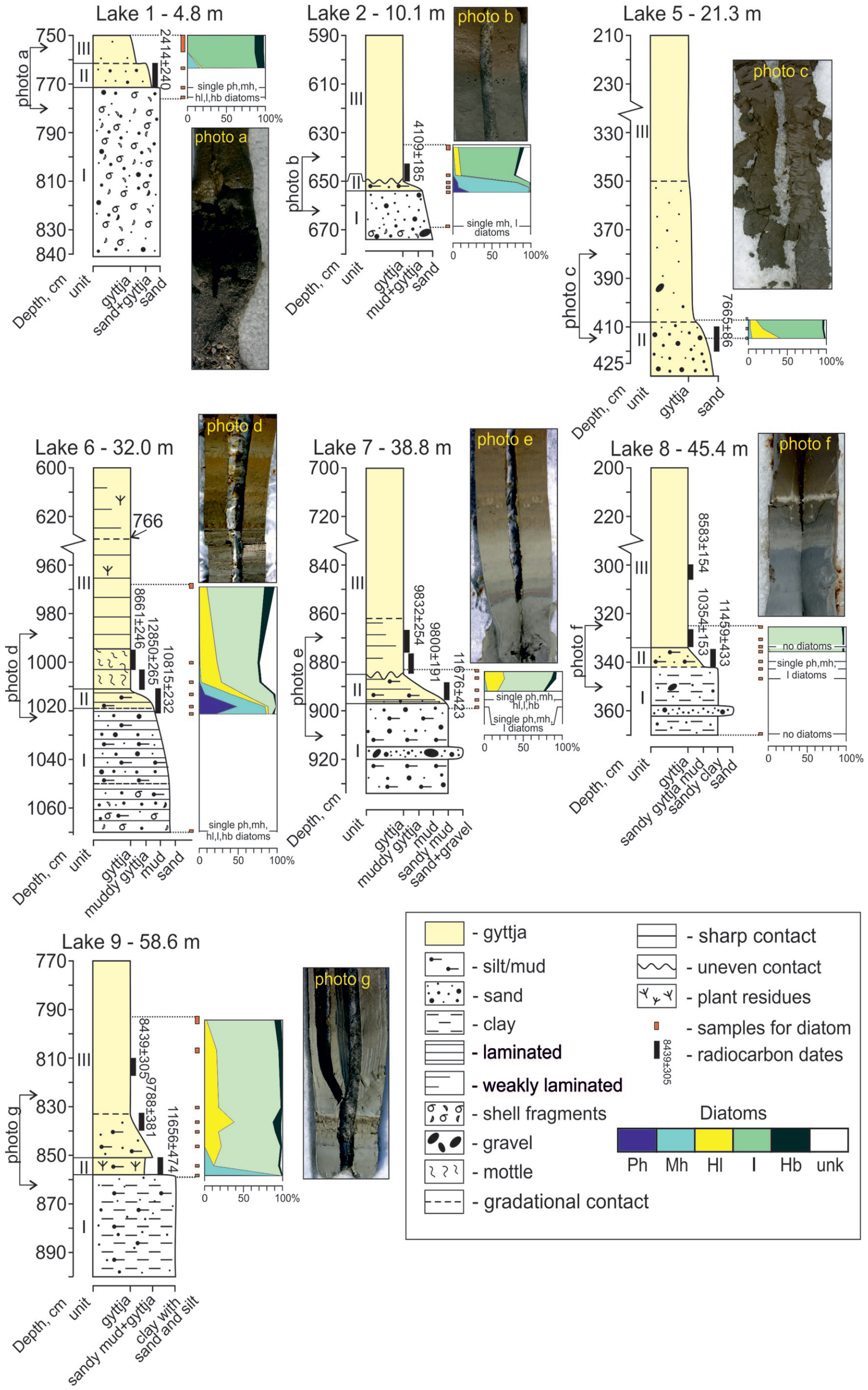
Log of the investigated lakes (numbered according to Figure 1) showing data on lithology, facies, diatoms, radiocarbon dates.

Marine unit I (840–772 cm): shell-rich sand.

Transitional unit II (772–763 cm): massive, dark brown to black sandy gyttja.

Lacustrine unit III (763–750 cm): brown gyttja, structureless, with a small addition of sand.

Lake 1 shows a regressive I–II–III facies succession comprising marine, transitional and freshwater sediments. Single marine and freshwater diatoms were identified in unit I and the lowermost part of unit II. Shell detritus and marine diatom species indicate the marine genesis of unit I, but the presence of freshwater species indicates the influx of fresh water into the basin from streams. The concentration of valves of diatoms increases up the section. The upper part of unit II is dominated by oligohalobous indifferent (71%), together with 16% mesohalobous species, mainly represented by Paralia sulcata (Ehrb.) Kütz. In unit III, mesohalobous species disappear and oligohalobous indifferent and halophobous increase to 98%, indicating a freshwater environment.

Based on lithological and diatom data, the isolation contact is placed at the base of unit III where the diatom flora indicates a change from brackishwater to freshwater conditions. Marine diatoms in underlying unit II suggest tidal influence at that time. A radiocarbon date of 2414 ± 240 cal yr BP (Table 1) from unit II sediments corresponds to a time immediately before isolation.

Lake 2 (Sekretarskoe, elevation 10.1 ± 1.0 m a.s.l., N 69°11′49.5″ E 035°05′15.1″)

This large (1800 m×450 m, 0.70 km²), more than 15 m deep lake is fed by small streams and drained by seepage through a beach barrier to the north (Figure 1). In the lake, the threshold is not obvious; the water level in the lake and the threshold locate at the same elevation under the beach barrier, which is composed of large pebbles and boulders. Lake water easily escapes through this beach barrier threshold; in the northwestern part of lake basin, a small stream was found that opens to daylight beyond the beach barrier at about 9 m a.s.l., according to the topographic map and the ArcticDEM model. Thus, the threshold of lake is at least 9 m a.s.l., which is within the limits of error of ±1 m.

A sediment core was taken in the northern part of the lake from a depth of 5.9 m. The following stratigraphic units are identified (Figure 2):

Marine unit I (674–654 cm): grey sand, massive, with scarce pebbles. Plant macrofossils and shell fragments occur at depth 674–670 cm.

Transitional unit II (654–650 cm): grey muddy gyttja mottled in its upper part.

Lacustrine unit III (650–590 cm): structureless brown gyttja passing upward into watery gyttja.

The I–II–III succession indicates a conformable transition from a marine to a lacustrine environment. Mesohalobous Paralia sulcata (Ehrb.) Kütz. is dominant (67–90%) in the upper part of unit I and in unit II. Other mesohalobous species, such as Rhabdonema minutum Kütz., Navicula digitoradiata (Greg.) Ralfs, Mastogloia elliptica (Ag.) Cl., M. smithii Thw. ex W. Sm., Diploneis smithii (Bréb.) Cl., are also present here. Polyhalobous Plagiogramma staurophorum (Greg.) Heib., Pinnularia quadratarea (A.Schmidt) Cl., Opephora marina (Greg.) Petit, and Lyrella spectabilis (Greg.) D.G. Mann comprise 5–6%. Oligohalobous species increase to 17% in the upper part of unit II. The diatom flora in unit II indicates brackish water conditions. Unit III shows significant changes in the diatom flora. Polyhalobous and mesohalobous species decrease markedly to 0.5–3% in unit III. Oligohalobous indifferent prevail with dominant Stauroforma exiguiformis (Lange-Bert.) Flower, Jones et Round (46% of the total number of valves), as well as Staurosira pseudoconstruens (Marciniak) Lange-Bert., Staurosira construens Ehrb.

The isolation contact is placed between of unit II and unit III where a change in lithology, from sand to gyttja, and a similar change in diatom flora, from predominantly polyhalobous and mesohalobous species to predominantly indifferent species were determined. A date of 4109 ± 185 cal yr BP (Figure 2, Table 1) from the base of the unit III corresponds to the time of post-isolation of the lake from the sea.

Lake 3 (Vtoroe Titovskoe, elevation 10.8 ± 1.2 m a.s.l., N 69°09′57.5″ E 035°13′59.6″)

The lake is oval, 830 m×250 m in size and 0.21 km² in area (Figure 3a). The depth at the coring site is 8.5 m. Small streams drain into and out of the lake in the south-west and north-west, respectively. Boulders and cobbles exposed in the stream bed suggest a threshold located close to the current lake level.

Figure 3.

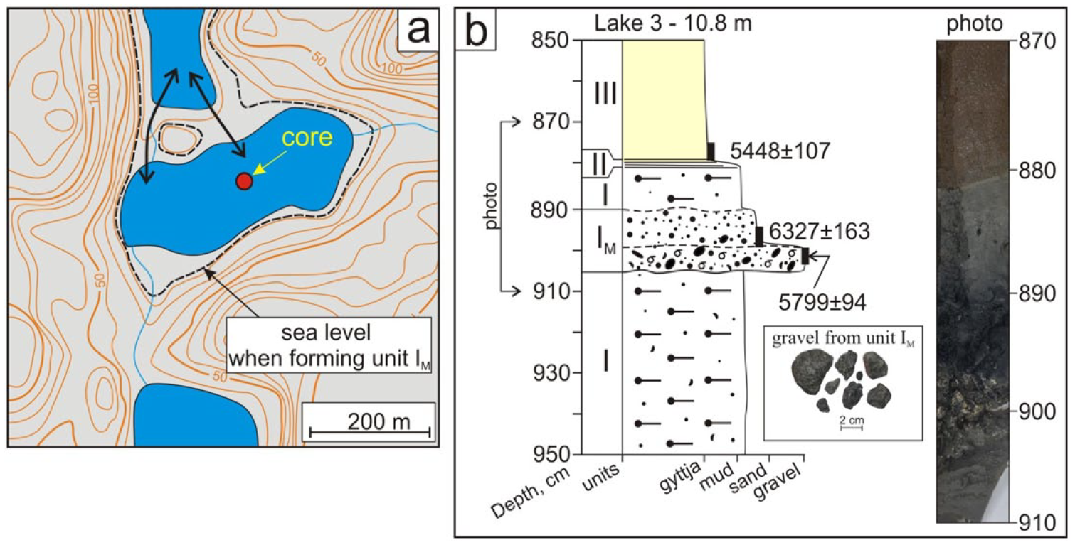
(a) Location map of Lake 3. Core sampling sites is shown as red dot. Sea level is shown with a dotted line during the formation of unit 4. The direction of propagation of the high energy water flow (tsunami) is shown by arrows. (b) Log showing lithology, radiocarbon dates and photo of bottom sediments of Lake 3. See the legend in Figure 2.

The following stratigraphic units are identified (Figure 3b):

Marine unit I (950–880 cm): brownish-grey sandy mud with shell fragments at 950–906 cm, grey sandy mud at the 890–880 cm depth, and mixed unit I_M (906–890 cm) sandy mud including a layer of shells and gravel at 906–899 cm and organic-rich mud at 899–890 cm.

Transitional unit II (880–881 cm): about 1 cm-thick brownish-grey, thinly laminated gyttja mud.

Lacustrine unit III (881–850 cm): structureless brown gyttja passing upward into watery gyttja.

The I–II–III succession indicates a transition from a marine to lacustrine environment. The thin transitional unit II suggests a rapid isolation from the sea. The isolation contact is placed at unit II. The presence of mixed facies (unit I_M) within marine unit I, together with a sharp boundary at the base of unit I_M suggests a break in the succession. The heterogeneous nature of unit I_M, with its content of shells, gravel and organic material indicates a major, high-energy disturbance of sedimentation at some time. Radiocarbon dates of 5799 ± 94 cal yr BP and 6327 ± 163 cal yr BP from unit I_M, at levels 906 to 899 cm and 899–890 cm, respectively, show an inverted age relationship, which further supports the contention that unit I_M contains disturbed sediments. Assuming that the dated material predates the disturbance, these dates suggest that unit I_M was deposited after a maximum of about 6300 yr BP and after or around 5800 yr BP, respectively. Together with a radiocarbon date of 5448 ± 107 cal yr BP (Table 1) from the base of overlying unit III, they suggest that lake 3 was isolated from the sea between about 5800 and 5450 yr BP. Lake 3 occupies a sheltered position so disturbance by storm waves seem unlikely. We suggest that the disturbed sediments in unit I_M were caused by an earthquake or tsunami, when sea level lay slightly higher to the threshold level of 12 m a.s.l. (Figure 3a). Possible evidence for inundation by a tsunami is shown in Figure 3a, which shows traces of a higher shoreline around the lake and the presence of a possible drainage channel breaching the ridge enclosing the lake to the north. We estimate the age of the suggested tsunami event to about 6000 yr BP.

Lake 4 (elevation 17.4 ± 1.0 m a.s.l.)

This small (c. 300 m×140 m, 0.03 km²), 2.5 m deep lake occupies a kettle-hole surrounded by bedrock hills. The lake is fed and drained by small streams about 30 cm deep. Only bedrock is observed in the stream beds and at the threshold, which is located close to the present water level in the lake. The bottom sediments were cored at two sites (Figure 1c). Cores 1 and 2 (N 69°10′37.1″ E 035°04′53.6″ and N 69°10′36.5″ E 035°04′55.0″, respectively) spaced 30 m apart were taken in the central part of the lake.

Core 1

The following stratigraphic units are identified in core 1 (Figure 4):

Figure 4.

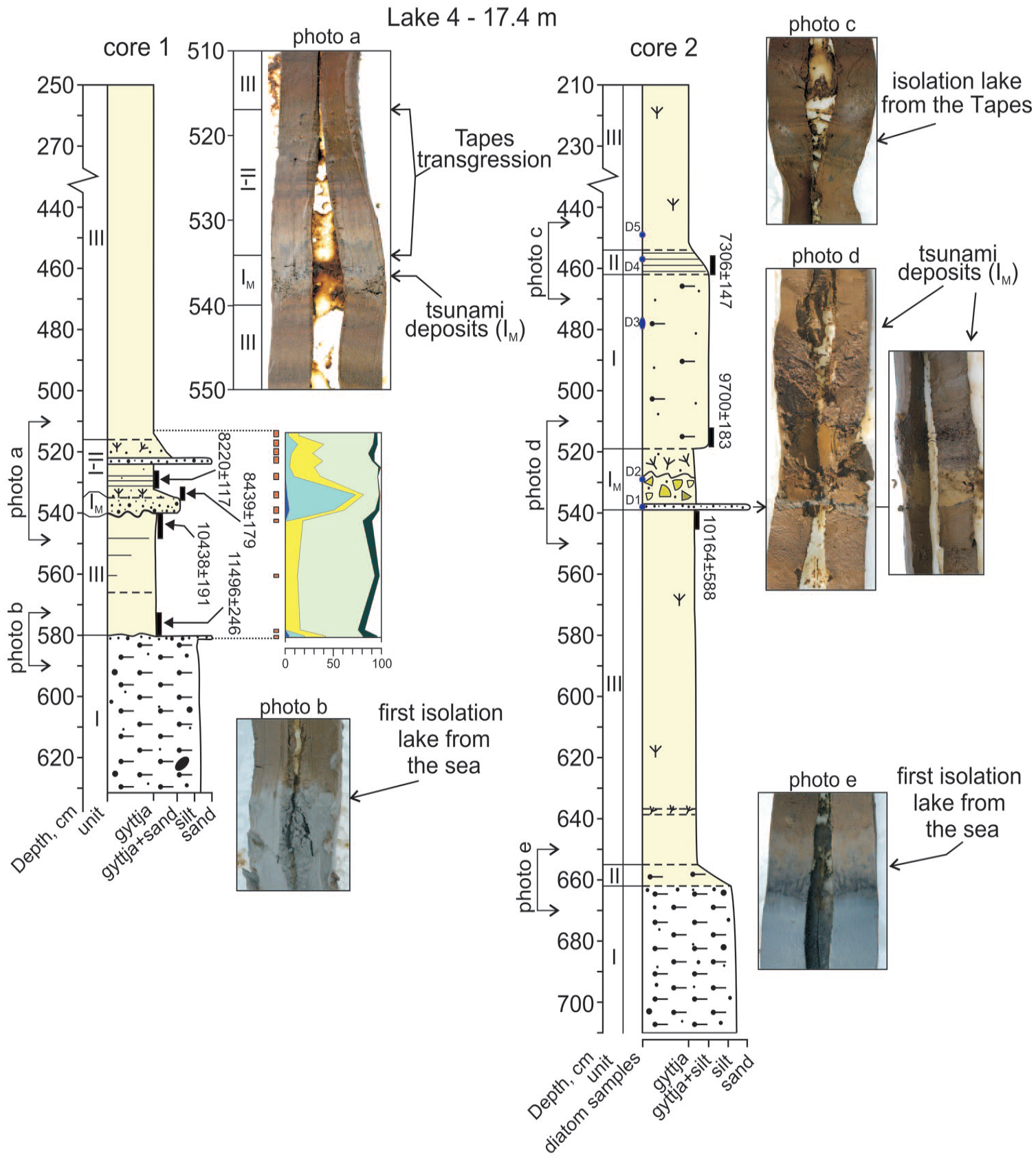
Log of the Lake 4 showing data on lithology, facies, diatoms, radiocarbon dates and photo. See the legend in Figure 2.

Marine unit I (634–580 cm): structureless, grey sandy mud with scarce pebbles; the upper sharp contact is distinct and is marked by a 0.5 cm-thick sandy layer.

Lacustrine unit III (580–540 cm): brown gyttja containing a small quantity of sand; weakly laminated in its upper part (566–540 cm).

Marine unit I – transitional unit II (540–516 cm): , subunit I_M consisting of a gyttja with sand is presented at a 540–535 cm depth; in the lower part, there is almost pure sand; sand content decreases upwards but the content of organic material increases; at a 535–516 cm depth, brown laminated sandy gyttja passing upwards into structureless sandy gyttja with plants macrofossils and sporadic pebbles at a 522–516 cm interval; at a 524–522 cm depth, grey sand lamina up to 2 -cm-thick occurs.

Lacustrine unit III (516–250 cm): brown structureless gyttja with plant remains.

Core 2

The following stratigraphic units are identified in core 2 (Figure 4):

Marine unit I (710–662 cm): structureless, grey sandy mud with scarce pebbles; the upper sharp contact is distinct and is marked by a 0.5 cm-thick sand bed.

Transitional unit II (662–655 cm): muddy gyttja; the colour changes gradually from grey to light brown; black hydrotroilite mottles are also visible.

Lacustrine unit III (655–539 cm): brown gyttja with a small content of sand.

Marine unit I (539–462 cm): subunit I_M presented by grey sand layer (at a 539–538 cm depth), overlain by brown sandy gyttja (sand is up to 5%) with yellowish-brown gyttja fragments (rip-up clasts at a 538–528 cm depth), peat fragments and abundant plant remains (at a 528–519 cm depth) and greyish brown–yellowish brown sandy and silty gyttja with black mottles (at a 519–462 cm depth).

Transitional unit II (462–454 cm): weak laminated brown–yellowish brown sandy and silty gyttja.

Lacustrine unit III (454–210 cm): structureless brown gyttja with plant remains.

Diatoms in core 1 sediments (Figure 4) indicate that the uppermost part of unit I contains marine and brackish water diatoms. Diatoms in overlying lacustrine unit III are exclusively oligoholobous indifferent species (up to 80%). Fragilaria sensu lato is the most common species in this unit. Diatoms in subunit I_M, which erosively overlies unit III, contain marine and brackish diatoms. These increase sharply in this unit, mainly due to an increase in Paralia sulcata (Ehrb.) Kütz. (up to 50–70% of the total number of species). Other mesohalobous species also occur, such as Navicula peregrina (Ehrb.) Kütz., Mastogloia elliptica (Ag.) Cl., as well as polyhalobous Diploneis subcincta (A. Schmidt) Cl., Plagiogramma staurophorum (Greg.) Heib. Brackish-water diatoms are also found in overlying sediments of unit I. Upwards, in unit I and in the lowermost part of unit III, the proportion of mesohalobous and halophilous diatoms gradually decreases, while the number of indifferent and halophobous increases.

Diatoms in core 2 (Figure 4) indicate that sand of subunit I_M (D1, 539–538 cm) is dominated by a variety of freshwater species: Lindavia antiqua (W.Smith) Nakov, Guillory, Julius, E.C.Theriot et alverson, L. radiosa (Grun.) De Toni et Forti, Pantocsekiella schumannii (Grun.) Kiss et Ács, Staurosira construens, Staurosira sp., Rhopalodia gibba (Ehrb.) O. Müll., Eunotia sp., Pinnularia sp. and others. A few marine diatoms are represented by Paralia sulcata, Plagiogramma staurophorum, Diploneis sp. Upward, in the rip-up clasts gyttja of unit I_M (D2 536–535 cm), the diatoms are similar to those from D1 (539 to 538 cm), but the abundance of mesohalobous Paralia sulcata increases. Marine unit I (D3, 482–480 cm) is dominated by marine and brackishwater species, such as Paralia sulcata, Trachyneis aspera (Ehrb.) Cl., Mastogloia sp., Nitzschia sp. and others. A few freshwater species are also found here. In the unit II (D4, 462–461 cm), the abundance of freshwater species increases noticeably, and marine diatoms are also present. Unit III sediments (D5, 450–451 cm) contain only freshwater diatoms.

The stratigraphy of lake 4 comprises an unusual I–II–III–I_M–I–II–III succession in core 2, and succession I–III–I_M–(I–II)–III in core 1. The abrupt change in lithology and diatom flora between units I and III in core 1, together with the presence of a sand layer at the boundary between these units, suggests that the unit I–III boundary is unconformable and that any previously deposited transitional unit II sediments have been removed by slumping or erosion. The diatom flora in units I and III in core 1 nevertheless suggest initial isolation of the basin around the time of deposition of the I to III transition. Radiocarbon dates of 11,496 ± 246 cal yr BP from the base of unit III in core 1 (Figure 4, Table 1) give nominal maximum ages for this initial isolation event.

Units I_M show a sharp increase in marine and brackish diatoms, suggesting a new influx of marine water into the basin. Radiocarbon dates of 10,438 ± 191 cal yr BP (core 1) and 10,164 ± 588 cal yr BP (core 2), from immediately below the unit I_M boundary correspond the maximum age for renewed influx of marine water into the basin. A date of 9700 ± 183 cal yr BP (core 2) from the basal part of unit I in core 2 (Figure 4, Table 1) corresponds to the youngest age for this marine event. Since the boundary between units I_M and I in core 2 is indistinct and uneven, it is possible that some quantity of old organic matter composing unit I_M could have been included in the dated sample. Hence, the date of 9700 ± 183 cal yr BP (core 2) for the end of mentioned marine event could be too old and the date of 8220 ± 117 cal yr BP (core 1) is considered more reliable. We conclude, therefore, that this seawater re-influx occurred sometime between ca. 10,200 and ca. 8200 yr BP. The date of 7306 ± 147 cal yr BP (core 2) from the brackish-water unit II shows that final isolation of the basin probably occurred shortly after ca. 7300 cal. yr BP.

The complex stratigraphy of lake 4 can be explained as resulting from rising sea level following initial isolation of the basin. Irregularities in the succession (Figure 4) could be explained by a possible tsunami influx (detailed in Nikolaeva et al., 2019; Tolstobrov et al., 2018) at the initial phase of the re-connection of the lake with the sea. Based on radiocarbon dates the postulated tsunami sediments (unit I_M) were formed ca. 10,200–8200 cal yr BP. Unit II brackish-water sediments accumulated in the mid-Holocene marine basin until ca. 7300 cal. yr BP.

Lake 5 (elevation 21.3 ± 1.3 m a.s.l., N 69°11′55.6″ E 035°04′34.8″)

This is a small (260 m×170 m, 0.04 km²), oval lake, with a depth of 2.1 m (Figure 1). The lake is fed by atmospheric precipitation and drains via a small stream which cuts through a beach ridge (Tapes beach) located at about 20–22 m a.s.l. to the east. Coring was carried out near the centre of the lake at 2.1 m depth.

The following stratigraphic units are identified (Figure 2):

Transitional unit II (425–408 cm): structureless brown gyttja with sand (50%).

Lacustrine unit III (408–210 cm): sandy gyttja with scarce pebbles (408–350 cm), overlain by brown to dark brown gyttja (350–210 cm).

The core contains an incomplete regressive II–III succession lacking an underlying marine unit I. In unit II, freshwater and brackish-water diatoms include indifferent Stauroforma exiguiformis (Lange-Bert.) Flower, Jones et Round, Staurosira venter (Ehrb.) Kobayasi, etc., as well as halophilous Pseudostaurosira subsalina (Hust.) Morales, Staurosirella pinnata (Ehrb.) Williams et Round, etc. Polyhalobous Plagiogramma staurophorum, Diploneis subcincta and mesohalobous Diploneis interrupta (Kütz.) Cl., D. didyma (Ehrb.) Cl., and Navicula peregrina etc. were also identified in scarce amounts, eventually disappearing in the upper part of unit II, where diatoms are halophobous and indifferent, that is, typical freshwater species.

Diatoms in Lake 5 show that transitional unit II sediments were accumulated under conditions when the sea level lay slightly below the lake threshold. A radiocarbon date from unit II gave an age of 7665 ± 86 cal yr BP (Table 1) which corresponds to a sea level slightly below the threshold.

Lake 6 (elevation 32.0 ± 1.0 m a.s.l., N 69°12′08.6″ E 035°03′52.0″)

This small (450 m×160 m, 0.05 km²), 6 m deep lake occupies an elongated depression between bedrock hills. Drainage into and out of the lake is by small streams. Bedrock exposed in the stream bed suggests a threshold close to present lake level. A core was taken from the central part of the lake, at 6 m depth. The following stratigraphic units are identified (Figure 2):

Marine unit I (1073–1019 cm): dark grey muddy sand and sandy mud, laminated, with sporadic pebbles and layers rich in macro algae remnants; shell fragments occur at 1073–1050 cm depth.

Transitional unit II (1019–1011 cm): laminated unit comprising muddy gyttja, alternating with gyttja and sandy mud. The contact with overlying sediments is abrupt.

Lacustrine unit III (1011–600 cm): brown gyttja with mottle (1011–1003 cm), overlain by light brown to brown gyttja with plant macrofossils, laminated and in the upper part (766-600 cm) weakly laminated.

Lake 6 displays a regressive sequence of sediments and diatoms. Polyhalobous Plagiogramma staurophorum (Greg.) Heib. and mesohalobous Rhabdonema minutum Kütz. diatoms dominate in unit I. Other (scarce) diatoms in this unit are represented by mesohalobous and polyhalobous species, such as Diploneis (D. subcincta (A.Schmidt) Cl., D. chersonensis (Grun.) Cl., D. interrupta (Kütz.) Cl., D. smithii (Bréb.) Cl.), Amphora proteus Greg., Grammatophora angulosa Ehrenb., Navicula digitoradiata (Greg.) Ralfs, Pinnularia quadratarea (A. Schmidt) Cl., and Trachyneis aspera (Ehrb.) Cl. The amount of polyhalobous species decreases sharply in the upper part of unit II. Polyhalobous and mesohalobous almost completely disappear in the unit III gyttja. Unit III is dominated by oligohalobous; while halophilous species Staurosirella pinnata (Ehrb.) Williams et Round, and Cyclotella schumannii (Grun.) Håkans. are gradually replaced by indifferent species Stauroforma exiguiformis (Lange-Bert.) Flower, Jones et Round, Staurosira construens Ehrb., Pinnularia septentrionalis Kramm., Pinnularia subgibba Kramm., Pinnularia viridiformis Kramm. and halophobous Tabellaria flocculosa (Roth) Kütz., Brachysira sp. towards the top of the section.

The isolation contact is placed at the top of unit II laminated sediment, since the diatom flora indicates an abrupt change from marine/brackish to freshwater conditions. However, deformation structures at the base of overlying unit III, together with the abrupt transition suggest that the succession has been disturbed. This is also indicated by the inverted radiocarbon dates of 10,815 ± 232 cal yr BP and 12,850 ± 265 cal yr BP obtained from unit II and the base of unit III, respectively (Table 1). The banding in Unit III presumably reflects periodic changes in lake hydrology following isolation, perhaps caused by storms or disturbance of density stratification by snow avalanching or some other process. A date of 8661 ± 246 cal yr BP gives a minimum age for basin isolation. We place isolation of lake 6 from sea some time during the interval 10,815–12,850 cal yr BP.

Lake 7 (elevation 38.8 ± 1.0 m a.s.l., N 69°11′42.5″ E 035°01′52.9″)

This is a small (380 m×140 m, 0.06 km²) lake with a depth of 7 m. The lake is surrounded on all sides by bedrock hills, except to the east, where a sloping area, drained by a small stream, extends across the outlet. Boulders and cobbles exposed in the stream bed suggest a threshold close to the present lake level. Coring was carried out in the eastern part of the lake at 7 m depth.

The following stratigraphic units are identified (Figure 2):

Marine unit I (934–897 cm): grey sandy mud, structureless; sand with gravel occurs at 920–915 cm depth. The contact with overlying unit II sediments is sharp and uneven.

Transitional unit II (897–885 cm): grey muddy gyttja, weakly laminated, with black mottles. A reddish-brown sandy gyttja layer forms a marked contact with underlying sediments at 896 cm depth. The contact with overlying unit III sediments is sharp and uneven.

Lacustrine unit III (885–700 cm): brown gyttja, with weak lamination and black mottles at the base (885–861 cm depth). This is overlain by laminated gyttja (861–850), which passes upward into homogeneous gyttja (850–700 cm). Lenses enriched with silt are presented at depth 882–880 cm.

The I–II–III succession indicates a conformable transition from a marine to a lacustrine environment. Fragments and single valves of polyhalobous (Diploneis subcincta (A.Schmidt) Cl., Pinnularia quadratarea (A.Schmidt) Cl., Trachyneis aspera (Ehrb.) Cl.), mesohalobous (Rhabdonema minutum Kütz., etc), as well as indifferent (Pinnularia borealis Ehrb., Amphora ovalis (Kütz.) Kütz., and Stauroforma exiguiformis (Lange-Bert.) Flower, Jones et Round) were found in the unit I and in the lower part of unit II. Unit II contains both freshwater and marine diatoms. The amount of diatoms valves increases sharply in the uppermost samples from unit II and in unit III where oligohalobous indifferent (about 60%), including Fragilaria sensu lato, dominate. Diatoms show that the final isolation of lake 7 corresponds to the base of unit II, which was radiocarbon dated to11,676 ± 423 cal yr BP (Table 1), representing a sea level slightly below the threshold level of c. 39.0 m a.s.l. Two dates from unit III postdate isolation.

Lake 8 (elevation 45.4 ± 1.6 m a.s.l., N 69°10′44.7″ E 035°12′51.6″)

This is a small (400 m × 150 m, 0.04 km²) lake with a depth of 2 m. The lake is fed by atmospheric precipitation. Drainage from the lake occurs through a small stream to the west. Bedrock exposed in the stream bed suggests a threshold close to present lake level.

The following stratigraphic units are identified (Figure 2):

Marine unit I (370–342 cm): structureless grey sandy clay with gravel; a layer of sand occurs in the middle part at a depth of 362–358 cm.

Transitional unit II (342–334 cm): sandy gyttja mud, weakly laminated, with black mottles; upwards, the colour gradually changes from light grey to light brown; upper boundary is marked by a thin layer of albescent gyttja.

Lacustrine unit III (334–200 cm): structureless light brown to brown gyttja.

The I–II–III succession indicates a conformable transition from marine to lacustrine environment. No diatoms were found in the lower part of unit I. Single marine diatoms appear in the upper part of unit I. Both freshwater and marine diatoms were found in unit II; freshwater species, such as predominant indifferent Stauroforma exiguiformis (Lange-Bert.) Flower, Jones et Round, occur at the top of unit II. The concentration of diatom valves increases significantly in samples from unit III, where indifferent Stauroforma exiguiformis prevails together with diatoms of genera Frustulia, Eunotia, Pinnularia, and Stauroneis. The isolation contact is placed in the lower part of unit II. A radiocarbon date of 11,459 ± 433 cal yr BP (Table 1) from unit II corresponds approximately to sea level at the threshold, c. 47 m a.s.l, during isolation.

The absence of diatoms in the lower part of unit III could indicate periglacial conditions or strong meltwater input during deglaciation, corresponding in time to dates of between 11,459 ± 433 cal yr BP and 10,335 ± 154 cal yr BP, obtained from units II and III respectively.

Lake 9 (elevation 58.6 ± 1.0 m a.s.l., N 69°09′24.0″ E 035°12′32.4″)

This is a small (510 m×170 m, 0.09 km²), oval-shaped, deep (more than 15 m) lake. The lake is fed by atmospheric precipitation. Drainage from the lake occurs through a small stream (about 30 cm deep) to the east. On the stream bed, boulders and cobbles are observed and the threshold elevation corresponds to water level in the lake. Coring was carried out at 7.7 m depth at the southern end of the lake.

The following stratigraphic units are identified (Figure 2):

Marine unit I (900–858 cm): non-laminated/weakly laminated, grey, sandy and silty clay; a layer rich in filamentous remnants of marine macro-algae occurs at depth of 862–858 cm.

Transitional unit II (858–851 cm): weakly laminated, grey to brownish grey, sandy mud with plant macrofossils and gyttja fragments.

Lacustrine unit III (851–770 cm): structureless grey mud with organic material (gyttja mud), at the base of the unit (851–833 cm) gradually passing into grey muddy gyttja and brown, weakly laminated and non-laminated gyttja (833–770 cm) with a small amount of sand; a layer of whitish-grey gyttja occurs at 810–802 cm.

The I–II–III facies succession represents a change from brackish water to lacustrine phases. No diatoms were found in the lower part of unit I. Concentration of diatoms is very low at the top of unit I, brackish-water Diploneis smithii (Bréb.) Cl., Amphora sp., fragments of Trachyneis aspera (Ehrb.) Cl., and Diploneis sp. are observed. The overlying unit II shows an increased concentration of diatoms, with dominated indifferent species and subdominant mesohalobous diatoms. They indicate an isolation phase with this unit. Mesohalobous diatoms disappear in unit III, oligohalodous indifferent (60–87%) and halophilous (up to 37%) species are most abundant, decreasing to 3% upwards in the succession, where halophobous species increases from 1–3% to 8% in the upper part of unit III. The isolation contact is placed at the top of unit II, radiocarbon dated to 11,656 ± 474 cal yr BP (Table 1) and corresponding approximately to sea level at the threshold c. 58 m a.s.l. Two dates from unit III postdate isolation by a wide margin (Figure 2, Table 1).

Relative sea-level curve

The RSL curve (Figure 5) has been constructed assuming that the radiocarbon dated transitional unit in the lake sediments corresponds to the isolation contact and elevation of the basin threshold, indicating the location of the ancient coastline at the time of isolation from the sea.

Figure 5.

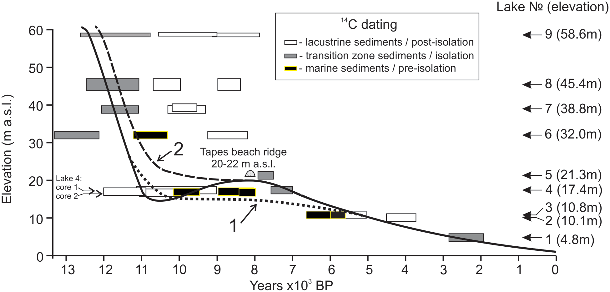
Relative sea-level curve for the Teriberka area based on dated isolation contacts in each of the nine investigated lake basins. The curve refers to calibrated years. Dotted lines show alternative RSL curves, see text for explanation.

The oldest dates, of 11,676 ± 423, 11,459 ± 433 and 11,656 ± 474 cal yr BP from lakes 7, 8 and 9, respectively (Figure 2, Table 1), indicate a sea-level fall from 58 to 39 m a.s.l. and provide evidence of rapid coastline regression related to glacio-isostatic rebound during the Late Glacial and beginning of the Holocene.

Lake 6,which has a threshold elevation at 32.0 m a.s.l., shows an inversion in the age of two closely located sedimentary intervals (Figure 2, Table 1), likely caused by the mixing of sediments through slumping. We infer that isolation of this lake occurred sometime between the obtained two dates, that is, during time interval 10,815–12,850 cal yr BP.

In the sedimentary successions from lakes 1, 2, 3 and 5, located 4.8, 10.1, 10.8 and 21.3 m a.s.l., respectively, isolation or post-isolation contacts were radiocarbon dated to 2414 ± 240 cal yr BP, 4109 ± 185 cal yr BP, 5448 ± 107 cal yr BP and 7665 ± 86 cal yr BP. At those times, sea level was located close to or slightly below threshold level in the mentioned lakes.

Three transitional units were identified in the sedimentary succession from lake 4. The first records initial isolation of the basin from the sea. A date of 11,496 ± 246 cal yr BP from the overlying gyttja unit gives a post-isolation age that is probably close to the actual age of isolation (Figure 4, Table 1). Repeated flooding of this lake basin by sea water was caused by the Tapes marine transgression and some sediment was eroded. The Tapes transgression occurred in the interval approximately 10000–7000 cal yr BP (Fjeldskaar and Bondevik, 2020) in areas where intense glacioisostatic uplift has ceased, but the sea level continued to rise initiated by a meltwater pulse into the North Atlantic (LeGrande et al., 2006) as a result of final demise of the Laurentide Ice Sheet (Carlson et al., 2008; PALSEA (PALeo SEA level working group), 2010). Corresponding sediments and landforms have been found in many coastal areas of Fennoscandia, including the Barents and White Seas coasts (Kolka et al., 2013; Møller et al., 2002; Snyder et al., 2008b). Previously, the Tapes transgression-maximum shorelines (beach ridges) were identified at an elevation of 20–25 m a.s.l. near the Teriberka area (Koshechkin 1979; Snyder et al., 2008b), and they are well traced on satellite images and digital models of the Earth. In the Teriberka area, the Tapes shoreline was found at an elevation of about 20–22 m a.s.l. in one of the studied lake basin, that is, in lake 5 basin.

The final isolation of the lake 4 after the Tapes transgression corresponds to an isolation contact (at the depth 462–454 cm) dated to 7306 ± 147 cal yr BP.

Discussion

In the Kola region, RSL changes were mainly defined by glacio-isostatic rebound during deglaciation and the Holocene. The oldest dates of 11,676 ± 423, 11,459 ± 433 and 11,656 ± 474 cal yr BP for unit II in sedimentary sequences from lakes 7, 8 and 9 provide reliable evidence that Teriberka area was deglaciated earlier than 12,000 cal yr BP. This is consistent with the location of end moraines in the Kola region (Korsakova et al., 2023a) and in the Teriberka area, with marginal glacial landforms that are comparable to the Neva or Keiva II stades (c. 13,900–14,100 cal yr BP). This is also indicated by the dates of 12,955–13,960 cal yr BP for lake sediments in the Dalnie Zelentsy area (Snyder et al., 2008a).

In the Teriberka area, basal sandy and silty clays without diatoms in the sedimentary successions from lakes 8 and 9 indicate that the lower part of marine unit I accumulated during the terminal phase of deglaciation in severe Late Glacial conditions. Their accumulation could be associated with the Younger Dryas cooling (12900-11700 years ago). Sea level at the end of deglaciation was located at c. 59 m a.s.l., as shown by the altitude-age reconstruction based on data from lake 9 bottom sediments. The RSL curve (Figure 5) shows a rapid fall in sea level, at a rate of about 40 mm per year, during the Late Glacial and early Holocene. At about 11,500 cal yr BP, RSL fell below an altitude of 17 m a.s.l., as shown by data from lake 4. It then rose by more than 5 m between c. 10,000 and 7600 cal yr BP during the Tapes transgression, reaching a peak of about 21 m a.s.l., as suggested by the data from lakes 4 and 5. In addition, at an elevation of about 20–22 m a.s.l., well-shaped beach ridges were observed, which formed at the peak of the mid-Holocene Tapes transgression. The post-7300 years part of the RSL curve shows a gradual fall in sea level at a rate of about 2–3 mm per year.

Disturbed sediments were found in lakes 3 and 4 (Figures 3 and 4). We interpret them as having formed as a result of a tsunami. Similar sediments generated by a tsunami have been noted in a number of lakes around the North Atlantic (Bondevik et al., 1997; Romundset et al., 2011). These sediments could be associated with the Storegga tsunami triggered by offshore slumping about 8200 cal. yr BP. Based on new dates (Table 1), the age of disturbed sediments in lakes 3 and 4 is about 6000 cal. yr BP and 10,200–8200 cal. yr BP, respectively. The sediments of unit II_A in lake 4 have a similar lithology to the Storegga tsunami sediments described in western Norway (Bondevik et al., 1997), suggesting a similar genesis and age, although the position and orientation of the Teriberka coast would suggest that such a correlation is unlikely. It can’t be excluded, however, that others paleoseismic (earthquake) events occurred in the study area and caused tsunamis. Records of such paleoseismic events were studied on the Barents Sea coast of the Kola Peninsula (Nikolaeva, 2008, 2009; Nikonov and Shvarev, 2015; Verzilin et al., 2013 etc.) and are shown by faults and ruptures in the bedrock, as well as deformed horizons of loose sediments.

Noteworthy, according to the modelling of the Tapes transgression along the Norwegian coast (Fjeldskaar and Bondevik, 2020), there should be no Tapes transgression in the Kola region, with the except of the easternmost Kola peninsula, because of too high rates of uplift rates there. Therefore, we tried to construct alternative RSL curves for the Teriberka area (Figure 5). If we assume that there should only be tsunami deposits in lake 4, it turns out that RSL was located below 17 m about 11,000 years ago, that is, below the threshold from lake 4 (alternative RSL curve shown by the dotted line 1 in Figure 5). In this case, it is incomprehensible when the coastal landforms clear recorded at elevation of 20–22 m were formed. It is quite reasonable that these coastal landforms should be associated with the Tapes transgression. In addition, the radiocarbon dating data of sediments represented by gyttja with brackish-water diatoms from lakes 5 and 4 do not agree with this alternative RSL curve. If we assume that the sea level did not fall below the lake 4 threshold (RSL curve shown dotted line 2 in Figure 5), the alternative RSL curve is consistent with the location of mentioned coastal landforms, but does not consistent with radiocarbon dating data of freshwater sediments from lake 4 in the time interval of 11,000–10,000 years ago. From all of the above, we propose the RSL curve with a transgressive phase (solid line in Figure 5).

Figure 6 shows the RSL curve reconstructed for Teriberka area together with those previously reconstructed in comparable coastal areas: Dalnie Zelentsy (Snyder et al., 2008a), Nikel – Kirkenes (Corner et al., 1999) and Polyarny (Corner et al., 2001). The four RSL curves for the north-west Kola Peninsula (Figure 6) show a pattern of glacio-isostatic uplift which conforms predictably to the position of each site relative to the margin of the retreating Fennoscandian Ice Sheet. The amplitude of glacio-isostatic uplift increases from east to west, that is, in a direction from the Dalnie Zelentsy area to the Nikel–Kirkenes area. The initial rapid postglacial emergence indicates pronounced glacio-isostatic rebound shortly after deglaciation. There are differences in the timing of the maximum rate of uplift depending on the time of retreat of the eastern Fennoscandian ice sheet. In both the Dalnie Zelentsy and Teriberka areas, the maximum uplift rate occurred during the time interval 12,000–11,500 cal yr BP. In a westward direction, the maximum uplift rate was achieved at the later time: 10,500–10,000 cal yr BP and 10,200–9800 cal yr BP in the Polyarny and Nikel-Kirkenes areas, respectively (Corner et al., 1999, 2001). The maximum rate of glacio-isostatic uplift, which is a function of glacial rebound and the Earth’s rheology, is assumed to occur approximately 1500–2000 years after deglaciation. This assumption is supported by seismic events and faulting which appear to correspond to the time of maximum uplift. Thus, in the Murmansk area, deglaciated approximately 12,500–12,000 cal yr BP (Figure 1b), a seismic event was recorded at approximately 10,000 cal yr BP (Nikolaeva, 2008). Evidence is also provided by postglacial rock-slope failures formed 1600–1700 years after deglaciation, as described in Scotland and NW Ireland (Ballantyne et al., 2014).

Figure 6.

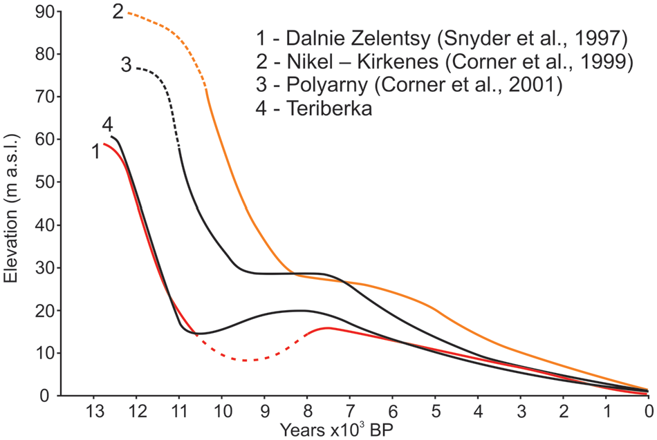
Relative sea-level curve for the Teriberka area compared with curves constructed for others coastal areas, adjusted for differences between radiocarbon years and calibrated years: Nikel-Kirkenes (Corner et al., 1999), Polyarny (Corner et al., 2001) and Dalnie Zelentsy (Snyder et al., 2008a).

In the Early to Mid-Holocene on the Varanger Peninsula coast (Romundset et al., 2011), and in the Dalnie Zelentsy area (Snyder et al., 2008a) and at Teriberka, a low-amplitude (2–5 m) transgression cresting at 7500 cal yr BP was reconstructed. In the Nikel-Kirkenes and Polyarny areas, only a prolonged stillstand is shown at this time. A similar pattern, in which the Tapes transgression is well manifested on outer sea coasts and islands, while being represented only by a coastal stillstand at the head of large gulfs, was noted in western Norway (Svendsen and Mangerud, 1987) and northern Europe (Lambeck et al., 1998). In areas close to the centre of the last ice sheet, only marine regression occurred in the Holocene (Berglund, 2004).

Conclusions

Based on new lithostratigraphical, diatom and radiocarbon data, a RSL curve was constructed for the Teriberka area on the Barents Sea coast. It shows that RSL fell rapidly at a rate of about 40 mm per year during the Late Glacial and early Holocene. About 11,500 cal yr BP, the RSL fell below to 17 m and then rose by more than 5 m during the Tapes transgression (10,000–7600 cal yr BP). At the maximum of the Tapes transgression, the sea coastline located slightly below the elevation 22 m a.s.l. After 7300 cal yr BP, a gradual regression occurred at an average rate of about 2–3 mm per year.

Footnotes

Acknowledgements

This paper was initiated by the first author before he passed away on 23th April 2020. The final editing was carried out by Dmitry Tolstobrov who worked for the last ten years with Vasily Kolka and by Geoffrey D. Corner with whom Vasily Kolka began his researches on RSL changes in the Kola region at the end of the 20th Century, which continued for many years. We dedicate this paper to the memory of Dr. Vasily Kolka.

Funding

The author(s) disclosed receipt of the following financial support for the research, authorship, and/or publication of this article: The research was supported by the Ministry of Science and Higher Education of the Russian Federation project АААА-А19-119100290145-3. The work was partly supported by the Ministry of Education of the Russian Federation (project No. FSZN–2020–0016, VRFY-2023-0010). We are grateful to our colleagues from the Geological Institute of the Kola Science Centre of Russian Academy of Sciences (GI KSC RAS) for their help during the fieldwork in 2013, 2016 and 2018.

ORCID iD

Dmitry Tolstobrov

References

Arslanov

Tertychnaya

Chernov

(1993) Problems and methods of dating Low-Activity samples by liquid scintillation counting. Radiocarbon 35: 393–398.

Ballantyne

Sandeman

Stone

, et al. (2014) Rock-slope failure following Late pleistocene deglaciation on tectonically stable mountainous terrain. Quaternary Science Reviews 86: 144–157.

Barinova

Medvedeva

Anisimova

(2006) Biodiversity of algae-indicators of environments. Pilies Studio, Tel-Aviv; 498. in Russian.

Berglund

(2004) Holocene shore displacement and chronology in ångermanland, eastern Sweden, the Scandinavian glacio-isostatic uplift centre. Boreas 33: 48–60.

Bondevik

Inge Svendsen

Mangerud

(1997) Tsunami sedimentary facies deposited by the Storegga tsunami in shallow marine basins and coastal lakes, western Norway. Sedimentology 44: 1115–1131.

Bronk Ramsey

(2020) OxCal 4.4 [Online resource]. Available at: http://c14.arch.ox.ac.uk. (accessed 14 October 2020).

Carlson

LeGrande

Oppo

, et al. (2008) Rapid early holocene deglaciation of the laurentide ice sheet. Nature Geoscience 1: 620–624.

Corner

Kolka

Yevzerov

, et al. (2001) Postglacial relative sea-level change and stratigraphy of raised coastal basins on Kola Peninsula, northwest Russia. Global and Planetary Change 31(1-4): 155–177.

Corner

Yevzerov

Kolka

, et al. (1999) Isolation basin stratigraphy and holocene relative sea-level change at the Norwegian-Russian border north of Nikel, northwest Russia. Boreas 28(1): 146–166.

10.

de Geer

(1890) Om Skandinaviens niråförändringar under qvartär-perioden. Geologiska Föreningeni Stockholm Förhandlingar 12(2): 61–110.

11.

Donner

Eronen

Jungner

(1977) The dating of the Holocene relative sea-level changes in Finnmark, North Norway. Norsk Geografisk Tidsskrift 31(3): 103–128.

12.

Fjeldskaar

Bondevik

(2020) The Early-Mid Holocene transgression (Tapes) at the Norwegian coast – Comparing observations with numerical modelling. Quaternary Science Reviews 242: 106435.

13.

Gleser

Makarova

Moiseeva

, et al. (1992) The Diatoms of the USSR (Fossil and Recent), vol. II. St. Petersburg: Nauka, pp.1–125. in Russian.

14.

Goretskiy

(1941) On the role of local geographical environment in the Quaternary history (in case study valleys of rivers Tuloma and Kola, Kola Peninsula). Problemy fizicheskoy geografii: 55–73. in Russian.

15.

Guiry

(2022) AlgaeBase. World-Wide Electronic Publication. Galway: National University of Ireland. http://www.algaebase.org

16.

Hafsten

(1960) Pollen-analytical investigations in South Norway. In: Holtedahl

(ed.) Geology of Norway, Norges Geologiske Undersøkelse. Oslo: H. Aschehoug, pp.434–462.

17.

Högbom

(1913) Handbuch der Regionalen Geologie. Heidelberg: Carl Winter’s universitätsbuchhandlung.

18.

Hustedt

(1957) Die Diatomeenflora des Fluß-systems der Weser im Gebiet der Hansestadt Bremen. Abhandlungen der Naturwissenschaftlichen Verein zu Bremen 34(3): 181–440.

19.

Kalabin

(1999) Ekologicheskiy atlas Murmanskoy oblasti (Ecological atlas of the Murmansk Region). INEP RSC RAS, Moscow-Apatity. in Russia.

20.

Kjemperud

(2008) Diatom changes in sediments of basins possessing marine-lacustrine transitions in Frosta, Nord-Trøndelag, Norway. Boreas 10(1): 27–38.

21.

Kolka

Yevzerov

Møller

, et al. (2013) The late Weichselian and holocene relative sea-level change and isolation basin stratigraphy at the Umba settlement, southern coast of Kola Peninsula. Izvestiya Rossiiskoi Akademii Nauk. Seriya Geograficheskaya (1): 73–88. DOI: 10.15356/0373-2444-2013-1-73-88. (in Russian).

22.

Korsakova

Vashkov

Nosova

(2023a) European Russia: glacial landforms during deglaciation. In: Palacios

Hughes

Garcia-Ruiz

, et al. (eds) European Glacial Landscapes. The Last Deglaciation. Amsterdam, Oxford, Cambridge: Elsevier, pp.105–110.

23.

Korsakova

Vashkov

Nosova

(2023b) European Russia: Glacial landforms from the Younger Dryas stadial. In: Palacios

Hughes

Garcia-Ruiz

, et al. (eds) European Glacial Landscapes. The Last Deglaciation. Amsterdam, Oxford, Cambridge: Elsevier, pp.467–472, DOI: 10.1016/B978-0-323-91899-2.00014-0

24.

Koshechkin

(1979) Tectonics of the eastern part of the Baltic Shield during the Holocene. Nauka, Leningrad: 158. in Russian.

25.

Kremenetski

Vaschalova

Goriachkin

, et al. (2008) Holocene pollen stratigraphy and bog development in the western part of the Kola Peninsula, Russia. Boreas 26(2): 91–102.

26.

Lambeck

Smither

Johnston

(1998) Sea-level change, glacial rebound and mantle viscosity fornorthern Europe. Geophysical Journal International 134(1): 102–144.

27.

Lavrova

(1960) The Quaternary geology of the Kola Peninsula. Moscow-Leningrad: Academy of Sciences of USSR Press, pp.1–234. in Russian.

28.

LeGrande

Schmidt

Shindell

, et al. (2006) Consistent simulations of multiple proxy responses to an abrupt climate change event. Proceedings of the National Academy of Sciences USA 103: 837–842.

29.

Marthinussen

(1974) Contributions to the Quaternary geology of north-easternmost Norway and the closely adjoining foreign territories. Norges Grologiske Undersekelse 3(15): 1–157.

30.

Mitrofanov

(Ed.)(1996) Geological Map of the Kola region, Scale 1:500 000. GI KSC RAS, Apatity.

31.

Møller

Yevzerov

Kolka

, et al. (2002) Holocene raised-beach ridges and sea-ice-pushed boulders on the Kola peninsula, northwest russia: indicators of climatic change. The Holocene 12(2): 169–176. DOI: 10.1191/0959683602hl532rp

32.

Niemelä

Ekman

Lukashov

(1993) Quaternary Deposits of Finland and Northwestern Part of Russian Federation and Their Resources. Map 1: 1 000 000. Espoo – Petrozavodsk. Geological Survey of Finland and Russian Academy of Science, Institute of Geology, Petrozavodsk.

33.

Nikolaeva

Tolstobrov

Tolstobrova

(2019) Disturbances in the primary stratigraphy of lake sediments on the Murmansk coast (Russia): Their identification and relationship with catastrophic events. Baltica 32(2): 156–169.

34.

Nikolaeva

(2008) Disastrous earthquakes in the vicinities of the town of Murmansk: Paleoseismological and geological evidence. Journal of Volcanology and Seismology 2(3): 189–198.

35.

Nikolaeva

(2009) Seismites in late Pleistocene and holocene deposits of the northwestern Kola region (northern Baltic shield). Russian Geology and Geophysics 50(7): 644–650.

36.

Nikonov

(1964) The Relief Development and the Anthropogene Palaeogeography in the West Kola Peninsula. Leningrad: Nauka, pp.1–183.

37.

Nikonov

Shvarev

(2015) Seismolineaments and destructive earth-quakes in the Russian part of the Baltic shield: new solutions for the past 13 thousand years. Materialy Mezhdunarodnoi konferentsii Geologo-geofizicheskaia sreda i raznoobraznye proiavleniia seismichnosti. Izd-vo Tekhnicheskogo instituta SVFU Neriungri: 243–251. in Russian.

38.

PALSEA (PALeo SEA level working group) (2010) The sea-level conundrum: Case studies from palaeo-archives. Journal of Quaternary Science 25: 19–25.

39.

Porter

Morin

Howat

, et al. (2018) ArcticDEM. Harvard Dataverse, V1. DOI: 10.7910/DVN/OHHUKH.

40.

Proshkina-Lavrenko

Glezer

Makarova

(1974) Diatoms of the USSR: Fossil and Modern, vol. I. Leningrad: Nauka, p.403.

41.

Ramsay

(1898) Über die geologische Entwicklung der Halbinsel Kola in der Quartärzeit. Miteiner Karte und fiinf Tafeln. Fennia 16(1): 1–151.

42.

Ramsay

(1924) On relations between crustal movements and variations of sea-level during the Late Quaternary time especially in Fennoscandia. Fennia 44(5): 1–39.

43.

Rasmussen

Bondevik

Corner

(2018) Holocene relative sea level history and Storegga tsunami run-up in Lyngen, northern Norway. Journal of Quaternary Science 33(4): 393–408.

44.

Reimer

Austin

WEN

Bard

, et al. (2020) The IntCal20 Northern Hemisphere radiocarbon age calibration curve (0–55 cal kBP). Radiocarbon 62(4): 725–757.

45.

Romundset

Bondevik

Bennike

(2011) Postglacial uplift and relative sea level changes in Finnmark, northern Norway. Quaternary Science Reviews 30(19-20): 2398–2421.

46.

Snyder

Forman

Mode

, et al. (2008a) Postglacial relative sea-level history: Sediment and diatom records of emerged coastal lakes, north-central Kola Peninsula, Russia. Boreas 26(4): 329–346.

47.

Snyder

Korsun

Forman

(2008b) Postglacial emergence and the tapes transgression, north-central Kola Peninsula, Russia. Boreas 25(1): 47–56.

48.

Stroeven

Hättestrand

Kleman

, et al. (2016) Deglaciation of Scandinavia. Quaternary Science Reviews 147: 91–121.

49.

Svendsen

Mangerud

(1987) Late Weichselian and holocene sea-level history for a cross-section of western Norway. Journal of Quaternary Science 2: 113–132.

50.

Tanner

(1930) Studier öfver kvartärsystemet i Fennoskandians nordliga delar IV. Résumé en français. Bulletin de la Commission géologique de Finlande 88: 1–589.

51.

Tanner

(1936) Det senglaciala havets utbredning i Lutto och suomu älvars dalgångar ovanför sammanflödet samt några ord om morfologin i denna trakt. Résumé: L’extension de la mer senglaciaire dans les vallées des rivières Lutto et suomu en laponie en amont de leur confluent. Bulletin de la Commission géologique de Finlande 115: 107–119.

52.

Terziev

Girdyuk

Zykova

, et al. (1990) Hydrometeorology and Hydrochemistry of the Seas of the USSR, Vol. 1: Barents Sea. Part 1. Hydrometeorological Conditions. Leningrad: Gidrometeoizdat Press, p.280.

53.

Tolstobrov

Kolka

(2019) New schemes of isobases of uplift of northeastern Fennoscandia for the last 10,000 years. Vestnik IG Komi UB RAS 11: 3–8.

54.

Tolstobrov

Tolstobrova

Kolka

, et al. (2018) Putative records of the Holocene tsunami in lacustrine bottom sediments near the Teriberka settlement (Kola peninsula, Russia). Limnology and oceanology Series 9: 92–102.

55.

Verzilin

Bobkov

Kulkova

, et al. (2013) The age and formation of the recent dissected relief of the northern Kola Peninsula. Vestnik SPbGU. Ser. 7. Geol. Geogr 2: 79–93.

56.

Vorren

Plassen

(2002) Deglaciation and palaeoclimate of the Andfjord-Vagsfjord area, North Norway. Boreas 31(2): 97–125.

57.

Zaretskaya

Zhilin

Karmanov

, et al. (2005) Radiocarbon dating of wetland archeological sites whithin the Upper Volga and Middle Vychegda. Geochronometria 24: 117–131.