A low-frequency summer temperature reconstruction for the United States Southwest,3000 BC

Abstract

Temperature variability likely played an important role in determining the spread and productive potential of North America’s key prehispanic agricultural staple, maize. The United States Southwest (SWUS) also served as the gateway for maize to reach portions of North America to the north and east. Existing temperature reconstructions for the SWUS are typically low in spatial or temporal resolution, shallow in time depth, or subject to unknown degrees of insensitivity to low-frequency variability, hindering accurate determination of temperature’s role in agricultural productivity and variability in distribution and success of prehispanic farmers. Here, we develop a model-based modern analog technique (MAT) approach applied to 29 SWUS fossil pollen sites to reconstruct July temperatures from 3000 BC to AD 2000. Temperatures were generally warmer than or similar to those of the modern (1961–1990) period until the first century AD. Our reconstruction also notes rapid warming beginning in the AD 1800s; modern conditions are unprecedented in at least the last five millennia in the SWUS. Temperature minima were reached around 1800 BC, 1000 BC, AD 400 (the global minimum in this series), the mid-to-late AD 900s, and the AD 1500s. Summer temperatures were generally depressed relative to northern hemisphere norms by a dominance of El Niño-like conditions during much of the second millenium BC and the first millenium AD, but somewhat elevated relative to those same norms in other periods, including from about AD 1300 to the present, due to the dominance of La Niña-like conditions.

Keywords

ENSO late-Holocene modern analog technique pollen summer temperatures US Southwest

Introduction

The role that temperature variability plays in shaping prehistoric human population sizes and distributions, agricultural practices, and the success of farming societies is likely underappreciated (d’Alpoim Guedes et al., 2016; Fagan, 2000; Mann, 2002; Peregrine, 2020; Vierra and Vint, 2022). For a long time in fact social researchers in many disciplines paid little attention to climate in general and temperature in particular. Prominent social historian Emmanuel Le Roy Ladurie helped legitimize such research in the social sciences by underscoring the connection between climate and economies over the last millenium (while stopping short of adopting a deterministic perspective): “Climate is no longer looked at for its own sake but ‘as it is for us,’ as the ecology of man. . .. Temperature curves may well connect with general history . . . rainfall curves belong . . . to local or regional history” (Le Roy Ladurie, 1971: 22, 89). Indeed, there is evidence that on global spatial and long temporal scales, human population sizes and distributions, and the locations of highest productivity for crops, livestock, and GDP, are closely tuned to mean annual temperatures (Burke et al., 2015; Xu et al., 2020).

For some time, scholars have been aware of the significant temperature variability throughout the Holocene, with the prime example of the Little Ice Age in Europe (LIA; fifteenth to nineteenth centuries AD) (Mann, 2021; Matthes, 1939), which had well documented negative impacts on crops, livestock, and human health, leading to starvation, famine, and disease (Fagan, 2000; Mann, 2002; White, 2017). It has even been claimed that between AD 1000 and 1980, periods of colder temperatures in Europe helped precipitate frequent conflict (Tol and Wagner, 2010). A recent attempt to confirm this finding using updated statistical methods (Carleton et al., 2021), however, finds no evidence for a causal role for temperature, perhaps because the dominant staple crop in Europe – wheat (Triticum sp.) – is less temperature-sensitive than either rice (Oryza sp.) or maize (Zea mays L.).

Oddly – since in the Americas the more-temperature-sensitive maize was the dominant crop fueling the agricultural demographic transition – the role of temperature variability in the late-Holocene prehistory of the Americas is not so widely discussed. Since maize is a tropical cultigen (Benz, 2006), its movement northwards from its locale of domestication in the Balsas Depression of Mexico has been accompanied by selection for adaptation to greatly reduced growing seasons. Swarts et al. (2017) have shown that selection for earlier flowering had already taken place in 1900-year-old maize from the Basketmaker II sediments of Turkey Pen Shelter in Southeast Utah, although the maize grown there then was still only marginally adapted to the locally available growing degree days. Therefore, summer heat (in addition to adequate moisture) was a critical and probably often limiting component of maize success in the US Southwest, especially in the cooler uplands. The possibility of short growing seasons in the first centuries AD has been invoked as a possible explanation for the slow uptake of maize in the upland Southwest and the long Neolithic (agricultural) demographic transition (approximately 1600 years) in this region (Kohler and Reese, 2014). Since the Basketmaker II populations of Southeast Utah – contemporaneous with the Turkey Pen sediments from which the maize analyzed by Swarts was derived – were already heavily reliant on maize (Coltrain and Janetski, 2013), and since maize likely constituted a remarkable 90% of calories just prior to the depopulation of the northern Southwest in the AD 1200s (Matson, 2016), we must understand temperature history to understand the history of farmers in the prehispanic upland Southwest.

Much of the work linking climate to maize production over the last two millennia in North America has relied on tree-ring-based estimates of soil moisture using the Palmer Drought Severity Index (PDSI). In some cases, these estimates have been derived for particular localities using relatively local tree-ring records (Kohler, 2012; Van West, 1994) but more often they have relied on a large network of tree-ring chronologies spanning North America to make PDSI estimates at regularly spaced (though rather distant) grid points (Cook et al., 2007, 2010). For example, Benson et al. (2007) used these estimates to identify warm droughts (negative PDSI anomalies) between AD 990 and 1060, 1135 and 1170, and 1276 and 1297 (associated with the Medieval Warm Period [MWP] of the eleventh to fourteenth centuries AD). They suggested that these episodes had far-reaching effects on a number of populations in the US Southwest and Midwest because they reduced or eliminated yields from farming.

In the 1980s, Stephen Williams introduced the term “Vacant Quarter” to characterize the near abandonment of large portions of midcontinental United States by late-Mississippian populations, putatively associated with the generally colder temperatures of the LIA (Williams, 1983). A later analysis of population size as reconstructed from summed probability distributions of 14C dates for five regions in the Vacant Quarter, and for the site of Cahokia and its environs, seemed to show only a weak relationship between post-Cahokia population declines and low PDSIs as reconstructed from tree rings (Meeks and Anderson, 2013). PDSIs however respond approximately equally to precipitation and temperature anomalies so that, for example, low PDSIs could reflect low precipitation, high temperature, or some typically unknown combination of each (Hu and Willson, 2000). Thus, they are not too helpful for isolating the temperature component of possible agricultural shortfalls. Recent pollen analysis of a core from Avery Lake in extreme SE Illinois near the Kincaid Mounds shows that “the end of the Mississippian settlement occurred simultaneously with a regional shift in moisture characterized by drier summers and wetter winters associated with the Little Ice Age” (Commerford et al., 2022: 467), once again leaving the temperature component (if any) of such changes unclear.

Drawing on sea surface temperature reconstructions derived from the Cariaco Basin, Carleton and colleagues have documented a significant relationship between increasing temperature and conflict among the Classic Maya over a five-century-long period, which they attribute to reduced maize yields as heat stress inhibited growth and development of kernels (Carleton et al., 2017).

These disparate results suggest that temperature variability may have an important role in helping explain changes in population density and social practice in prehispanic North America. Indeed, we know that the last two millennia witnessed considerable temperature variability (Crowley, 2000; Crowley and Lowery, 2000; Esper et al., 2002; Gajewski, 1987; Mann, 2021; Mann et al., 2008, 2009; Moberg et al., 2005; Viau et al., 2012). These studies though are predominately at the hemispheric, continental, or macro-regional scales. Since human adaptation in the prehispanic Americas was linked to local conditions, the scales of these reconstructions are typically too big to be very useful to archeologists, and the proxies employed may not accurately capture the full range of climate variability. For example, Mann et al. (2013) have suggested that trees near the tree line with no growth rings in years of sudden volcanic cooling could lead to misalignment of dates resulting in “attenuation and smearing of the volcanic smoothing signal” (but see Anchukaitis et al., 2012).

Here, we develop a model-based modern analog technique (MAT) approach applied to 29 fossil pollen sites – employing 765 modern pollen samples as analogs (Figure 1) – to reconstruct warm season temperatures over a five-thousand-year period for a 399,323-km² portion of the Southwest United States (SWUS) (Figure 2). This research builds on development of MAT over four decades (Overpeck et al., 1985; Viau et al., 2006, 2012; Whitmore et al., 2005; Williams and Shuman, 2008). Pollen-based reconstructions have been important for inferring low-frequency paleoclimates (Viau et al., 2006) – that is, temperature variability occurring on timescales greater than about 80 years (Moberg et al., 2005). Our study area is decisive for human history since it includes the densely occupied highlands in the central Mesa Verde region (Schwindt et al., 2016), the northern Rio Grande (Ortman, 2014), and various subregions of the Mogollon including the Mimbres region (Lekson, 2006; Nelson, 1999), as well as the desert farmers associated with the Hohokam culture by the early first millenium CE (Bayman, 2001; McClelland, 2015). Earlier still, the SWUS was the corridor by which maize entered North America over 4000 years ago (da Fonseca et al., 2015). Portions of the desert in this region are especially heavily populated today.

Figure 1.

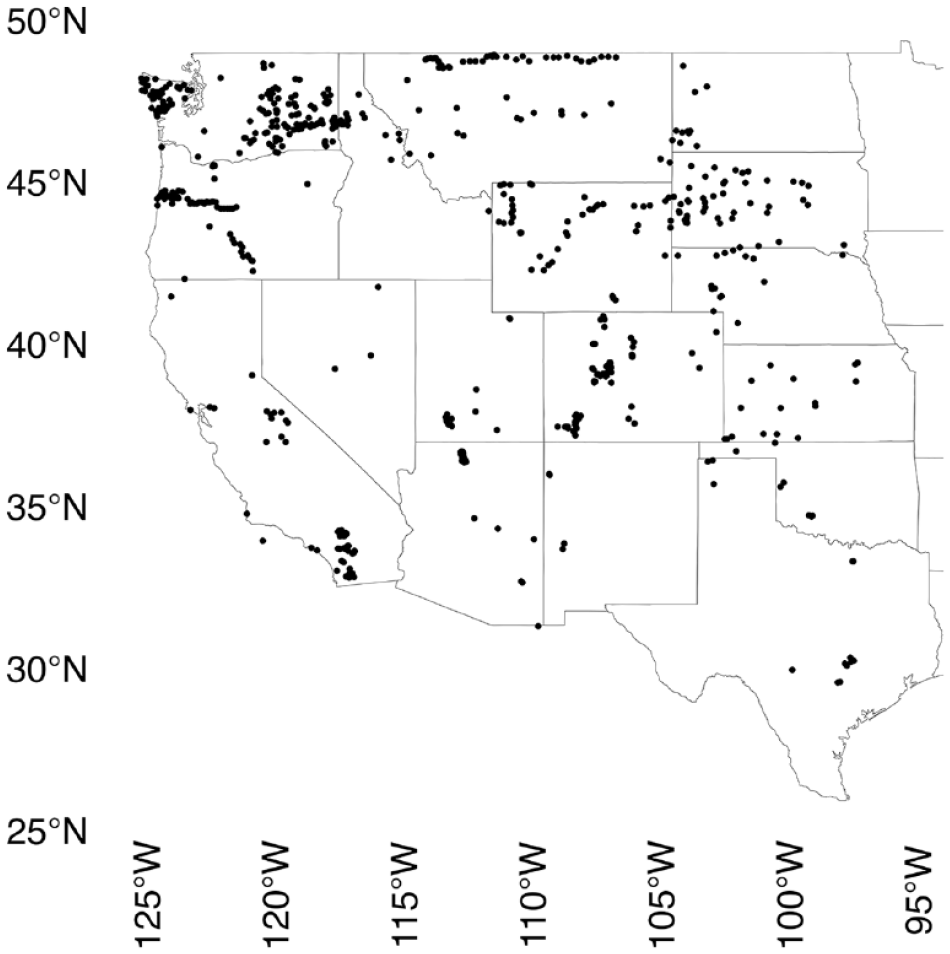
Modern pollen samples used in this study from the Neotoma Paleoecology Database.

Figure 2.

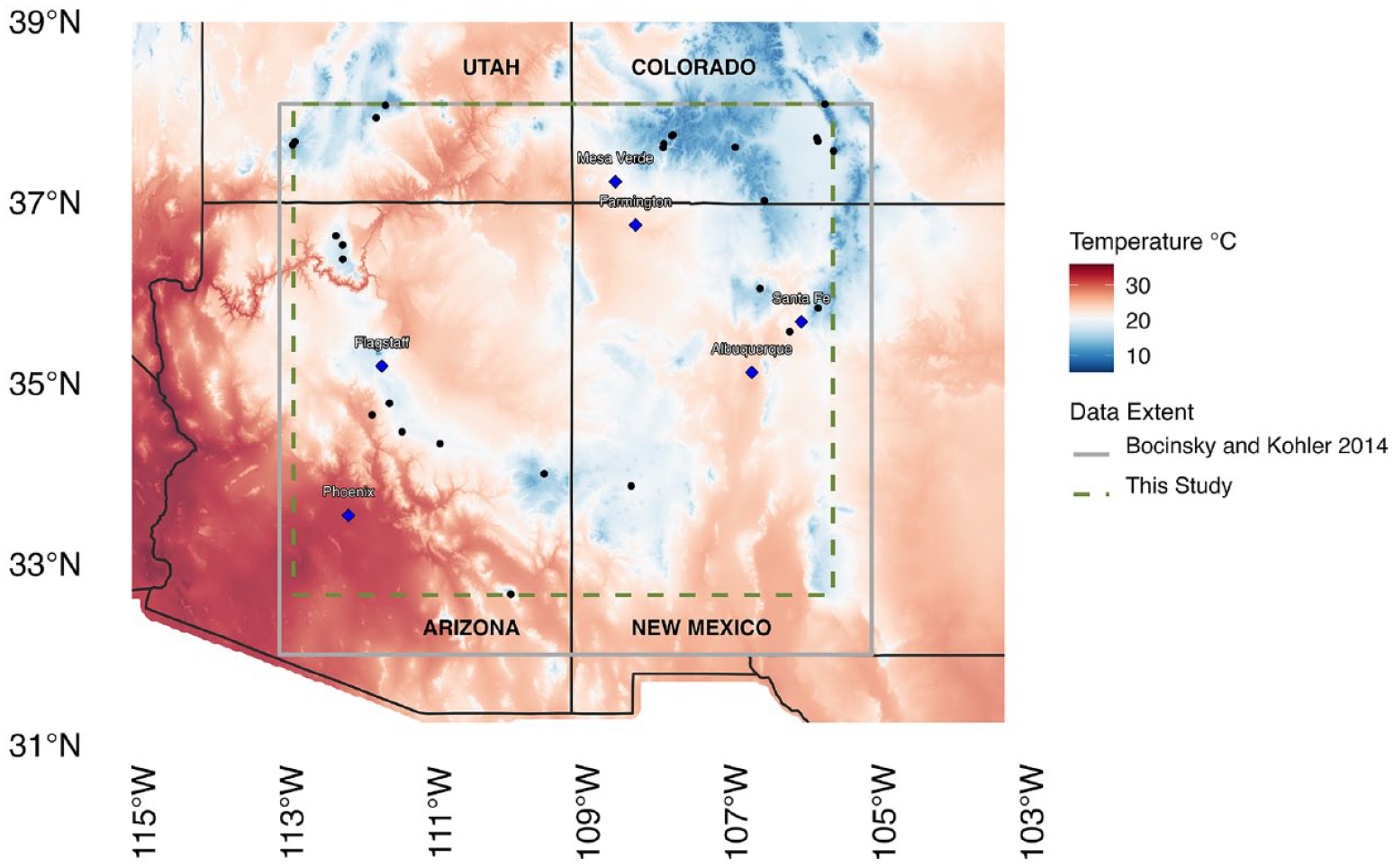
The Southwest United States (SWUS) as defined here, showing locations of fossil pollen samples used in this study. Background shading indicates mean July temperature for 1961–1990 from PRISM (Daly et al., 2008, 2015; PRISM Climate Group, 2019) at 800 m resolution. The solid gray box outlines the area studied by Bocinsky and Kohler (2014); the green dashed box shows the extent of the reconstruction in this study.

In the SWUS, climate reconstructions used by archeologists have been primarily based on tree-ring data. Although first used for relative dating (Douglass, 1929), tree-ring chronologies are used to reconstruct regional climates and create climate-field reconstructions which allow for calibration of variance across regions. Tree rings excel in storing and representing high-frequency (seasonal to decadal scale) climate signals in this area (Bocinsky et al., 2016; Dean et al., 1985), including for temperature. However, few tree-ring chronologies are available for this region before approximately AD 500 (Ahlstrom, 1997; Berry, 1982: 11; Bocinsky and Kohler, 2014). Moreover, it is difficult to extract a low-frequency (multi-decadal to millennial-scale) climate signal from tree-ring records (Cook et al., 1995). The temperature amplitudes in the low-frequency temperature data that are not present within the detrended high-frequency data would provide a more complete view of past climate, particularly the effects of large-scale climate patterns such as the El Niño/Southern Oscillation (ENSO) and the Pacific Decadal Oscillation (Cook et al., 1995; Dean, 1988, 1996; Dean et al., 1985; Fritts, 1991).

Possible pathways out of these difficulties are to employ large-scale pollen databases such as Neotoma Paleoecology Database (Williams et al., 2018) to do more comprehensive regional-scale pollen-based paleoclimate reconstructions through MAT (Overpeck et al., 1985; Whitmore et al., 2005; Williams and Shuman, 2008); to employ weighted averaging, or weighted-averaging partial-least squares regression (Chevalier et al., 2020) to well-dated fossil pollen assemblages; or to produce global-scale databases/analyses (Kaufman et al., 2020).

In this paper, we use MAT to reconstruct hottest month temperatures (July) for the past five millennia using pollen records for the SWUS – a period covering all of the time that maize has been grown in this region. We use the pollen data stored in the Neotoma Paleoecology Database, which incorporates the North American Pollen Database (Gajewski, 2008; Grimm, 2010; Grimm et al., 2007). These data have been widely used for climate reconstructions on multiple scales (Bartlein et al., 2011; Sawada et al., 2004; Viau et al., 2012; Williams et al., 2007; Wright, 1993). Our reconstruction benefits from new age-depth models in our sample.

Over the last few decades, paleoclimate reconstructions have greatly improved, as has our understanding of the effects of climate-driven variability on past societies (d’Alpoim Guedes et al., 2016; Jackson et al., 2022; Scheffer et al., 2021). Today, as climate change and our awareness of it accelerate (Masson-Delmotte et al., 2021), climate-change impacts to livelihoods and health of populations continue to grow (Hallegatte and Rozenberg, 2017; Rao et al., 2017; Shayegh, 2017). Paleoclimate reconstructions provide data to understand the dynamic mechanisms and responses of the earth’s climate system and its sensitivity to greenhouse gas concentrations (Mann, 2021); and the impacts of climate change on plant and animal communities (Crausbay et al., 2020; Fontúrbel et al., 2018), on biodiversity (Vicente-Serrano et al., 2020), and on human societies (Pörtner et al., 2022).

A brief history of Holocene temperature in North America

Ice core records and a collection of many temperature records provide general temperature trends for the Northern Hemisphere (NH) at a high temporal resolution. Figure 3 shows changes in temperature using the Greenland ice core data (Alley, 2000; Cuffey and Clow, 1997) and global mean surface temperature change (Osman et al., 2021) (using the 50th ensemble percentile) from 22,000 BC to the present (Alley, 2000). The Younger Dryas (YD) event (10,850–9550 BC or 12,800–11,500 cal BP) – a major cooling event following a very warm period (ca. 12,550 BC) – presents the largest and most rapid temperature change in the last 20,000 years. The YD seems to have brought cooler and wetter conditions to the SWUS (Huckleberry, 2015). Post-YD warming was followed by another cold event (albeit much less severe than the YD) around 6250 BC (Alley et al., 1997).

Figure 3.

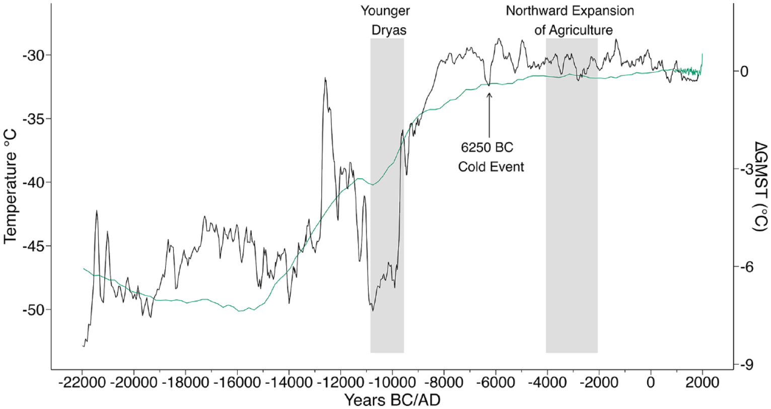
Temperature for the North Atlantic using Alley’s (2000) Greenland ice core data (black line) and global mean surface temperature change (Osman et al., 2021) (using the 50th ensemble percentile) for 22,000 BC to present with the Younger Dryas and the general period of the northward expansion of maize agriculture from Mesoamerica into the SWUS highlighted.

How these trends played out in North America (NA) over the last 12,000 years has been determined in part from the pollen record using MAT. Viau et al. (2006: 3–4) noted a “four-part division of the Holocene: a rapid warming of the early Holocene until circa 8000 cal. yr. BP [6050 BC], a cooling between 8000 cal. yr. BP [6050 BC] and 6000 cal. yr. BP [4050 BC], a warmer middle Holocene, and a late-Holocene cooling after 3000 cal. yr. BP [1050 BC].” Maize agriculture expanded northward from south-central Mexico between 5050 BC and 2050 BC, a period of relative warmth and climatic stability by this reconstruction. Around 4050 BC during the warmest month (July), the SWUS was slightly warmer, generally drier, and with more intense summer monsoons than at present (Bartlein et al., 1998; Mock and Brunelle-Daines, 1999). By 3050 BC, southwestern plant communities were generally similar to those of today in composition and location (Thompson and Anderson, 2000). At Chihuahueños Bog in the Jemez Mountains of northern New Mexico, Anderson et al. (2008a) date the arrival of the local modern mixed conifer forest to around 4450 BC. Four temperature peaks have been extrapolated from the Greenland ice core data to the post-2050 BC Southwest: at approximately 1350 BC, 120 BC, AD 435, and AD 985 (Alley, 2000; Huckleberry, 2015).

Within the last two millennia for the NH, Moberg et al. (2005) use multiple proxies to reconstruct a cool early first millenium AD, with temperatures increasing to a peak between AD 917 and 1106 during the MWP, followed by a marked decrease in temperature with a minimum around AD 1575 during the LIA (Figure 4). These main features are also visible in Viau et al. (2006) NA reconstruction. PAGES2k also reconstructed NH temperatures using many different proxies that combine high and low frequency data (Figure 4) (Neukom et al., 2019). A number of more recent NH temperature reconstructions are available for all or most of the last two millennia, including that of the N-TREND (Northern Tree-Ring Network Development) consortium for AD 750–1988 (Anchukaitis et al., 2017) and the multi-proxy reconstruction of Ljungqvist (2010) extending to AD 1.

Figure 4.

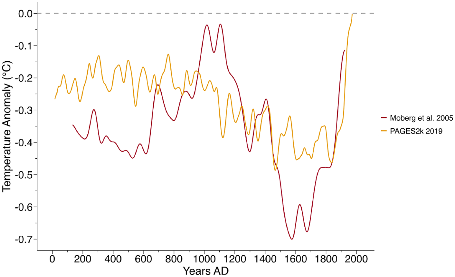
Low-frequency component of the Moberg et al. (2005) multi-proxy reconstruction for Northern Hemisphere for AD 133–1925. PAGES2k reconstructed NH temperatures using different proxies that primarily shows high frequency resolution (Neukom et al., 2019). Anomalies for both series are calculated in comparison to the 1961–1990 average.

Some NA temperature reconstructions are spatially explicit, permitting identification of variability specific to the US Southwest. Viau et al. (2012) include a MAT reconstruction for the Desert biome for NA in the last two millennia. The space they assign to this biome extends considerably in all directions beyond the SWUS as defined here, however. Using pollen as a proxy analyzed using MAT, their reconstruction begins at AD 1, shown as warmer than today (AD 1961–1990), with temperatures declining to a low of around -1 °C relative to today from AD 400 to 500, the coldest period in the last two millennia in this area, according to their reconstruction. Temperatures then increased, reaching a global peak around AD 900 with temperatures of about 1°C warmer than today (Viau et al., 2012). Relative temperature stability is reconstructed from about AD 1050 to 1450, with a small local peak around 1550 followed by a slight decline around AD 1600. Neither the MWP nor the LIA is strongly represented in their regional reconstruction.

Other studies have used one or two pollen cores to interpret temperature using pollen ratios (Petersen, 1988; Wright, 2006, 2010, 2012). For example, the Twin Lakes pollen core in southwestern Colorado suggested that first-millenium-AD temperatures were colder prior to AD 600 (Petersen, 1988). Wright (2010, 2012, 2006) estimated temperature and winter precipitation from a core at Beef Pasture (also in southwestern Colorado), which showed that from 100 BC to AD 600 temperatures and winter precipitation were low, after which they increased substantially.

Despite all this work, a few years ago Benson and colleagues identified problems with all the then-available proxies for temperature in the SWUS (including both tree rings and pollen), ranging from low correlation with instrumented temperature records (for high-altitude bristlecone pine) and questionable pollen ratios or low temporal resolution (for pollen) (Benson et al., 2013). Huckleberry (2015: 90) has also noted that temperature reconstructions for this region seem to be subject to contradictory interpretations. Here we address this challenge with a regional-scale approach based on fossil pollen.

Methods

We use pollen data to produce low-frequency temperature reconstructions using the MAT (Overpeck et al., 1985; Viau et al., 2006, 2012; Whitmore et al., 2005; Williams and Shuman, 2008) for the SWUS for 3000 BC–AD 2000. Our study area represents the smallest rectangle enclosing all the fossil pollen sites within the area modeled by Bocinsky and Kohler (2014), who produced a high-frequency climate-field reconstruction of the rain-fed maize agricultural niche for this area based on tree-rings (Figure 2).

Computer code

The computer code written in the R statistical language (R Core Team, 2021) for all analyses reported here is available as a R package, paleoMAT (Gillreath-Brown, 2023), for producing pollen–based paleotemperature reconstructions over the southwestern United States. All code for analysis and reconstruction is in “UUSS_MAT_Reconstruction.Rmd” and all code for figures and tables is in “Paleomat_Figures.Rmd,” which can be accessed at https://github.com/Archaeo-Programmer/paleomat. Other essential software packages used in this analysis include analog (Simpson, 2007) and palaeoSig (Telford, 2019), available at https://cran.r-project.org.

Data

We use the fossil and modern pollen data from the Neotoma Paleoecology Database (Williams et al., 2018) (data downloaded on October 23, 2021 using the neotoma 1.0 R package). Neotoma’s holdings are particularly comprehensive for fossil pollen samples in North America and Europe, though they are unevenly distributed across these areas. Currently, modern pollen samples in the database are almost exclusively limited to North America. For the SWUS, we use 29 fossil pollen core sites – 32 datasets with altogether 1478 samples that have dates via age models – within our study area (Table 1), which are (unsurprisingly) mostly in higher elevation areas (the colder areas shown in Figure 2). We exclude archeological samples (or sites that have complex human and animal influences, such as Bechan Cave) and other fossil pollen cores that do not have sufficient chronologies or do not contain data relevant to our study period of the last 5000 years (e.g. Black Mountain Lake, Dead Man Lake, Mayberry Well, and Sagehen Marsh). The mean elevation for the 29 fossil pollen sites is 2788 m with a minimum of 1112 m and maximum of 3701 m. We applied several quality control filters on the fossil and modern pollen dataset generally following (Chevalier et al., 2020): (1) minimum of 200 pollen grains identified in individual fossil samples, (2) assign 0 to observations with < 1% abundance, (3) remove taxa that occur in less than 20 samples, and (4) remove samples that have less than five unique taxa. Due to the low number of pollen samples in the western United States (when compared to the east), we used 200 grains as the minimum count (Chevalier et al., 2020). Twenty-nine sites (comprising 32 datasets and 773 samples [only 38 samples were removed by the quality control filters; 635 samples were removed because the max age was older than 6000 years cal BP, which we use as a buffer for beyond our study period to anchor the temperature curve]) with a mean elevation of 2788 m contain sediments dated to the period of interest here and pass the quality control filters. Data for each fossil pollen core includes depths, elevation, age models, pollen taxa, and pollen counts.

Table 1.

Metadata for the fossil pollen records (29 sites or 32 datasets) used in this study that have data after 3550 BC.

Site Name	Site ID	Dataset ID	No. of Samples	Elevation (m)	Longitude	Latitude	References
Alpine Pond	9814	14517	26	3028	−112.82446	37.63632	Anderson et al. (1999)
Alpine Pond	9814	14547	11	3028	−112.82446	37.63632	Anderson et al. (1999)
Bear Lake	10000	14951	12	2752	−112.14718	36.371125	Weng and Jackson (1999)
Beef Pasture	246	250	89	3076	−108.16038	37.473105	Petersen (1985); Petersen (1994); Petersen (1988)
Beef Pasture	246	25551	71	3076	−108.16038	37.473105	Wright (2006, 2012)
Cascade Fen [Engineer Mountain Bog]	339	347	63	2845	−107.80868	37.647645	Bender et al. (1966); Maher (1961), (1963)
Chihuahueños Bog	13680	20833	18	2862	−106.51053	36.047665	Anderson et al. (2008b)
Columbine Ranch Fen	486	498	28	2793	−107.81571	37.60664	Bender et al. (1967); Maher (1961), (1963)
Como Lake	2957	3056	9	3651	−105.51417	37.569525	Jodry et al. (1989); Shafer (1989)
Crane Lake	504	517	7	2664	−112.1489	36.52986	Shafer (1989)
Cumbres Bog	11617	17419	29	3115	−106.45052	37.021745	Johnson (2010); Johnson et al. (2011)
Fracas Lake	9997	14944	7	2530	−112.2386	36.6307	Weng and Jackson (1999)
Hay Lake	982	1013	5	2764	−109.425	34	Jacobs (1983), (1985)
Head Lake	2955	3054	9	2295	−105.74064	37.71109	Jodry et al. (1989); Shafer (1989)
Hermit Lake	23930	41580	26	3701	−105.63166	38.08806	Anderson et al. (2021)
Hospital Flat Meadow	26738	46801	9	2875	−109.87742	32.66757	Anderson and Smith (2009)
Hunters Lake	13486	20304	20	3576	−106.8437	37.611035	Anderson et al. (2008a)
Jacob Lake	1127	1162	5	2326	−110.83333	34.333333	Jacobs (1983)
Leonora Curtin	14632	22948	12	1867	−106.10652	35.56948	Edwards (2015)
Lowder Creek Bog	9830	14549	12	3186	−112.79225	37.67214	Anderson et al. (1999)
Molas Lake	1705	1761	25	3282	−107.68274	37.74759	Carrara (2011); Maher (1972); Maher (1961); Stuiver (1969)
Molas Pass Bog	1706	1762	15	3362	−107.6975	37.737778	Bender et al. (1970); Hubbs et al. (1963); Maher (1972); Maher (1961), (1963)
Montezuma Well	1710	1766	31	1112	−111.75225	34.6492	Davis and Shafer (1992); Shafer (1989)
Posy Lake	1905	1970	14	2693	−111.69604	37.93746	Shafer (1989)
Potato Lake	1906	3560	14	2280	−111.34528	34.462222	Anderson (1989, 1993); Anderson et al. (1989); Whiteside (1965)
Potato Lake	1906	3561	15	2280	−111.34528	34.462222	Anderson (1989, 1993); Anderson et al. (1989); Whiteside (1965)
Purple Lake	13683	20838	39	3321	−111.57115	38.07438	Morris et al. (2013); Morris and Brunelle (2012)
San Agustin Plains	2260	3612	5	2115	−108.25	33.866667	Markgraf et al. (1984)
San Luis Lake	9878	14650	20	2295	−105.72467	37.67773	Jeanne Lusielle (1993)
Stewart Bog	10191	15356	101	3083	−105.722	35.832	Jiménez-Moreno et al. (2008)
Stoneman Lake	10449	15967	17	2132	−111.51778	34.778865	Hasbargen (1993, 1994)
Twin Lakes	2785	2880	54	3265	−108.10256	37.46906	Petersen et al. (1985); Kenneth Lee Petersen, (1994); Petersen and Mehringer (1976)

All data were downloaded from the Neotoma Paleoecology Database (Williams et al., 2018).

All 32 cores have Bacon age-depth models, which use the IntCal20 calibration curve (Reimer et al., 2020); these are Bayesian age models available in R using the rbacon package (Blaauw and Christen, 2011). After construction of the age-depth models, all dates are in calendar years. We provide the chronological control points, Bacon parameter settings, and the output files for each pollen core from Bacon in the GitHub repository. Supplemental Figure S5 shows a histogram for the fossil pollen samples using the median date for each sample in 100-year bins. The number of samples is lower prior to approximately 2000 BC, which shows temperature changes over longer time scales than later in the series. Each core has chronological uncertainty due to radiocarbon dating density and quality and the dating method (e.g. conventional radiometric and accelerator mass spectrometry 14C dating) (Blois et al., 2011). Each pollen sample has an age range in calibrated years that is provided by the age-depth model. In some cases, the range may be relatively small (e.g. 50 years), but can be larger in other cases (e.g. 300 years). A larger uncertainty range could reflect vegetation changes over multiple centuries. For example, if we were to simply use a mean date for a fossil sample, then the vegetation change would only be reflected in one century rather than in three centuries. Therefore, to account for the chronological uncertainty, we rebuild the age-depth model 100 times for each record. Then, we rebuild the synthesis temperature curve repeatedly (i.e. 100 times) from the different distribution of samples in time.

For the modern pollen samples, we limit the calibration dataset (i.e. the modern pollen data) to the western United States, as defined by the maximum extent of western species listed in Williams and Shuman (2008) supplementary data (i.e. the western shapefiles). Williams and Shuman (2008) argue that limiting samples in this way improves MAT precision and accuracy. The western United States has 765 modern pollen samples (Figure 1). We applied the same quality control filters that were used for the fossil pollen dataset to the modern pollen dataset, which yielded 646 samples. Similar to the fossil pollen samples, the modern pollen samples are sparse and unevenly distributed across the study area. To assign climate parameters to these modern pollen samples, we use contemporary weather data from the Parameter Elevation Regression on Independent Slopes Model (PRISM) (Daly et al., 2008, 2015; PRISM Climate Group, 2019), which includes monthly temperature (i.e. minimum, maximum, and mean) modeled at an approximately 800 m scale. To each modern pollen sample, we assign the mean July temperature for its PRISM cell averaged for the 30 years from 1961 to 1990.

We are unable to compare our sample coverage for the fossil pollen sites with that of Viau et al. (2012, Figure 3) for their Desert biome – the only previous published application of MAT to the SWUS as a whole (as opposed to single pollen core studies (e.g. Davis and Shafer, 1992) – since they did not provide a table listing how they spatially subset the 748 pollen records then available through the North American Pollen Database. However, it is likely that they were unable to include several cores included in our sample due to their recency (Beef Pasture (Wright, 2012); Cumbres Bog (Johnson, 2010); Leonora Curtin and La Cienega (Edwards, 2015); and Purple Lake and Aquarius Plateau (Morris et al., 2013)). On the other hand, they presumably included a number of fossil pollen sites within the Desert biome but beyond the limits of our study area.

Modern analog technique

In general, vegetation on a large scale responds to variability in temperature and precipitation with a lag, roughly considered to be in the 50–100-year range when examining pollen records (Bertrand et al., 2011; Corlett and Westcott, 2013; Harrison and Sanchez Goñi, 2010; Svenning and Sandel, 2013; Thom et al., 2017; Williams et al., 2021). However, with rapid and persistent climate changes, vegetation may respond more quickly than 50–100 years (Tinner and Lotter, 2001), although this is usually less apparent in the pollen record. MAT employs modern pollen/climate correlations to reconstruct past temperatures from fossil pollen data, assuming that past climate variability will affect the same changes in vegetation composition as contemporary climate variability.

MAT relies on a dataset of modern pollen samples paired with modern temperatures, here derived from PRISM. Fossil pollen assemblages are matched to particular similar modern pollen assemblages – their “analogs” – through a dissimilarity measure such as the squared-chord distance (SCD) we use here (Overpeck et al., 1985). Typically, in uses of the MAT, several modern analogs each with its own associated local temperature are averaged for each temperature estimate, so that local anomalies or disturbances have reduced effects on the overall climate series. The exact number to use has been the subject of much discussion (Williams and Shuman, 2008).

For determining the best fossil pollen samples and sites to use in our reconstruction, we use several transfer function and reconstruction diagnostics, such as squared residual length, the proportion of variance in the fossil data explained by an environmental reconstruction, and the no-analog threshold. These diagnostics are used to avoid poor reconstructions. First, we fit the fossil data passively onto the first axis of an ordination of the modern calibration data (Birks et al., 1990; Birks et al., 2010; Telford, 2014a). This goodness-of-fit test is used to determine whether an individual fossil sample fits onto the axis by using the squared residual length. The modern calibration set is constrained by the single environmental variable we are reconstructing (July temperature). Observations within the assemblage that are well explained by the variable will be close to the first axis. Fossil samples with a large squared residual length in comparison to the distribution of squared residual lengths of the modern calibration data (we use greater than 95% of the lengths) are poorly fitted by July temperature. By removing the poorly fitted samples from the dataset, we reduce some uncertainties in the data. We used the residLen function in the analog package to calculate the squared residual length (Simpson, 2007; Simpson and Oksanen, 2021). Using this test, we removed 51 of our 773 samples (leaving 28 sites, 31 datasets, and 722 samples) (Supplemental Figure S1).

Then, using this smaller set of data which was assured to be of high quality for our purposes, we used functions in the analog package (Simpson, 2007; Simpson and Oksanen, 2021) to define the transfer function from the modern pollen and temperature data, and to make temperature predictions for the fossil pollen assemblages (i.e. to reconstruct the mean temperature of the warmest month, July). We used the SCD to identify the four best (least dissimilar) modern pollen samples to serve as analogs for the temperature under which a particular target fossil pollen sample was formed. The optimal value for k can be determined using a root mean squared error of prediction (RMSEP), which are leave-one-out errors for the training set (Supplemental Figure S2). The prediction for each sample in the modern training set is based on the k-closest analogs excluding that particular sample (Simpson, 2007). Supplemental Figure S2 shows the values for leave-one-out errors (RMSEP); we use k = 4, which has the lowest RMSEP value (Supplemental Table S1). Williams and Shuman (2008: 684) argue that “multiple matches per sample reduces stochasticity and improves precision.” We averaged the PRISM-derived interpolations for the July temperatures from 1961 to 1990 at each modern pollen sample site to determine the best July temperature estimate for each sample from each fossil pollen core. Spatial autocorrelation in the modern dataset can bias transfer function estimates (Guiot and de Vernal, 2011; Juggins and Birks, 2012; Telford and Birks, 2009; Trachsel and Telford, 2016). When an environmental variable is spatially autocorrelated, then species assemblages that are spatially close tend to be similar. Therefore, MAT tends to overestimate values due to geographical reasons. However, one way to remove the influence of spatial autocorrelation is to use h-block cross-validation to get unbiased transfer function estimates. For the reconstruction, we exclude samples within 300 km of a target site to minimize the effects of spatial autocorrelation.

Finally, we apply a non-analog threshold to reconstructed samples using the minDC function from the analog package (Chevalier et al., 2020; Simpson, 2007; Simpson and Oksanen, 2021; Telford, 2014b; Williams and Shuman, 2008). The minDC function returns the minimum dissimilarity for each predicted sample (i.e. between a fossil pollen sample and the modern training samples). If there are no close modern analogs in the modern samples for a fossil pollen sample, then we cannot reliably make an environmental inference for that sample. For the no-analog threshold, we use the fifth percentile of the pair-wise distribution of the SCDs for the modern calibration set (Jackson and Williams, 2004; Simpson, 2012; Telford, 2014b) (Supplemental Figure S3). The fifth percentile value can be acquired from the output of the transfer function model (i.e. the output of the mat function). So, samples that have distances shorter than the fifth percentile represent good analogs. Using the fifth percentile, we removed 173 samples that did not have good analogs (leaving 27 sites, 30 datasets, and 548 samples).

One open issue in MAT-based studies is how many and which taxa to use in computing the SCD. We used the 135-taxon list from Williams and Shuman (2008) (see also Whitmore et al., 2005) to assess the similarity among fossil and modern pollen samples. Our choice to use this larger list of taxa is another difference between this study and that of Viau et al. (2012: 377) who used a 63-taxa pollen sum. Williams and Shuman (2008: 683) argue that the “precision gains between the 135-taxon and 64-taxon lists are small to negligible.” However, we only use taxa that occur both in the modern calibration dataset and the fossil data (Chevalier et al., 2020). After applying the quality control filters to the pollen samples and only keeping overlapping taxa between the calibrated dataset and the fossil pollen dataset, we use 27 unique taxa for the reconstruction step.

Defining anomalies

Once the mean temperature of the warmest month has been estimated for each sample, we derive an estimate of how much that differs from modern conditions (the temperature anomaly). We calculate the anomalies at each fossil pollen core by extracting the modern average temperature from the PRISM data (i.e. mean temperature in July from 1961–1990) at the location of each core. We assume that anomalies of the same magnitude and sign apply to those portions of our study area without fossil pollen cores.

Moreover, instead of using the raw anomalies for each sample, we used a technique from the R package analog to calculate an estimate using bootstrapping (n = 1000) (Simpson, 2007). Bootstrapping is a method by which a random set of samples in the training set is replaced by samples of the same size, where some observations are used multiple times and some samples will not be used at all (Birks, 2014; Birks et al., 1990; Birks and Simpson, 2013; Efron, 1982; Freedman, 1981; Herbert and Harrison, 2016; Simpson, 2007). These bootstrapped anomalies are very similar to those produced in the traditional manner, as shown in Supplemental Figure S4 (see also Supplemental Table S1); the linear correlation between the two series as measured by r² = 0.96 (p > F < 0.001). One advantage of bootstrapping is that it provides a measure of sample-specific errors, which we examine below.

Time series: Boxplots and loess curves

We present aspects of our results in three different ways. At the highest resolution, the averaged bootstrapped temperature anomaly estimates for each retained sample from each fossil pollen core are shown in Figure 5 as small circles, which are plotted on the median date for each sample. The sizes of the circles representing each sample are inversely proportional to the bootstrap sample-specific errors for each sample (see Simpson, 2007: 21 for calculation); anomaly estimates with larger circles can be viewed as more precise (Supplemental Table S1).

Figure 5.

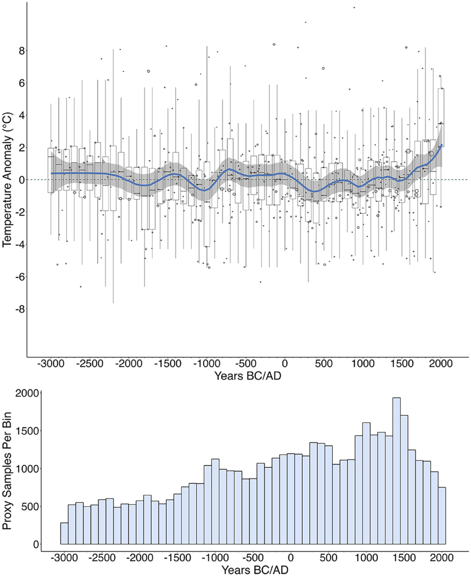
Low-frequency bootstrapped summer temperature anomaly loess reconstruction from this study (blue) with standard error (gray) (top figure). Boxplots show estimates binned by century for all proxy samples (i.e. includes samples for the 100 simulations of the age-depth models). Anomalies are calculated in comparison to the 1961–1990 average. The temperature predictions using the median date from the age-depth model (i.e. does not include the 100 simulations) for each sample (not binned by century) are shown by circles; sizes of circles are inversely proportional to the sample-specific errors (size of circle ∝ 1/s1; see Simpson, 2007: 21 for calculation of s1). Anomaly estimates with larger circles are more precise. Histogram of proxy samples that includes the 100 simulations of the age-depth models through time in 100 years bins.

As these individual estimates show, even after filtering to remove samples/cores with little temperature information or no analogs, MAT can produce a noisy reconstruction. The remedy for this is not prior pooling of data: as shown by Herbert and Harrison (2016), individual samples should be reconstructed first before their mutual patterning is sought out (as we have done here and is common practice) rather than pooling samples together then reconstructing. We use two main techniques to extract a signal from this noise, both of which feature robust statistics. First, we apply a loess smoother (superimposed on the sample data in Figure 5), which is relatively insensitive to outliers, and which does not begin by specification of a function (Cleveland, 1979). After experimenting with various spans (α) we settled on 0.15 as presenting the best compromise between rough and smooth. In our 5000-year dataset, this results in a moving window that is on average 750 years wide within which datapoints are weighted within the neighborhood of year according to a tri-cubic function dictating that influence of years declines rapidly as one moves away from the current target. Within that window, and with those weights, a second-order polynomial least-squares function is fitted to determine the temperature anomaly for each year. The confidence interval plotted around the loess curve is the standard error of the estimate for the temperature anomaly at that date. The loess curve in Figure 5 is not weighted by the inverse of the bootstrapped errors shown in the circle sizes; in Supplemental Figure S6 we present an alternative version that is so weighted. The two curves are very similar, with the most apparent difference being slightly cooler around 1000 BC in the weighted version.

Any smoother, by definition, throws out detail to provide a simple approximation to the data. To present the raw data in a higher-resolution form than the loess curve, we employ box-and-whisker plots by century along the loess curve (also in Figure 5). These box plots summarize the raw data at what we consider to be their maximum-usable temporal resolution (one century) using the most robust temperature-anomaly estimate at that temporal scale (the median). We use common conventions for these boxplots (Tukey, 1977): the mid-point of the distribution is represented as a line at the median; the upper and lower limits of the interquartile range (IQR) are plotted as the top and bottom of the box, respectively; and the whiskers extend to the largest(smallest) values within 1.5 times the IQR. Here though we do not display individual values beyond the whiskers as part of the boxplots, since all the individual values are already shown, and at a higher temporal resolution. In those portions of the curve where samples are most numerous (the last 1500 years) the loess curve usually passes through the century medians, though it is not constrained to do so. Rapid changes in temperature, or lower density of sampling, will sometimes cause divergence between the loess curve and the century medians, as is common in the first two millennia of this reconstruction. The confidence band around the loess curve encloses or intercepts the boxplot medians in 84% of the centuries; all the exceptions are in the first 2000 years of the reconstruction. Below we present our results with primary reliance on the loess curve, referring to the higher resolution boxplots in the Discussion.

Results

The July temperature anomalies reconstructed here show fluctuating summer temperatures in the SWUS for the five millennia (Figure 5). During the third millenium BC, 1400 BC, 700–1 BC, AD 750, and AD 1100–1200 (prior to AD 1800), loess-modeled summer temperatures slightly exceeded or were close to those of the modern period.

Following a warm third millenium BC, summer temperatures dipped below modern from about 1900 to 1600 BC and from about 1200 to 900 BC. We reconstruct a 500-year period in which SWUS summers were cooled, beginning around AD 1 until AD 500 with the global minimum in this reconstruction around AD 400. After that summer temperatures generally increased until around AD 1400, punctuated by marked cooling around AD 900 and again (less markedly) around AD 1500. The LIA is expressed only faintly in this record as two centuries with cooler summers around AD 1400–1500, after which summer temperatures rapidly increased. The final increase in our reconstruction beginning around AD 1850 is in line with numerous other reconstructions based on various proxies as well as instrumented data but should still be treated with caution given vegetative disturbances by Euro-American industry by that date, possibly affecting the pollen rain on which the MAT depends. Taken at face value, however, our reconstruction shows that the rapid warming beginning in the 1800s is unprecedented in the US Southwest in at least the last five millennia.

Discussion

The period covered in our reconstruction includes both the “Subboreal” and the “Subatlantic” as these terms are traditionally applied in Europe, and the “Neoglacial” as the late-Holocene is sometimes called in North America. In comparison with the early and middle Holocene, this third phase of the Holocene is dominated by declining summer insolation in the NH (Wanner et al., 2008). This caused a general global trend of declining temperatures in the late-Holocene as shown in Figure 6 in which we reproduce composite terrestrial temperature anomaly estimates for the 30–60ºN latitudinal band from Kaufman et al. (2020, Figure 6).

Figure 6.

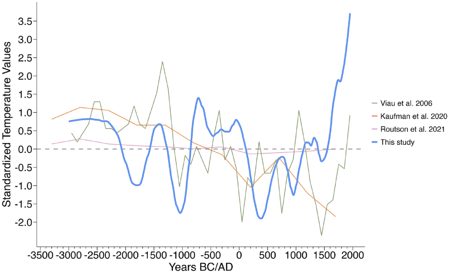
Low-frequency July temperature anomaly for the SWUS from this study, the North American July temperature reconstruction (Viau et al., 2006) from 3000 BC to AD 2000, the terrestrial composite for 30–60°N (Kaufman et al., 2020) from 3300 BC to AD 1700 in 500-year bins, and summer temperature for western North American (Routson et al., 2021). All series standardized to a mean of 0 and an s of 1 over the period in this graph (Routson et al., 2021 was already standardized).

ENSO

The declining temperatures in the late-Holocene in turn caused the summer position of the Intertropical Convergence Zone to drift to the south. Wanner et al. (2008) suggest that these changes in turn led to increasing amplitude of the El Niño/Southern Oscillation (ENSO). “The ENSO phenomenon represents the most important branch of internal variability of the global climate system” (Wanner et al., 2008: 1808) and “the Earth’s strongest source of year-to-year climate variability” (Santoso et al., 2017: 1079). Positive values (La Niña-like conditions) are strongly linked to droughts and warm temperatures in the SWUS whereas El Niño-like conditions are associated in the SWUS with high precipitation (Cook et al., 2014; Mann, 2021) and cool conditions. World-wide, higher temperatures are generally associated with higher precipitation (Marcott et al., 2013: 1199), but for at least portions of the upland SWUS, high annual (tree-ring) temperatures tend to accompany dry conditions (Dean and Van West, 2002). In general, ENSO activity has been difficult to understand for the last 5000 years with multiple conflicting records (Huckleberry, 2015). “La Niña-like” conditions may be responsible for extended drought conditions, with additional linkages to temperature variability across the SWUS (Bale et al., 2011).

Although ENSO mean state and variability affect many portions of the world, including the Pacific Northwest, South America, Africa, Australia, and Indonesia (Mann, 2021), their effects on the SWUS and the western portions of Mexico, Central America, and northern South America are particularly direct. When the average temperature anomaly for the SWUS is relatively larger (warmer) than reconstructions for general NA or the NH, one cause could be a dominance of La Niña-like conditions differentially affecting the SWUS – particularly in comparison to larger-scale reconstructions not dominated by records that are highly sensitive to ENSO variability (Huckleberry, 2015). On the other hand, periods when the SWUS exhibits average summer temperature anomalies cooler than these benchmarks may suggest the dominance of El Niño-like conditions. The mechanisms that can lead to persistence of one ENSO state are not well understood. Recently Ding et al. (2022) have suggested that interactions with the North Pacific Oscillation can lead to multi-year El Niño events.

The longest high-resolution proxy for El Niño activity currently available, a sediment core off the coast of Peru spanning the last 20,000 years (Rein et al., 2005), suggests strengthening El Niño activity during this period. According to their main proxy, which is problematic for the Middle Holocene, El Niño activity generally increased from a 4000 BC low to a strong peak between about AD 200 and 1100. Following a relatively low period between about AD 1100 and 1500, this core reveals a burst of activity in the 1600s followed by a decline into the modern period.

Another remarkable proxy for El Niño activity comes from a high-elevation lake in Southern Ecuador (Moy et al., 2002). To simplify, this record shows low El Niño activity in the early Holocene, a prominent spike shortly after 3000 BC, low activity for a millenium centered on 2000 BC, two large spikes around AD 250 and 500, a distinct lull in activity around AD 1000, and a final (somewhat lower) peak around 1250, followed by a sharp decline (Moy et al., 2002, Figure 1a). Some caution in interpretation is necessary due to the possible influences of both Atlantic and Pacific water vapor sources, and regional inputs to large-scale controls on extreme precipitation events in this and other Andean lake cores (Sandweiss et al., 2020: 4). However, Andrea Brunelle found this proxy useful for predicting fire frequency in low-elevation ciénegas near the southern boundary of our study area, arguing that El Niños brought winter precipitation to this area, necessary to support vegetation growth and desert fire (Brunelle, 2022).

Attempts to reconstruct ENSO activity from archeological proxies in coastal Peru date back to the 1980s and rely on interpreting and dating stratigraphic events, on biogeography, and on the geochemistry of midden constituents such as marine mollusk valves and fish otoliths. Using these proxies Sandweiss et al. (2020) reconstruct El Niño frequency as low in the Middle Holocene, becoming much more frequent around 1000 BC and beginning to take on its contemporary periodicity thereafter.

Before common era

The warm third millenium BC (3000–2100 BC) in this new reconstruction is similar to the more general NA conditions reconstructed by Viau et al. (2006, Figure 2), who also found generally warm conditions from 4050 to 1050 BC (Figure 6). However, the third millenium BC as reconstructed here is cooler than the global terrestrial norm for this latitude likewise plotted in Figure 6. This may be attributable to a large peak in frequency of El Niño activity visible in the Laguna Pallcacocha core from ~3000 to 2500 BC (Moy et al., 2002, Figure 1a).

From 2000 to 1500 BC, our SWUS estimates are generally cooler than those from NA and the NH depicted in Figure 6, perhaps due to the infrequency of El Niño events in this period, but frequency of such events slowly accelerated between ~1000 BC and AD 1, before accelerating rapidly between ~AD 100 and AD 500 (Moy et al., 2002, Figure 1a), leading to the coolest summers in our record. During this period the relationship of the SWUS reconstruction with the continental and hemispheric is somewhat mixed except for the centuries from ~900 BC – AD 1 when the SWUS is relatively warmer than its comparators (Figure 6).

The last 2000 years

Considerable support is found for the very cool summer temperatures that we find already prevalent by shortly after the BC/AD transition. Moberg et al. (2005) reconstruct below-modern temperatures for the entire first millenium AD in the NH with a minimum (within this millenium) around AD 500 (Figure 4). The (Neukom et al., 2019) reconstruction in this figure primarily shows high-frequency variability (around multi-decadal scales), and thus the low-frequency may be underestimated, which is likely why their reconstruction diverges from that of Moberg. In their multi-proxy reconstruction for the extra-tropical NH, Ljungqvist (2010) also reconstruct lower-than-modern temperatures from about AD 200 to 980 with quite cold conditions from about AD 300 to 550.

We call attention to the interesting relationship between our SWUS temperature model and the NH reconstruction of Moberg et al. (2005). Figure 7 compares the summer temperature reconstruction from this study and Moberg’s NH low-frequency reconstruction (which contains proxies for spring, summer, winter and annual temperature) after standardizing both series to a mean of 0 and s of 1. Our temperature reconstruction is relatively cooler than that of Moberg for nearly the entire AD ~100 (when the Moberg reconstruction begins) to 1200 period, after which our reconstruction is consistently relatively warmer than that of Moberg. The same is true of the PAGES2k Consortium (Neukom et al., 2019) reconstruction (after standardizing), although theirs becomes cooler than ours at approximately AD 1100 rather than AD 1200. This could be explained by a dominance of El Niño-like conditions between AD 100 and 1200, and a dominance of La Niña-like conditions thereafter (until at least AD 1900). This is because our reconstruction, local to the SWUS, is much more affected by the ENSO phase than are these general NH reconstructions. However, z-scores for our reconstruction and that of Moberg are similar for AD 100–200, the early AD 600s, and from about AD 1250 to 1450, possibly suggesting reduced ENSO amplitudes in these periods. Moy et al. (2002, Figure 1a) graph three very strong peaks of El Niño activity at AD ~200–400, ~550–900, and AD ~1050–1200, after which frequencies rapidly decline in an almost linear fashion into the modern period. Figure 6 shows that our SWUS reconstruction is considerably cooler than NA and NH norms during the first two of these periods. From 1050–1200, our reconstruction is similar to Viau’s NA reconstruction and Routson et al.’s (2021) western North America reconstruction but warmer than Kaufman’s NH estimate. Figure 7 shows that of the three periods with strong El Niño activity according to (Moy et al., 2002), the first two were relatively much cooler in the SWUS than in the NH reconstruction of Moberg et al. (2005) and PAGES2k (2019), whereas the period from 1050 to 1200 is mostly slightly warmer than in PAGES2k.

Figure 7.

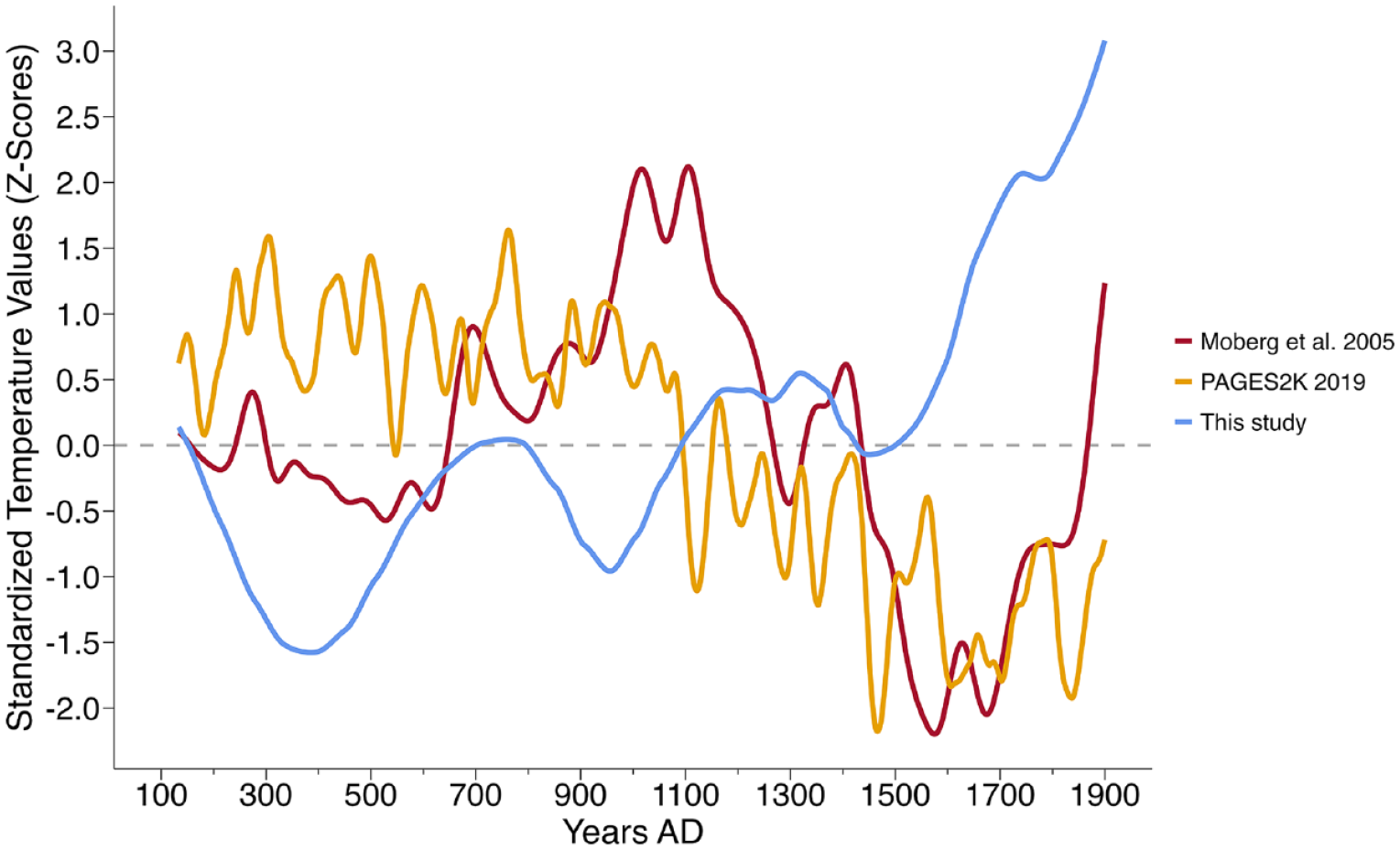
Low-frequency July temperature anomaly for the SWUS from this study and the Northern Hemisphere low-frequency component (Moberg et al., 2005) from AD 133 to 1900. PAGES2k reconstructed NH temperatures using different proxies that combine high and low frequency data (Neukom et al., 2019). All series have been standardized to a mean of 0 and an s of 1 for this period.

MWP

Two periods of traditional climate interest for southwestern archeologists are the MWP (eleventh to fourteenth centuries AD) and the LIA (fifteenth to nineteenth centuries AD) (Mann, 2021), periods of generally warmer and cooler conditions, respectively (Mann et al., 2009). In our temperature reconstruction, we see a warm peak at AD ~1100–1300, which is during the Medieval megadrought interval (AD 1100–1300) (Cook et al., 2015), but the following two centuries experienced slightly cooler summers. (AD ~1000 is also a temperature peak in the NH reconstruction by Moberg et al. (2005), and Ljungqvist (2010), among others). Soil moisture was low during the Medieval megadrought (Gillreath-Brown et al., 2019). We conclude that although the MWP in the SWUS contains some low-frequency warm temperatures, including two SWUS megadroughts in the mid-1100s and late 1200s (Williams et al., 2020), it is particularly distinctive in our low-frequency temperature reconstruction. The MWP, however, was critical in another sense that it marked the termination – for the moment at least – of the dominance of El Niño-like conditions that resulted in cool summer temperatures in the SWUS for much of the first millenium AD. Fossil coral records indicate a century of low ENSO variability in the MWP, suggesting that such periods can last far longer than seen in modern observations (Lawman et al., 2020).

LIA

Given the slightly cool 15th and 16th centuries in this record, the LIA constituted a marked, but temporary, halt in strong movement toward increasing summer warmth since a nadir near AD 900. Summer temperatures declined most noticeably from about 1350 to 1550. We suggest that the increasing dominance of La Niña-like conditions after about 1400 (suggested by the increasing positive divergence of our record from those of Moberg and PAGES2k) prevented the LIA in the SWUS from becoming as cold as some other areas (e.g. Europe). Note that the nadir in the Moberg NH series for the last two millennia is reached at AD ~1550, a time at which our reconstruction for the SWUS is increasing rapidly. In our series on the other hand, the five-millenium minimum is reached around AD 400 when El Niño-like conditions were dominant.

Implications

We will consider the implications of this reconstruction for prehispanic farmers in the SWUS in detail elsewhere. Here we simply note that it is dangerous to assume that NH- or even NA-specific temperature reconstructions will fit the SWUS. Although this new reconstruction does echo some common NH and NA patterns in its 1500-year-long decline to cold summers AD ~400 (Figure 6); its warm peak ca. AD 1100, and a local minimum during the LIA ca. 1500, other features (such as its global minimum AD ~400 and its local temperature maximum AD ~1100–1300) are more idiosyncratic. The pattern of these deviations, relative to Moberg’s low-frequency NH reconstruction for example (Figure 7), suggests that the temperature history of this area is more affected by the phase and intensity of ENSO than are comparable NH or NA records.

To say that a particular mode of ENSO was dominant in a particular era does not mean there were no exceptions. For example, using bristlecone pine ring-widths Routson and colleagues reconstruct a severe warm drought in the Rio Grande headwaters (within our study area) in the second century AD (Routson et al., 2011; Vierra and Vint, 2022). This is a period in which we suggest that cool, wet, El Niño-influenced conditions were dominant. And so they were, with a downward trajectory in our loess curve and boxplot can be observed in the 2nd-century AD (Figure 5). However, in keeping with the characteristics of the proxy used, we have aimed to identify broad tendencies rather than high-frequency events. The nature of the relationship between La Niña-dominated periods and megadroughts (Lin et al., 2022; Williams et al., 2022) in the SWUS remains an area of promising research.

Conclusions

We provide a new low-frequency summer temperature history over the last five millennia for a portion of the Southwest US heavily populated long before the arrival of European conquistadors, and today. The reconstruction generated here reveals patterns in late-Holocene summer temperature trajectories in the US Southwest that could not be recovered from individual fossil pollen sites or by analysis of tree rings. This reconstruction differs in some respects from continental and hemispheric temperature reconstructions for the same period.

We find a warm third millenium BC and a second millenium BC in which summer temperatures were cooling at the beginning and end of the millenium. These are followed by a rather sharp dip around 1000 BC, then a mostly warm early first millenium BC that is followed by a millenium, beginning around 500 BC, in which summer temperatures gradually declined, reaching the global minimum in this reconstruction around AD 400. Thereafter, summer temperatures generally increased up to and including the AD 1100–1300 period (the MWP), punctuated by marked cooling in the AD 900s and AD ~1400s. The LIA is expressed in this record as a cool period from about AD 1400 to 1600, after which summer temperatures rapidly increased, in line with numerous other reconstructions based on various proxies as well as instrumented data. We argue that a major source of difference between this new reconstruction and others for North America or the northern hemisphere more generally is due to the more direct effect of ENSO phase and intensity on the Southwest US. To over-generalize a bit, frequent El Niño events suppressed summer temperatures relative to those in the northern hemisphere for much of the second millenium BC and from AD 100 to AD ~1100. In other periods, either ENSO was reduced in amplitude, or within a neutral phase, or La Niña conditions became dominant, boosting summer temperatures in the US Southwest relative to north hemisphere norms.

Supplemental Material

sj-docx-1-hol-10.1177_09596836231219482 – Supplemental material for A low-frequency summer temperature reconstruction for the United States Southwest, 3000 BC–AD 2000

Supplemental material, sj-docx-1-hol-10.1177_09596836231219482 for A low-frequency summer temperature reconstruction for the United States Southwest, 3000 BC–AD 2000 by Andrew Gillreath-Brown, R Kyle Bocinsky and Timothy A Kohler in The Holocene

Footnotes

Acknowledgements

We gratefully acknowledge the long and careful work of the dozens of palynologists who recovered and analyzed the records employed in this reconstruction. We also thank Eric Grimm, who updated age models for many of the fossil pollen cores used here. We were deeply saddened by Dr. Grimm’s passing on November 15th, 2020. Data were obtained from the Neotoma Paleoecology Database () on October 23, 2021, and its constituent database(s) (North American Pollen Database). The work of data contributors, data stewards, and the Neotoma community is gratefully acknowledged. We thank the two anonymous reviewers for their valuable, thoughtful, and constructive comments that helped to strengthen this paper.

Funding

The author(s) disclosed receipt of the following financial support for the research, authorship, and/or publication of this article: This material is based upon work supported by the National Science Foundation under Grants SMA-1637171 and SMA-1620462, and by the Office of the Chancellor, Washington State University-Pullman.

Supplemental material

Supplemental material for this article is available online.

ORCID iDs

Andrew Gillreath-Brown

R Kyle Bocinsky

References

Ahlstrom

RVN

(1997) Sources of variation in the southwestern tree-ring record. KIVA 62(4): 321–348.

Alley

(2000) The younger Dryas cold interval as viewed from central Greenland. Quaternary Science Reviews 19(1): 213–226.

Alley

Mayewski

Sowers

, et al. (1997) Holocene climatic instability: A prominent, widespread event 8200 yr ago. Geology 25(6): 483–486.

Anchukaitis

Breitenmoser

Briffa

, et al. (2012) Tree rings and volcanic cooling. Nature Geoscience 5(12): 836–837.

Anchukaitis

Wilson

Briffa

, et al. (2017) Last millennium Northern Hemisphere summer temperatures from tree rings: Part II, spatially resolved reconstructions. Quaternary Science Reviews 163: 1–22.

Anderson

(1989) “Development of the Southwestern Ponderosa Pine Forests: What Do We Really Know?” General Technical Report RM-185. Fort Collins, Colorado: Rocky Mountain Forest and Range Experiment Station, US Department of Agriculture, Forest Service (USA), pp.15–22.

Anderson

(1993) A 35,000 year vegetation and climate history from potato lake, Mogollon Rim, Arizona. Quaternary Research 40(03): 351–359.

Anderson

Allen

Toney

, et al. (2008a) Holocene vegetation and fire regimes in subalpine and mixed conifer forests, southern Rocky Mountains, USA. International Journal of Wildland Fire 17(1): 96–114.

Anderson

Hasbargen

Koehler

, et al. (1999) Late Wisconsin and Holocene subalpine forests of the Markagunt Plateau of Utah, southwestern Colorado Plateau, U.S.A. Arctic, Antarctic, and Alpine Research 31(4): 366–378.

10.

Anderson

Jass

Toney

, et al. (2008b) Development of the mixed conifer forest in northern New Mexico and its relationship to holocene environmental change. Quaternary Research 69(2): 263–275.

11.

Anderson

Smith

(2009) Vegetation changes within the subalpine and mixed conifer forests on Mt. Graham, Arizona: Proxy evidence for Mt. Graham Red Squirrel Habitat. In: Sanderson

Koprowski

(eds) The Last Refuge of the Mt. Graham Red Squirrel: Ecology of Endangerment. Tucson, AZ: University of Arizona Press, pp.153–169.

12.

Anderson

Smith

Rothstein

, et al. (1989) The mid-Wisconsin pollen stratigraphy of Potato Lake, Coconino County, Arizona. Current Research in the Pleistocene 6: 51–54.

13.

Anderson

Soltow

Jiménez-Moreno

(2021) Postglacial environmental change of a high-elevation forest, Sangre de Cristo Mountains of south-central Colorado. In: Starratt

Rosen

(eds) From Saline to Freshwater: The Diversity of Western Lakes in Space and Time. Boulder, Colorado: Geological Society of America, pp.221–239.

14.

Bale

Robertson

Salzer

, et al. (2011) An annually resolved bristlecone pine carbon isotope chronology for the last millennium. Quaternary Research 76(1): 22–29.

15.

Bartlein

Anderson

, et al. (1998) Paleoclimate simulations for North America over the past 21,000 years: Features of the simulated climate and comparisons with paleoenvironmental data. Quaternary Science Reviews 17(6-7): 549–585.

16.

Bartlein

Harrison

Brewer

, et al. (2011) Pollen-based continental climate reconstructions at 6 and 21 ka: A global synthesis. Climate Dynamics 37(3-4): 775–802.

17.

Bayman

(2001) The Hohokam of Southwest North America. Journal of World Prehistory 15(3): 257–311.

18.

Bender

Bryson

Baerreis

(1966) University of Wisconsin Radiocarbon Dates II. Radiocarbon. Available at: https://www.cambridge.org/core/journals/radiocarbon/article/university-of-wisconsin-radiocarbon-dates-ii/B7CD32B459243856D8702D3E71046F35.

19.

Bender

Bryson

Baerreis

(1967) University of Wisconsin radiocarbon dates iii. Radiocarbon 9: 530–544.

20.

Bender

Bryson

Baerreis

(1970) University of Wisconsin radiocarbon dates vii. Radiocarbon 12(1): 335–345.

21.

Benson

Berry

Jolie

, et al. (2007) Possible impacts of early-11th-, middle-12th-, and late-13th-century droughts on western Native Americans and the Mississippian Cahokians. Quaternary Science Reviews 26(3–4): 336–350.

22.

Benson

Ramsey

Stahle

, et al. (2013) Some Thoughts on the factors that controlled prehistoric maize production in the American Southwest with application to Southwestern Colorado. Journal of Archaeological Science 40(7): 2869–2880.

23.

Benz

(2006) Maize in the Americas. In: Staller

Tykot

Benz

(eds) Histories of Maize. Burlington, MA: Academic Press, pp.9–20.

24.

Berry

(1982) Time, Space, and Transition in Anasazi Prehistory. Salt Lake City, UT: University of Utah Press.

25.

Bertrand

Lenoir

Piedallu

, et al. (2011) Changes in plant community composition lag behind climate warming in lowland forests. Nature 479(7374): 517–520.

26.

Birks

HJB

(2014) A diverse scientific life. Journal of Paleolimnology 51(1): 113–137.

27.

Birks

HJB

Heiri

Seppä

, et al. (2010) Strengths and weaknesses of quantitative climate reconstructions based on late-quaternary biological proxies. Open Ecology Journal 3(1): 68–110.

28.

Birks

HJB

Line

Juggins

, et al. (1990) Diatoms and pH reconstruction. Philosophical Transactions of the Royal Society of London 327(1240): 263–278.

29.

Birks

HJB

Simpson

(2013) Diatoms and pH reconstruction’ (1990) revisited. Journal of Paleolimnology 49(3): 363–371.

30.

Blaauw

Christen

(2011) Flexible paleoclimate age-depth models using an autoregressive gamma process. Bayesian Analysis 6(3): 457–474.

31.

Blois

Williams

Grimm

, et al. (2011) A methodological framework for assessing and reducing temporal uncertainty in paleovegetation mapping from late-quaternary pollen records. Quaternary Science Reviews 30(15-16): 1926–1939. (jack).

32.

Bocinsky

Kohler

(2014) A 2,000-year reconstruction of the rain-fed maize agricultural niche in the US Southwest. Nature Communications 5: 5618.

33.

Bocinsky

Rush

Kintigh

, et al. (2016) Exploration and exploitation in the macrohistory of the pre-hispanic pueblo southwest. Science Advances 2(4): e150153.

34.

Brunelle

(2022) Interactions among the fire, vegetation, the North American monsoon and the El Niño-Southern Oscillation in the North American Desert Southwest. Frontiers in Ecology and Evolution 10: 656462.

35.

Burke

Hsiang

Miguel

(2015) Global Non-Linear effect of temperature on economic production. Nature 527(7577): 235–239.

36.

Carleton

Campbell

Collard

(2017) Increasing temperature exacerbated classic Maya conflict over the long term. Quaternary Science Reviews 163: 209–218. May.

37.

Carleton

Campbell

Collard

(2021) A reassessment of the impact of temperature change on European conflict during the second millennium CE using a bespoke Bayesian time-Series model. Climatic Change 165: 4. DOI: 10.1007/s10584-021-03022-2

38.

Carrara

(2011) Deglaciation and Postglacial Treeline Fluctuation in the Northern San Juan Mountains, Colorado. 1782. U.S. Department of the Interior; U.S. Geological Survey. https://doi.org/10.3133/pp1782.

39.

Chevalier

Davis

BAS

Heiri

, et al. (2020) Pollen-based climate reconstruction techniques for late quaternary studies. Earth-Science Reviews 210: 103384.

40.

Cleveland

(1979) Robust locally weighted regression and smoothing scatterplots. Journal of the American Statistical Association 74(368): 829–836.

41.

Coltrain

Janetski

(2013) The stable and Radio-isotope chemistry of southeastern Utah Basketmaker II burials: Dietary analysis using the linear mixing model SISUS, age and Sex patterning, geolocation and temporal patterning. Journal of Archaeological Science 40(12): 4711–4730.

42.

Commerford

Gittens

Gainforth

, et al. (2022) Differences in forest composition following two periods of settlement by Pre-Columbian Native Americans. Vegetation History and Archaeobotany 31: 467–480.

43.

Cook

Ault

Smerdon

(2015) Unprecedented 21st century drought risk in the American Southwest and Central Plains. Science Advances 1(1): e1400082.

44.

Cook

Smerdon

Seager

, et al. (2014) Pan-continental droughts in North America over the Last Millennium. Journal of Climate 27: 383–397.

45.

Cook

Briffa

Meko

, et al. (1995) The `segment length curse’ in long tree-ring chronology development for palaeoclimatic studies. Holocene 5(2): 229–237.

46.

Cook

Seager

Cane

, et al. (2007) North American drought: Reconstructions, causes, and consequences. Earth-Science Reviews 81(1-2): 93–134.

47.

Cook

Seager

Heim

, et al. (2010) Megadroughts in North America: Placing IPCC projections of hydroclimatic change in a long-term palaeoclimate context. Journal of Quaternary Science 25(1): 48–61.

48.

Corlett

Westcott

(2013) Will plant movements keep up with climate change? Trends in Ecology & Evolution 28(8): 482–488.

49.

Crausbay

Betancourt

Bradford

, et al. (2020) Unfamiliar territory: Emerging themes for ecological drought research and management. One Earth 3(3): 337–353.

50.

Crowley

(2000) Causes of climate change over the past 1000 years. Science 289(5477): 270–277.

51.

Crowley

Lowery

(2000) How warm was the Medieval warm Period? Ambio 29: 51–54.

52.

Cuffey

Clow

(1997) Temperature, accumulation, and ice sheet elevation in central Greenland through the last deglacial transition. Journal of Geophysical Research 102(C12): 26383–26396.

53.

da Fonseca

Smith

Wales

, et al. (2015) The origin and evolution of maize in the southwestern United States. Nature Plants 1: 14003.

54.

Daly

Halbleib

Smith

, et al. (2008) Physiographically sensitive mapping of climatological temperature and precipitation across the conterminous United States. International Journal of Climatology 28(15): 2031–2064.

55.

Daly

Smith

Olson

(2015) Mapping atmospheric moisture climatologies across the conterminous United States. Plos One 10(10): e0141140.

56.

Davis

Shafer

(1992) A holocene climatic record for the Sonoran Desert from pollen analysis of Montezuma Well, Arizona, USA. Palaeogeography Palaeoclimatology Palaeoecology 92(1-2): 107–119.

57.

Dean

(1988) Dendrochronology and paleoenvironmental reconstruction on the Colorado Plateaus. In: Gumerman

(ed) The Anasazi in a Changing Environment. Cambridge, England: Cambridge University Press, pp.119–167.

58.

Dean

(1996) Demography, environment, and subsistence stress. In: Tainter Joseph

Bagley Tainter

. (eds) Evolving Complexity and Environmental Risk in the Prehistoric Southwest. Reading, MA: Addison Wesley, pp.25–56.

59.

Dean

Euler

Gumerman

, et al. (1985) Human behavior, demography, and paleoenvironment on the Colorado Plateaus. American Antiquity 50(3): 537–554.

60.

Dean

Van West

(2002) Environment-behavior relationships in Southwestern Colorado. In: Varien Mark

Wilshusen Richard

. (eds) Seeking the Center Place: Archaeology and Ancient Communities in the Mesa Verde Region. Salt Lake City, UT: University of Utah Press, pp.81–99.

61.

Ding

Tseng

Di Lorenzo

, et al. (2022) Multi-year El Niño events tied to the North Pacific oscillation. Nature Communications 13(1): 3871.

62.

Douglass

(1929) The Secret of the southwest solved by talkative tree rings. National Geographic 54: 737–770.

63.

d’Alpoim Guedes

Crabtree

Bocinsky

, et al. (2016) Twenty-first century approaches to ancient problems: Climate and society. Proceedings of the National Academy of Sciences 113(51): 14483–14491.

64.

Edwards

(2015) Environmental Dimensions of Colonial Settlement: A Palynological Investigation of La Cienega, New Mexico. University of Massachusetts Boston. Available at: https://scholarworks.umb.edu/masters_theses/356/.

65.

Efron

(1982) The Jackknife, the Bootstrap, and Other Resampling Plans. Philadelphia, PA: SIAM.

66.

Esper

Cook

Schweingruber

(2002) Low-frequency signals in long tree-ring chronologies for reconstructing past temperature variability. Science 295(5563): 2250–2253.

67.

Fagan

(2000) The Little Ice Age. New York, NY: Basic Books.

68.

Fontúrbel

Lara

Lobos

, et al. (2018) The cascade impacts of climate change could threaten key ecological interactions. Ecosphere 9(12): e02485. DOI: 10.1002/ecs2.2485

69.

Freedman

(1981) Bootstrapping regression models. Annals of Statistics 9(6): 1218–1228.

70.

Fritts

(1991) Reconstructing Large-Scale Climatic Patterns From Tree-Ring Data: A Diagnostic Analysis. Tucson, AZ: University of Arizona Press.

71.

Gajewski

(1987) Climatic impacts on the vegetation of eastern North America during the past 2000 years. Vegetatio 68(3): 179–190.

72.

Gajewski

(2008) The global pollen database in biogeographical and palaeoclimatic studies. Progress in Physical Geography 32(4): 379–402.

73.

Gillreath-Brown

Nagaoka

Wolverton

(2019) A geospatial method for estimating soil moisture variability in prehistoric agricultural landscapes. Plos One 14(8): e0220457.

74.

Gillreath-Brown

Bocinsky

(2023) paleoMAT: Paleotemperature Reconstruction from Pollen Using the Modern Analog Technique (version 1.0.0). R Package. https://doi.org/10.5281/zenodo.10407609

75.

Grimm

Keltner

Cheddadi

, et al. (2007) Databases and their application. In: Elias

(ed) Encyclopedia of Quaternary Science. Amsterdam: Elsevier Science, pp.831–838.

76.

Grimm

(2010) North American Pollen Database. Boulder, Colorado: IGBP PAGES/World Data Center for Paleoclimatology, NOAA/NCDC Paleoclimatology Program.

77.

Guiot

de Vernal

(2011) Is spatial autocorrelation introducing biases in the apparent accuracy of paleoclimatic reconstructions? Quaternary Science Reviews 30(15-16): 1965–1972.

78.

Hallegatte

Rozenberg

(2017) Climate change through a poverty lens. Nature Climate Change 7(4): 250–256.

79.

Harrison

Sanchez Goñi

(2010) Global patterns of vegetation response to millennial-scale variability and rapid climate change during the last glacial period. Quaternary Science Reviews 29(21-22): 2957–2980.

80.

Hasbargen

(1993) The Paleoenvironment of Stoneman Lake, Arizona. Master’s Thesis, Northern Arizona University.

81.

Hasbargen

(1994) A Holocene Paleoclimatic and Environmental Record from Stoneman Lake, Arizona. Quaternary Research 42(02): 188–196.

82.

Herbert

Harrison

(2016) Evaluation of a modern-analogue methodology for reconstructing Australian palaeoclimate from pollen. Review of Palaeobotany and Palynology 226(March): 65–77.

83.

Hubbs

Bien

Suess

(1963) La Jolla natural radiocarbon measurements III. Radiocarbon 5: 254–272.

84.

Huckleberry

(2015) Defining the environmental context of indigenous agriculture in the Southwest: What we don’t know about mid-to-late Holocene climate change and floodplain dynamics. In: Ingram Scott

Hunt Robert

. (eds) Traditional Arid Lands Agriculture: Understanding the Past for the Future. Tucson, AZ: University of Arizona Press, pp.89–130.

85.

Willson

(2000) Effects of temperature anomalies on the Palmer drought severity index in the central United States. International Journal of Climatology 20: 1899–1911.

86.

Jackson

Hartman

Trump

, et al. (2022) Disjunctures of practice and the problems of collapse. In: Izdebski

Haldon

Filipkowski

(eds) Perspectives on Public Policy in Societal-Environmental Crises. Cham: Springer, pp.75–108.

87.

Jackson

Williams

(2004) Modern analogs in Quaternary paleoecology: Here Today, Gone Yesterday, Gone Tomorrow? Annual Review of Earth and Planetary Sciences 32(1): 495–537.

88.

Jacobs

(1983) Past Vegetation and Climate of the Mogollon Rim Area, Arizona. Edited by Owen Davis. PhD Dissertation, Tucson, AZ: University of Arizona.

89.

Jacobs

(1985) A middle Wisconsin Pollen record from Hay Lake, Arizona. Quaternary Research 24(01): 121–130.

90.

Jeanne Lusielle

(1993) Climatic Change During the Late-Holocene From a South Central Colorado Lake. Tucson, AZ: University of Arizona.

91.

Jiménez-Moreno

Fawcett

Scott Anderson

(2008) Millennial- and Centennial-scale vegetation and climate changes during the late Pleistocene and Holocene from Northern New Mexico (USA). Quaternary Science Reviews 27(13-14): 1442–1452.

92.

Jodry

Shafer

Stanford

, et al. (1989) Late Quaternary Environments and Human Adaptation in the San Luis Valley, South-Central Colorado. In: Water in the Valley: A 1989 Perspective on Water Supplies, Issues, and Solutions in the San Luis Valley, Colorado, 189–208. Lakewood, Colorado: Colorado Ground-Water Association.

93.

Johnson

(2010) Alpine and Subalpine Landscape Response to Post-Glacial Climate Change in the San Juan Mountains: A Comparison of New Landscape and Climate Records. The University of North Carolina at Charlotte. Available at: http://search.proquest.com/openview/9d2a67ed231a5ae4cceab4402247c59c/1?pq-origsite=gscholar&cbl=18750&diss=y.

94.

Johnson

Eppes

Diemer

, et al. (2011) Post-glacial landscape response to climate variability in the southeastern San Juan Mountains of Colorado, USA. Quaternary Research 76(3): 352–362.

95.

Juggins

Birks

(2012) Quantitative environmental reconstructions from biological data. In: Birks

John

Lotter

Juggins

, et al (eds) Tracking Environmental Change Using Lake Sediments: Data Handling and Numerical Techniques. Dordrecht: Springer Netherlands, pp.431–494.

96.

Kaufman

McKay

Routson

, et al. (2020) A global database of Holocene paleo-temperature records. Scientific Data 7(115).

97.

Kohler

(2012) Modeling agricultural productivity and farming effort. In: Kohler Timothy

Varien Mark

. (eds) Emergence and Collapse of Early Villages: Models of Central Mesa Verde Archaeology. Berkeley, CA: University of California Press, pp. 85–112.

98.

Kohler

Reese

(2014) Long and spatially Variable Neolithic demographic transition in the North American Southwest. Proceedings of the National Academy of Sciences 111(28): 10101–10106.

99.

Lawman

Quinn

Partin

, et al. (2020) A century of reduced ENSO variability during the medieval climate anomaly. Paleoceanography and Paleoclimatology 35(4): e2019PA003742.

100.

Lekson

(2006) Archaeology of the Mimbres Region Southwestern New Mexico U.S.A. DOI: 10.30861/9781841719023.

101.

Le Roy Ladurie

(1971) Times of Feast, Times of Famine: A History of Climate Since the Year 1000. Garden City, NY: Doubleday.

102.

Lin

Qian

Schubert

(2022) Droughts and mega-droughts. Atmosphere-Ocean 60(3-4): 245–306.

103.

Ljungqvist

(2010) A new reconstruction of temperature variability in the extra-tropical Northern Hemisphere during the last two millennia. Geografiska Annaler Series A Physical Geography 92(3): 339–351.

104.

Maher

(1961) Pollen Analysis and Postglacial Vegetation History in the Animas Valley Region, Southern San Juan Mountains, Colorado. Minneapolis, MI: University of Minnesota. Available at: https://market.android.com/details?id=book-jAL-mgEACAAJ

105.

Maher

(1963) Pollen analyses of surface materials from the southern San Juan Mountains, Colorado. Geological Society of America Bulletin 74(12): 1485–1503.

106.

Maher

(1972) Nomograms for computing 0.95 confidence limits of pollen data. Review of Palaeobotany and Palynology 13(2): 85–93.

107.

Mann

(2002) Little Ice Age. In: MacCracken

Perry

(eds) Encyclopedia of Global Environmental Change, vol. 1. Chichester, England: John Wiley and Sons, pp.504–509.

108.

Mann

(2021) Beyond the Hockey Stick: Climate lessons from the Common Era. Proceedings of the National Academy of Sciences of the United States of America 118(39): e2112797118. DOI: 10.1073/pnas.2112797118

109.

Mann

Rutherford

Schurer

, et al. (2013) Discrepancies between the modeled and proxy-reconstructed response to volcanic forcing over the past millennium: Implications and possible mechanisms. Journal of Geophysical Research 118(14): 7617–7627.

110.

Mann

Zhang

Hughes

, et al. (2008) Proxy-based reconstructions of hemispheric and global surface temperature variations over the past two millennia. Proceedings of the National Academy of Sciences 105(36): 13252–13257.

111.

Mann

Zhang

Rutherford

, et al. (2009) Global signatures and dynamical origins of the little ice age and medieval climate anomaly. Science 326(5957): 1256–1260.

112.

Marcott

Shakun

Clark

, et al. (2013) A reconstruction of regional and global temperature for the past 11,300 years. Science 339(6124): 1198–1201.

113.

Markgraf

Bradbury

Forester

, et al. (1984) San Agustin Plains, New Mexico: Age and paleoenvironmental potential reassessed. Quaternary Research 22(3): 336–343.

114.

Masson-Delmotte

Zhai

Pirani

, et al. (2021) Climate Change 2021: The Physical Science Basis: Summary for Policymakers. Cambridge: Cambridge University Press.

115.

Matson

(2016) The nutritional context of the Pueblo III depopulation of the Northern San Juan: Too Much Maize? Journal of Archaeological Science Reports 5: 622–631. February.

116.

Matthes

(1939) Report of Committee on Glaciers, April 1939. Transactions 20(4): 518–523.

117.

McClelland

(2015) Revisiting Hohokam paleodemography. American Antiquity 80(3): 492–510.

118.

Meeks

Anderson

(2013) Drought, subsistence stress, and population dynamics: Assessing Mississippian abandonment of the vacant quarter. In: Wingard John

Hayes

Sue Eileen

(eds) Soils, Climate, & Society: Archaeological Investigations in Ancient America. Boulder, CO: University Press of Colorado, pp.61–84.

119.

Moberg

Sonechkin

Holmgren

, et al. (2005) Highly Variable Northern Hemisphere temperatures reconstructed from low- and high-resolution proxy data. Nature 433(7026): 613–617.

120.

Mock

Brunelle-Daines

(1999) A modern analogue of western United States summer palaeoclimate at 6000 years before present. Holocene 9(5): 541–545.

121.

Morris

Brunelle

(2012) Pollen accumulation in lake sediments during historic spruce beetle disturbances in subalpine forests of Southern Utah, usa. Holocene 22(9): 961–974.

122.

Morris

Brunelle

Munson

, et al. (2013) Holocene vegetation and fire reconstructions from the aquarius Plateau, Utah, usa. Quaternary International 310(October): 111–123.

123.

Moy

Seltzer

Rodbell

, et al. (2002) Variability of El Niño/Southern Oscillation activity at millennial timescales during the holocene Epoch. Nature 420(6912): 162–165.

124.

Nelson

(1999) Mimbres During the Twelfth Century: Abandonment, Continuity, and Reorganization. Tucson, AZ: University of Arizona Press.

125.

Neukom

Barboza

Erb

, et al. (2019) Consistent multi-decadal variability in global temperature reconstructions and simulations over the Common Era. Nature Geoscience 12(8): 643–649.

126.

Ortman

(2014) Uniform probability density analysis and population history in the northern Rio Grande. Journal of Archaeological Method and Theory 23(1): 95–126.

127.

Osman

Tierney

Zhu

, et al. (2021) Globally resolved surface temperatures since the last glacial maximum. Nature 599(7884): 239–244.

128.

Overpeck

Webb

Prentice

(1985) Quantitative interpretation of fossil pollen spectra: Dissimilarity coefficients and the method of modern analogs. Quaternary Research 23(1): 87–108.

129.

Peregrine

(2020) Climate and social change at the start of the late antique little Ice Age. Holocene 30(11): 1643–1648.

130.

Petersen

(1985) Palynology in Montezuma County, southwestern Colorado: The local history of Pinyon Pine (Pinus edulis). In: Jacobs

Fall

Davis

(eds) Late Quaternary Palynology of the American Southwest, ASSP Contribution Series, vol. 16. Dallas, TX: American Association of Stratigraphic Palynologists, pp.47–62.

131.

Petersen

(1988) Climate and the Dolores River Anasazi: A Paleoenvironmental Reconstruction From a 10,000-Year Pollen Record, La Plata Mountains, Southwestern Colorado. Salt Lake City, UT: University of Utah Press.

132.

Petersen

(1994) A warm and wet little climatic optimum and a cold and dry Little Ice Age in the Southern Rocky Mountains, U.S.A. In: Hughes Malcolm

Diaz Henry

. (eds) The Medieval Warm Period. Dordrecht: Springer Netherlands, pp.243–269.

133.

Petersen

Clay

Matthews

, et al. (1985) Dolores Archaeological Program: Studies in Environmental Archaeology. Denver: U.S. Department of Interior, Bureau of Reclamation, Engineering and Research Center.

134.

Petersen

Mehringer

(1976) Postglacial timberline fluctuations, La Plata Mountains, southwestern Colorado. Arctic and Alpine Research 8(3): 275–288.

135.

Pörtner

H-O

Roberts

Helen

, et al. (2022) Climate Change 2022: Impacts, Adaptation and Vulnerability. Geneva, Switzerland: IPCC.

136.

PRISM Climate Group (2019) PRISM Climate Data. Corvallis, Oregon. 2019. Available at: http://prism.oregonstate.edu/.

137.

Rao

van Ruijven

Riahi

, et al. (2017) Improving poverty and Inequality Modelling in Climate Research. Nature Climate Change 7(12): 857–862.

138.

R Core Team (2021) R: A Language and Environment for Statistical Computing (version 4.1.0). MacOS Catalina Version 10.15.7. Vienna: R Foundation for Statistical Computing. Available at: https://www.R-project.org/.

139.

Reimer

Austin

WEN

Bard

, et al. (2020) The IntCal20 Northern Hemisphere radiocarbon age calibration curve (0–55 Cal kBP). Radiocarbon 62(4): 725–757.

140.

Rein

Lückge

Reinhardt

, et al. (2005) El Niño variability off Peru during the last 20,000 years. Paleoceanography 20(4): PA4003. DOI: 10.1029/2004pa001099

141.

Routson

Kaufman

McKay

, et al. (2021) A multiproxy database of western North American Holocene paleoclimate records. Earth System Science Data 13(4): 1613–1632.

142.

Routson

Woodhouse

Overpeck

(2011) Second Century megadrought in the Rio Grande Headwaters, Colorado: How Unusual was medieval drought? Geophysical Research Letters 38(22).

143.

Sandweiss

Andrus

Kelley

, et al. (2020) Archaeological climate proxies and the complexities of reconstructing Holocene El Niño in coastal Peru. Proceedings of the National Academy of Sciences of the United States of America 117(15): 8271–8279.

144.

Santoso

Mcphaden

Cai

(2017) The defining characteristics of ENSO extremes and the strong 2015/2016 El Niño. Reviews of Geophysics 55: 1079–1129.

145.

Sawada

Viau

Vettoretti

, et al. (2004) Comparison of north-American pollen-based temperature and global lake-status with CCCma AGCM2 output at 6ka. Quaternary Science Reviews 23(3-4): 225–244.

146.

Scheffer

van Nes

Bird

, et al. (2021) Loss of resilience preceded transformations of pre-Hispanic Pueblo societies. Proceedings of the National Academy of Sciences 118(18): e2024397118. DOI: 10.1073/pnas.2024397118

147.

Schwindt

Bocinsky

Ortman

, et al. (2016) The social consequences of climate change in the Central Mesa Verde region. American Antiquity 81(1): 74–96.

148.

Shafer

(1989) The Timing of Late Quaternary Monsoon Precipitation Maxima in the Southwest United States. Edited by Owen Davis. PhD Dissertation, The University of Arizona.

149.

Shayegh

(2017) Outward migration may Alter population dynamics and income inequality. Nature Climate Change 7(11): 828–832.

150.

Simpson

(2007) Analogue methods in palaeoecology: Using the analogue package. Journal of Statistical Software 22: 1–29. September.

151.

Simpson

(2012) Analogue methods in palaeolimnology. In: Smol

Birks

HJB

Last

(eds) Tracking Environmental Change Using Lake Sediments. Dordrecht: Springer Netherlands, pp. 495–522.

152.

Simpson

Oksanen

(2021) Analogue: Analogue and Weighted Averaging Methods for Palaeoecology (version 0.17-6). R. Available at: https://cran.r-project.org/package=analogue (accessed 31 December 2021).

153.

Stuiver

(1969) Yale natural radiocarbon measurements IX. Radiocarbon 11(2): 545–658.

154.

Svenning

Sandel

(2013) Disequilibrium vegetation dynamics under future climate change. American Journal of Botany 100(7): 1266–1286.

155.

Swarts

Gutaker

Benz

, et al. (2017) Genomic estimation of complex traits reveals ancient maize adaptation to temperate North America. Science 357(6350): 512–515.

156.

Telford

(2014a) “Beyond Nearest Analogue Distance.” Musings on Quantitative Palaeoecology. May 7, 2014. Available at: https://quantpalaeo.wordpress.com/2014/05/17/beyond-nearest-analogue-distance/.

157.

Telford

(2014b) “Analogue Quality, Reconstruction Quality.” Musings on Quantitative Palaeoecology. May 11, 2014. Available at: https://quantpalaeo.wordpress.com/2014/05/11/analogue-quality-reconstruction-quality/.

158.

Telford

(2019) palaeoSig: Significance Tests of Quantitative Palaeoenvironmental Reconstructions (version 2.0-3). R. Available at: http://cran.r-project.org/package=palaeoSig.

159.

Telford

Birks

HJB

(2009) Evaluation of transfer functions in spatially structured environments. Quaternary Science Reviews 28(13-14): 1309–1316.

160.

Thom

Rammer

Seidl

(2017) Disturbances catalyze the adaptation of forest ecosystems to changing climate conditions. Global Change Biology 23(1): 269–282.

161.

Thompson

Anderson

(2000) Biomes of Western North America at 18,000, 6000 and 0 14C Yr Bp reconstructed from pollen and packrat midden data. Journal of Biogeography 27(3): 555–584.

162.

Tinner

Lotter

(2001) Central European vegetation response to abrupt climate change at 8.2 Ka. Geology 29(6): 551.

163.

Tol

RSJ

Wagner

(2010) Climate change and violent conflict in Europe over the last millennium. Climatic Change 99(1-2): 65–79.

164.

Trachsel

Telford

(2016) Technical note: Estimating unbiased transfer-function performances in spatially structured environments. Climate of the Past 12(5): 1215–1223.

165.

Tukey

(1977) Exploratory data analysis. Reading, Ma 231: 32.

166.

Van West

(1994) Modeling Prehistoric Agricultural Productivity in Southwestern Colorado: A GIS Approach. Reports of Investigations No. 67. Cortez, CO: Department of Anthropology, Washington State University, Pullman, and Crow Canyon Archaeological Center.

167.

Viau

Gajewski

Sawada

, et al. (2006) Millennial-scale temperature variations in North America during the Holocene Journal of Geophysical Research Atmospheres 111: D09102.

168.

Viau

Ladd

Gajewski

(2012) The climate of North America during the past 2000 years reconstructed from pollen data. Global and Planetary Change 84-85: 75–83.

169.

Vicente-Serrano

Quiring

Peña-Gallardo

, et al. (2020) A review of environmental droughts: Increased risk under global warming? Earth-Science Reviews 201(February): 102953.

170.

Vierra

Vint

(2022) Climate Change and the Neolithic in the American Southwest. Journal of Anthropological Research 78(1): 59–83.

171.

Wanner

Beer

Bütikofer

, et al. (2008) Mid- to late Holocene climate change: An overview. Quaternary Science Reviews 27(19-20): 1791–1828.

172.

Weng

Jackson

(1999) Late glacial and Holocene vegetation history and paleoclimate of the Kaibab Plateau, Arizona. Palaeogeography Palaeoclimatology Palaeoecology 153(1-4): 179–201.

173.

White

(2017) A Cold Welcome: The Little Ice Age and Europe’s Encounter With North America. Cambridge: Harvard University Press.

174.

Whiteside

(1965) Paleoecological studies of Potato Lake and its environs. Ecology 46(6): 807–816.

175.

Whitmore

Gajewski

Sawada

, et al. (2005) Modern pollen data from North America and Greenland for multi-scale paleoenvironmental applications. Quaternary Science Reviews 24(16-17): 1828–1848.

176.

Williams

Cook

Smerdon

(2022) Rapid intensification of the emerging southwestern North American megadrought in 2020–2021. Nature Climate Change 12(3): 232–234.

177.

Williams

Cook

Smerdon

, et al. (2020) Large contribution from anthropogenic warming to an emerging North American megadrought. Science 368(6488): 314–318.

178.

Williams

Ordonez

Svenning

(2021) A unifying framework for studying and managing climate-driven rates of ecological change. Nature Ecology & Evolution 5(1): 17–26.

179.

Williams

Grimm

Blois

, et al. (2018) The neotoma paleoecology database, a multiproxy, International, community-curated data resource. Quaternary Research 89(1): 156–177.

180.

Williams

Jackson

Kutzbach

(2007) Projected distributions of novel and disappearing climates by 2100 AD. Proceedings of the National Academy of Sciences of the United States of America 104(14): 5738–5742.

181.

Williams

Shuman

(2008) Obtaining accurate and precise environmental reconstructions from the modern analog technique and North American surface pollen dataset. Quaternary Science Reviews 27(7-8): 669–687.

182.

Williams

(1983) Some Ruminations on the Current Strategy of Archaeology in the Southeast. Southeastern Archaeological Conference Bulletin 21: 72–81.

183.

Wright

(2006) A Low-Frequency Paleoclimatic Reconstruction from the La Plata Mountains, Colorado, and Its Implications for Agricultural Paleoproductivity in the Mesa Verde Region. Unpublished Master’s Thesis, Department of Anthropology, Washington State University, Pullman.

184.

Wright

(2010) The climate of the depopulation of the Northern Southwest. In: Kohler

Varien

Wright

(eds) Leaving Mesa Verde: Peril and Change in the Thirteenth Century Southwest. Tucson, AZ: The Amerind Foundation and University of Arizona Press, pp.75–101.

185.

Wright

(2012) Low-Frequency climate in the Mesa Verde region. In: Kohler Timothy

Varien Mark

. (eds) Emergence and Collapse of Early Villages: Models of Central Mesa Verde Archaeology. Berkeley, CA: University of California Press, pp.41–58.

186.

Wright

(1993) Global Climates Since the Last Glacial Maximum. Miinneapolis, MI: University of Minnesota Press.

187.

Kohler

Lenton

, et al. (2020) Future of the human climate niche. Proceedings of the National Academy of Sciences of the United States of America 117(21): 11350–11355.

Supplementary Material

Please find the following supplemental material available below.

For Open Access articles published under a Creative Commons License, all supplemental material carries the same license as the article it is associated with.

For non-Open Access articles published, all supplemental material carries a non-exclusive license, and permission requests for re-use of supplemental material or any part of supplemental material shall be sent directly to the copyright owner as specified in the copyright notice associated with the article.

0.00 MB

1.11 MB

A low-frequency summer temperature reconstruction for the United States Southwest,3000 BC–AD 2000

Abstract

Keywords

Introduction

A brief history of Holocene temperature in North America

Methods

Computer code

Data

Modern analog technique

Defining anomalies

Time series: Boxplots and loess curves

Results

Discussion

ENSO

Before common era

The last 2000 years

MWP

LIA

Implications

Conclusions

Supplemental Material

sj-docx-1-hol-10.1177_09596836231219482 – Supplemental material for A low-frequency summer temperature reconstruction for the United States Southwest, 3000 BC–AD 2000

Footnotes

Acknowledgements

Funding

Supplemental material

ORCID iDs

References

Supplementary Material