Half of the soil erosion in the Alps during the Holocene is explained by transient erosion crises as a consequence of rapid human land clearing

Abstract

Human land use changes have altered soil erosion for millennia with extensive consequences on terrestrial and aquatic ecosystems as well as on biogeochemical cycles along the land-ocean continuum. Despite their great importance, past erosion trends have high uncertainties limiting quantitative estimates of long-term erosion dynamics. Here, we applied a new approach combining well-dated paleo-records of soil erosion from lake sediments and a spatially distributed semi-empirical model to simulate annual soil erosion in six lake watershed systems in the Northwestern Alps during the Holocene. Progressive and abrupt changes in soil erosion are detected in the six watersheds. Progressive erosion explains most of the soil exports observed during the Early to Mid-Holocene period (from 11,700 to 3000 cal. yr. BP), while transient erosion crises (i.e., periods of abrupt increase in the erosion rates spanning approximately 1000 ± 500 years) led to massive soil losses during the Late-Holocene period (from 3000 to 1000 cal. yr. BP). Our coupled approach of proxy-model reconstruction shows that the transient erosion crises represent the half of the total soil erosion exports during the Holocene. These estimates defy current representations of large-scale soil erosion during the Holocene that do not consider transient erosion crises, hence potentially underestimating the anthropogenic perturbation of lateral fluxes and fate along the land-ocean continuum. Our results further suggest that erosion and/or land cover proxies need to be consistently integrated into model approaches when attempting to estimate past variations in mass exports from terrestrial to aquatic ecosystems over centennial to millennial timescales.

Keywords

cumulative distribution function erosion model Holocene lake sediments Northwestern Alps soil erosion

Introduction

Accelerated soil erosion from Anthropogenic Land Cover Change (ALCC) has become a major threat to land productivity, inland water quality, and biogeochemical cycles in the past centuries (Borrelli et al., 2013; Lal, 2020; Regnier et al., 2013; Sabatier et al., 2014; Syvitski et al., 2005). Moreover, recent studies highlighted that the anthropogenic perturbation of soil erosion extends over much older periods. More specifically, during the Holocene, the anthropogenic modifications of watersheds, including vegetation clearance and burning, as well as agricultural and urban extensions (Ellis et al., 2020), have increased soil erosion rates from approximately 4000 BP to 2000 BP (Arnaud et al., 2016; Hoffman and Li, 2009; Jenny et al., 2019; Roberts, 1991; Syvitski and Kettner, 2011). However, cumulative exports and the extent to which erosion fluxes have been perturbed by human activities are still rarely constrained quantitatively especially for preindustrial times (Rapuc et al., 2021; Syvitski and Kettner, 2011) due to the scarcity of observations and/or the low temporal resolution of paleo-records. Hence, this quantitative gap limits our ability to disentangle the anthropogenic perturbation of erosion from the natural background flux. These limits further hamper the investigation of long-term cascading effects along the land-ocean continuum, such as nutrient loss, reduced carbon storage, declining biodiversity, and soil and ecosystem stability (Robinson et al., 2017).

Recent developments in proxy-based approaches from natural archives have provided great advances in the understanding of past soil erosion spanning centennial to millennial timescales. Lake sediment archives provide a key source of evidence for assessing soil erosion that occurs in lake watersheds and are integrative of all fluxes and processes that remove soil, rock, or dissolved material from the watershed, including gully, till, or rill erosions and bank undercutting (e.g., Arnaud and Sabatier, 2022; Arnaud et al., 2016; Jenny et al., 2019). More specifically, accumulation rates of terrigenous materials have been described as a reliable proxy of soil erosion in lake sediment archives (e.g., Bajard et al., 2016)

However, only a few studies compare total soil erosion exports between different watersheds (Bajard et al., 2017; Rapuc et al., 2021; Zhao et al., 2022, 2023). Indeed, extrapolating lake sediment accumulation rates (g.cm⁻².yr⁻¹) to watershed erosion export (t.km⁻².yr⁻¹) depends on various non-linear processes and phenomena related for instance to lake morphometry, sediment delivery ratios, and/or hydrological connectivity.

Contrary to those approaches, soil erosion models operate directly at the watershed scale. Soil erosion models have been improved to provide current estimates of erosion rates from plots (Chen and Thomas, 2020; Rozos et al., 2013) to large basins and global scales (Naipal et al., 2020). Nevertheless, erosion simulations over the Holocene period are still uncertain and show limitations, including the lack of available forcing data such as large scale accurate land cover reconstructions. Meanwhile, large-scale ALCC reconstructions have emerged from socioeconomic data and models to overcome the lack of reconstructions derived from pollen fossil records (e.g., History database of the Global Environment (HYDE), Goldewijk et al., 2017; Kaplan and Krumhart 2010 (KK10), Kaplan et al., 2011). We acknowledge that these ALCC estimates are currently being conducted by an active scientific community, for instance via the Past Global Changes (PAGES) LandCover6k initiative (e.g., Harrison et al., 2020). Despite limitations (i.e., uncertainties in population density estimates, sparse data distribution), recent global reconstructions of past soil erosion dynamics (Van Oost et al., 2007; Wang and Van Oost, 2019; Wang et al., 2017) are based on these ALCC socioeconomical reconstructions. These global approaches have been successfully tested with erosion proxies but from only a few sparsely distributed sites and only for the last hundred years.

The objective of this paper is to take advantage of both soil erosion model approaches and sediment proxies derived from natural archives to provide realistic estimates of soil erosion. To overcome both paleo and model limitations, our study focuses on erosion dynamics in a specific region (Northwestern Alps) and aims to explore the whole Holocene period with a high spatial density of sites within this region. Indeed, the method presented in this paper takes advantage of previously gathered sediment archives of six nearby watersheds in the Alps integrating paleo reconstructions of past soil erosion fluctuations (Arnaud, 2014; Bajard et al., 2016, 2017, 2018; Doyen et al., 2013, 2016; Giguet-Covex et al., 2011; Higgitt et al., 1991; Jones et al., 2013) and of the soil erosion model approach with the modern calibration/validation of soil erosion models (Borrelli et al., 2013; Naipal et al., 2015; Panagos et al., 2015b). In this way, temporal variability of past soil erosion proxies (e.g., terrigenous supplies) has been combined with a RUSLE-based soil erosion reconstitution constrained in time by land cover change data (HYDE) (Figure 1). The objectives are to: (1) enable soil erosion models to benefit from the temporal resolution of proxies and (2) provide quantitative estimates of soil erosion, expressed as soil erosion unit in t.km⁻².yr⁻¹.

Figure 1.

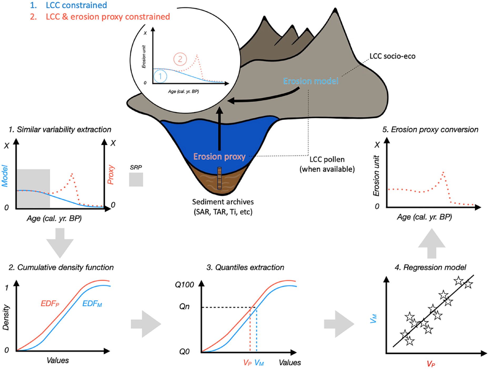
Methodological framework of the conversion method used in this study.

The combined use of erosion proxies and a soil erosion model will allow us to provide harmonized quantitative estimates of soil erosion within the study area. These new estimates result in a nearly twofold increase of the previous RUSLE-based estimations of soil erosion spanning the Holocene (i.e., Wang and Van Oost, 2019).

Materials and methods

Study sites

Six alpine lake watersheds have been used for this study (Petit Lac d’Annecy, Anterne, Benit, Moras, Paladru, and La Thuile) within the Northwestern Alps (Figure 2). These study lakes were chosen for the availability of terrigenous proxies in their respective lacustrine sediment sequences covering from the last 2000 years to the last 12,000 years (Table 1). All the study sites are of glacial origin and are distributed along a southwest to northeast altitudinal gradient with watershed maximum altitudes ranging from 420 meters above sea level (asl) for the Moras watershed to 2494 meters asl for the Anterne watershed (Table 2). The lake altitudes range from 304 meters asl for Lake Moras to 2063 meters asl for Lake Anterne. The average annual rainfall ranges from 960 mm.yr⁻¹ for Lake Moras to 1878 mm.yr⁻¹ for Lake Anterne (Table 2). Finally, three sites are known for the presence of gully erosion forms within their respective watershed (Anterne, Benit, and La Thuile), potentially indicating high erosion rates.

Figure 2.

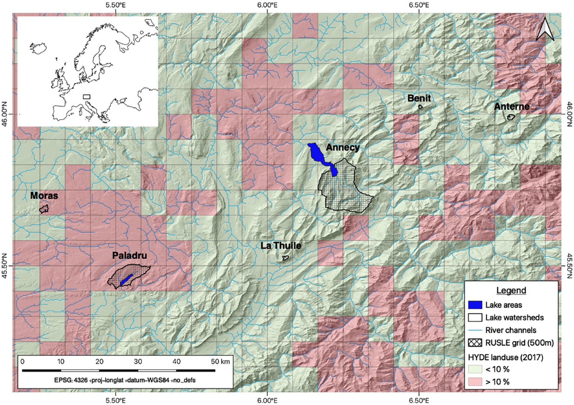
Location of the six study lakes and their watersheds in the Northwestern Alps.

Table 1.

Erosion proxies used in this study.

Site	Core	Erosion proxy	Time period (cal. yr. BP)	Source
Annecy	LA13	SAR (cm².yr⁻¹)	[0; 4350]	Jones et al., 2013
Anterne	ANT-07	SAR (cm.yr⁻¹)	[0; 9550]	Giguet-Covex et al., 2011
Benit	BEN14 & BEN16	TAR (mg.cm⁻².yr⁻¹)	[⁻50; 2110]	Bajard et al., 2018
Moras	MOR08-MC	TAR (mg.cm⁻².yr⁻¹)	[⁻50; 3950]	Doyen et al., 2013
Paladru	PAL09-MC	Ti (kcps)	[⁻50; 10025]	Doyen et al., 2016
Thuile	THU10	Erosion (t.km⁻².yr⁻¹)	[⁻64; 12010]	Bajard et al., 2017

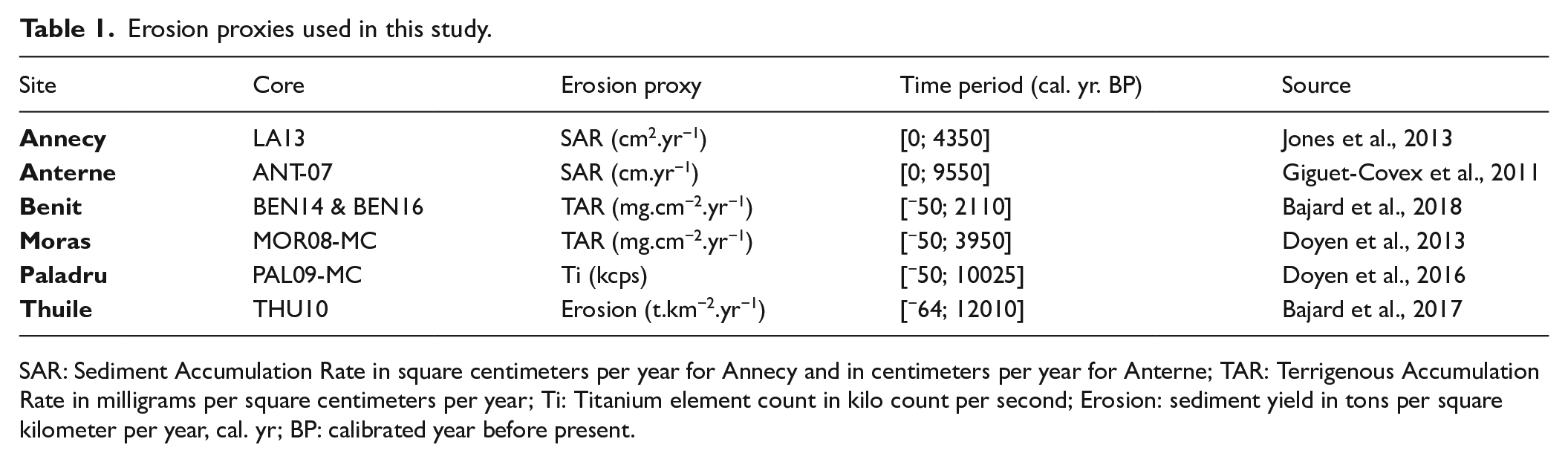
SAR: Sediment Accumulation Rate in square centimeters per year for Annecy and in centimeters per year for Anterne; TAR: Terrigenous Accumulation Rate in milligrams per square centimeters per year; Ti: Titanium element count in kilo count per second; Erosion: sediment yield in tons per square kilometer per year, cal. yr; BP: calibrated year before present.

Table 2.

Study sites features.

Site	Lake area (km⁻²)	Watershed area (km⁻²)	Lake alt. (m. asl)	Upstream watershed alt. (m. asl)	Annual rainfall (mm.yr⁻¹)	Gully erosion	Source
Annecy	26.5	170.4	460	2254	1646	No	Jones et al., 2013
Anterne	0.12	2.55	2063	2494	1878	Yes	Giguet-Covex et al., 2011
Benit	0.04	0.9	1450	2230	1110	Yes	Bajard et al., 2018
Moras	0.02	4	304	420	960	No	Doyen et al., 2013
Paladru	3.92	55	492	780	1160	No	Doyen et al., 2016
Thuile	0.06	1.6	874	1209	1600	Yes	Bajard et al., 2016

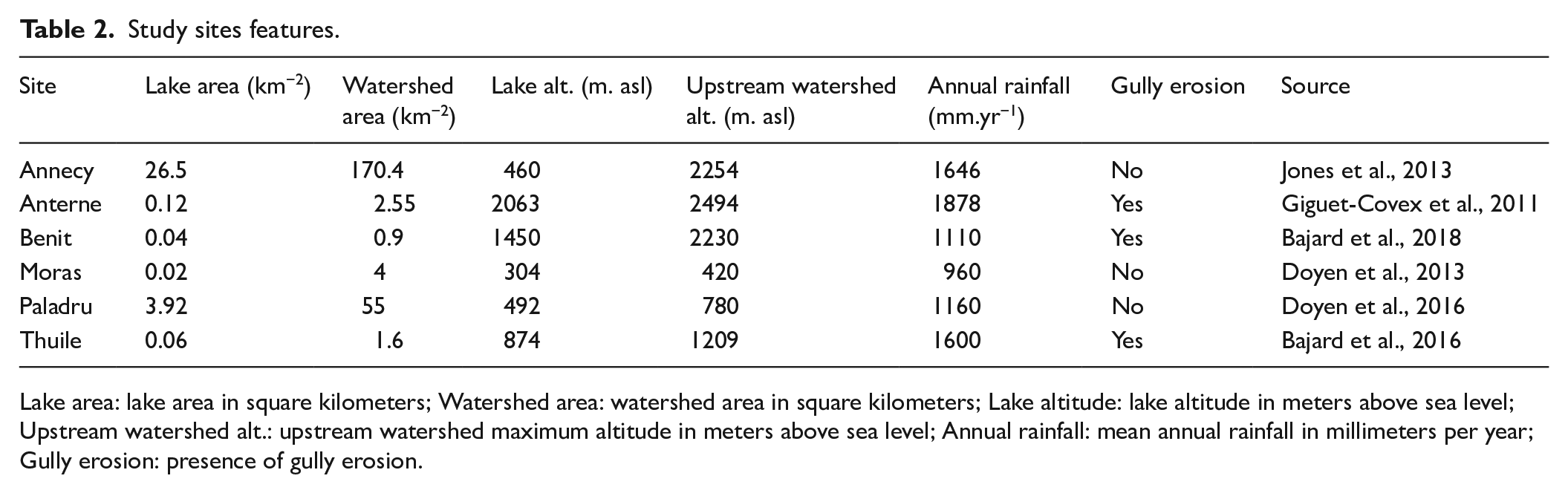
Lake area: lake area in square kilometers; Watershed area: watershed area in square kilometers; Lake altitude: lake altitude in meters above sea level; Upstream watershed alt.: upstream watershed maximum altitude in meters above sea level; Annual rainfall: mean annual rainfall in millimeters per year; Gully erosion: presence of gully erosion.

Available data

Proxies

Long-term monitoring of sediment loads in rivers around the world provides evidence for assessing recent changes in soil erosion, but such records rarely go back more than 50 years. Nonetheless, many opportunities exist to exploit the natural archives preserved within lake sediments, river banks, deltas, alluvial, and colluvial soils to extend contemporary records and provide evidence of changes in soil erosion over a range of time scales from decades to millennia. Among these archives, lake sediments can provide continuous records of erosion, also often called terrigenous inputs, at various scales corresponding to the size of the lake catchment.

Various proxies can be used to reconstruct the erosion dynamic (e.g., Giguet-Covex et al., 2023). The diversity of these proxies partly depends on the sedimentary fabric, itself being the result of physical, chemical, and biological features and processes (e.g., geological and climatic context, vegetation cover, topography). Another factor explaining the diversity of erosion proxies found in the literature is the access to instrumental measurements by the research teams. In this study, one terrigenous proxy has been selected per study site (Table 1). The choice was guided by the previous publications of the different study sites, most of which aimed to trace the erosion dynamic. Consequently, they proposed and used the most reliable proxy for assessing erosion dynamic in each system (Table 1). First, the continuous sediment accumulation rate (SAR; cm.yr^-1) is available for a period of 4350 years for Lake Annecy (LA13, Jones et al., 2013) and for a period of 9550 years for Lake Anterne (ANT-07, Giguet-Covex et al., 2011). SARs from lakes integrate three basic forms of sedimentary processes related to surface erosion, mass movement, and linear transport. Hence, SARs were computed for the lake-catchment where it was assumed that the lake productivity fluxes were relatively low or constant over time compared to allochtonous sources. Second, the terrigenous accumulation rate (TAR; mg.cm⁻².yr⁻¹) is available for a period of 2160 years for Lake Benit (BEN14 & BEN16, Bajard et al., 2018) and for a period of 4000 years for Lake Moras (MOR08-MC, Doyen et al., 2013). TAR has the great advantage of relating to allochtonous supplies only, and may be useful in reconstructing erosion from lake archives supplied by significant autochtonous fraction. The relative Ti content from XRF core scanner analyses (kcps) is available for a period of 10,075 years for Lake Paladru (PAL09-MC, Doyen et al., 2016). The erosion flux (t.km⁻².yr⁻¹) is available for a period of 12,075 years for Lake La Thuile (THU10, Bajard et al., 2017) and has been the only quantified data already available and directly exploitable as erosion unit within our study sites.

All proxies show a global increasing trend in soil erosion over the Holocene (Figure 3), that is, minimal values at the beginning of each record and slightly (e.g., Moras watershed) or significantly (e.g., Annecy watershed) increasing values up to the present time. Furthermore, some tipping points and/or abrupt peaks can be observed for all records. Based on this qualitative description, three main periods, not necessarily simultaneous, can be distinguished. The first and older period can be characterized by a low and relatively stable erosion rates with, in some cases, a slight increase of the signal toward the most recent period. The second period is characterized by an acceleration of soil erosion defining a tipping point in the signal described in some study sites as an “erosion crisis” (Arnaud et al., 2016; Bajard et al., 2017), that is, an ephemeral period of time of major erosion lasting from about a hundred to a thousand of years, and finally a period of slight but greater erosion increase corresponding to the post-“erosion crisis” period. These three Scientific References Periods (SRP) are called Pre-Crisis Period, Crisis Period, and Post-Crisis Period, respectively. The starting and ending dates of SRP defined based on the analyze of the signal structures, described above and discussed in the previous publications can be found in Table 3.

Figure 3.

Erosion trends in the six studied sites reconstructed from lake sediment records delimited for the three SRPs.

Table 3.

Scientific References Periods (SRP) definition and associated references.

Site	Source	SRP dates (cal. yr. BP)
Site	Source	Post-crisis	Crisis	Pre-crisis
Annecy	Higgitt et al., 1991; Jones et al., 2013	[0; 500]	[500; 2110]	[2110; 4350]
Anterne	Giguet-Covex et al., 2011	[0; 1300]	[1300; 5550]	[5550; 10165]
Benit	Bajard et al., 2018	[−50; 700]	[700; 1100]	[1100; 2110]
Moras	Doyen et al., 2013	[−50; 1600]	[1600; 2200]	[2200; 3950]
Paladru	Doyen et al., 2016	[−50; 1100]	[1100; 2200]	[2200; 9950]
Thuile	Bajard et al., 2017	[−64; 800]	[800; 2500]	[2500; 12010]

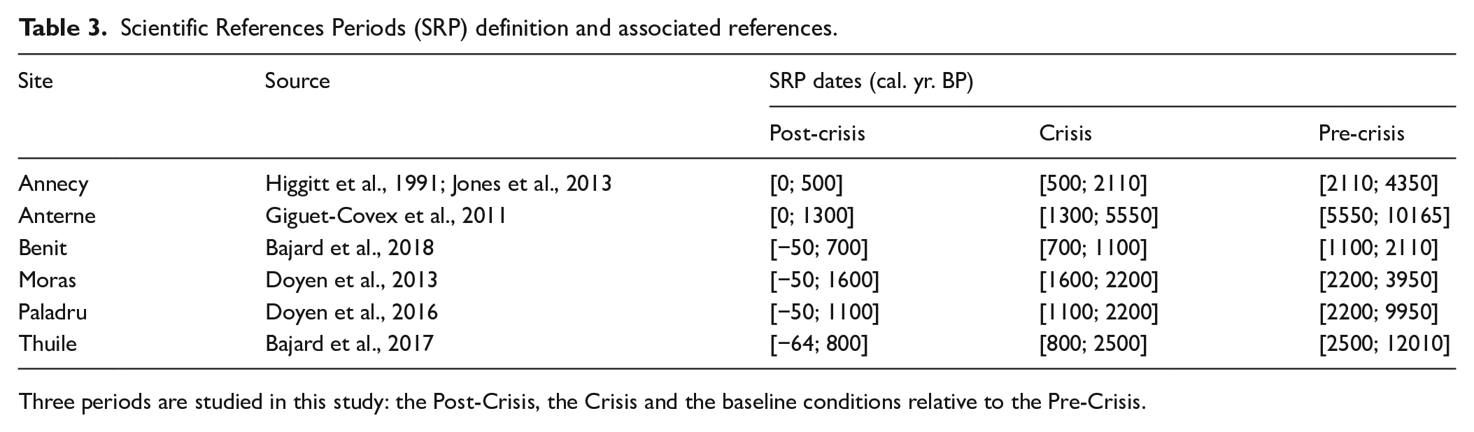
Three periods are studied in this study: the Post-Crisis, the Crisis and the baseline conditions relative to the Pre-Crisis.

At this point, despite the reliability of these proxies, conducting an intercomparison of erosion rates between the six sites is challenging due to the lack of a common quantitative information provided by these proxies, that is, there is no common unit. This limitation prompted us to perform erosion model simulations as a complementary approach, and the details of these simulations of erosion are presented below.

RUSLE-HYDE

The soil erosion production of each study site has been estimated with a RUSLE-based soil erosion reconstruction for the whole Holocene period. The well-known Revised Universal Soil Loss Equation (RUSLE, (Renard et al., 1997; Wischmeier and Smith, 1978)) is a semi-empirical model able to estimate the mean annual soil loss rate by sheet and rill erosions within a study area according to the following equation (1):

E = R * K * C * L S * P

(1)

where E (t.ha⁻¹.yr⁻¹) is the annual average soil loss, R (MJ.mm.ha⁻¹.h⁻¹.yr⁻¹) is the rainfall erosivity factor, K (t.ha.h.ha⁻¹.MJ⁻¹.mm⁻¹) is the soil erodibility factor, C (dimensionless) is the land cover-management factor, LS (dimensionless) is the slope length and slope steepness factor and P (dimensionless) is the support practices factor (farming direction, strip cropping, etc.) (Panagos et al., 2015b).

RUSLE has been yearly computed with the C factor varying each year according to the HYDE database landuse spatialization. While alternative land cover databases are available, the HYDE database provides a spatially distributed global reconstruction of anthropogenic land cover changes for the whole Holocene period (11,950 to −67 BP) for 75 dates with a spatial resolution of 5 arcmin (~85 km² at the equator) (Goldewijk et al., 2017). The HYDE database in this case was adapted to the regional scale of the study. The other RUSLE factors α_RKLSP (R, K, LS, & P) have been kept constant over time by using the respective RUSLE2015 raster grid of each factor (Panagos et al., 2015b). This means that the RUSLE erosion simulations variability is here only driven by the ALCC temporal variability in association with the other factors spatial variability (Supplementary Materials, Figure S5). In other terms, only the long-term impacts of ALCC on erosion have been simulated. Coupling effects with, for example, rainfall erosivity factor across time are not the purpose of this study. However, we also performed some analyses to test the potential significance of this factor (see section “Sensitivity analysis of RUSLE-HYDE”). Cropland, grazing, and natural forestland categories have been considered in the RUSLE-HYDE simulation (RUSLE-HYDE refers in what follows to this RUSLE model forced by the HYDE database). A respective C factor has been associated with each land use category according to the literature (Panagos et al., 2015a): 0.233 for cropland areas, 0.0903 for grazing land areas and 0.0001 for natural forestland areas (1):

E_{i} = α_{R K L S P} * ({L U}_{n a t i} * C_{n a t} + {L U}_{{g r a z}_{i}} * C_{g r a z} + {L U}_{{c r o p}_{i}} * C_{c r o p})

(2)

where E is the annual average soil erosion (t.km⁻².yr⁻¹), i is the ith simulated year, α_RKLSP is the RUSLE state parameter, LU_nat is the natural forestland fraction, LU_crop is the cropland fraction, LU_graz is the grazing land fraction, C_nat is the natural forestland C factor, C_crop is the cropland C factor, and C_graz is the grazing land C factor.

The range of the values simulated with RUSLE-HYDE are shown in Figure 4 for the six watersheds. It should be noted that the RUSLE-HYDE model did not simulate the erosion Crisis Period recorded by the proxies at the different sites. If the erosion model provides quantitative estimates but contradict the temporal trend shown by the proxies, it must be concluded that the proposed model and approach is not suitable for solving our problem. The idea then arises of whether it is possible to reconcile the presumably accurate temporal variability of erosion provided by the proxies (i.e., non-quantitative or semi-quantitative) with the quantitative estimates of the erosion model by developing an original approach based on statistics using the signals variability.

Figure 4.

Erosion trends simulated with erosion models for each individual Alpine study site, in tons per square kilometer per year.

RUSLE-PALEO: combine proxy-data with the RUSLE-HYDE model

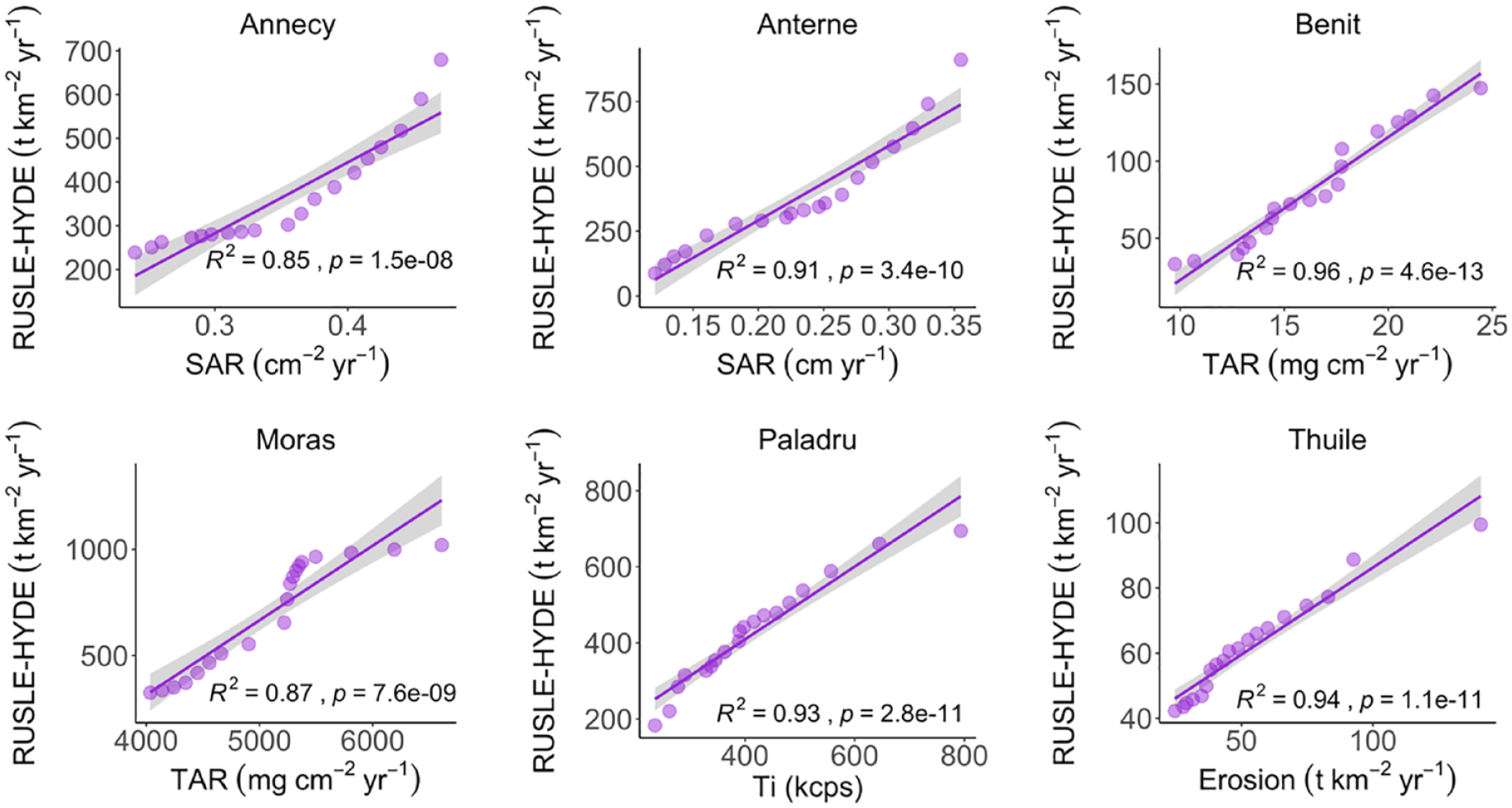
The approach proposed here to reconstruct the erosion dynamic quantitatively and in a way that is comparable across different locations and spatial scales consists in converting paleo-environmental data of erosion into erosion units by taking advantage of outputs from soil erosion models (RUSLE-HYDE model). In other words, the goal is to find the conversion function that allows to convert non quantitative or semi-quantitative proxies values into quantitative soil erosion values expressed with the same unit (t.km⁻².yr⁻¹) as with the RUSLE quantitative estimates. Directly comparing proxies and RUSLE-HYDE time series is not feasible. Indeed, as an example, linear regressions between RUSLE-HYDE and proxies show a weak correlation factor (cf. Table 4: R² raw data column; Supplementary Materials, Figure S6). This can be easily understood as the RUSLE-HYDE time series displays periods with variability comparable to that of the proxies (Post-Crisis Period), alongside periods with little variability, whereas the proxies exhibit high peak values (Crisis Period Figures 3 and 4).

Table 4.

Correlation metrics between erosion trends from model (RULSE-HYDE) and proxies (lake sediment records). Metrics are provided for raw data and after EDF conversion.

Site	Post-crisis SRP (cal. yr. BP)	R² (raw data)	R² EDF	Slope correlation	Scaling constant
Annecy	[0; 500]	0.66	0.85	1190.83	−45.44
Anterne	[0; 1300]	0.24	0.91	2062.28	−74.87
Benit	[−50; 700]	0.02	0.96	5.93	−11.54
Moras	[−50; 1600]	0.02	0.87	0.51	−1940.66
Paladru	[−50; 1100]	0.09	0.93	1.20	−86.89
La Thuile	[−64; 800]	0.10	0.94	1.00	1.17

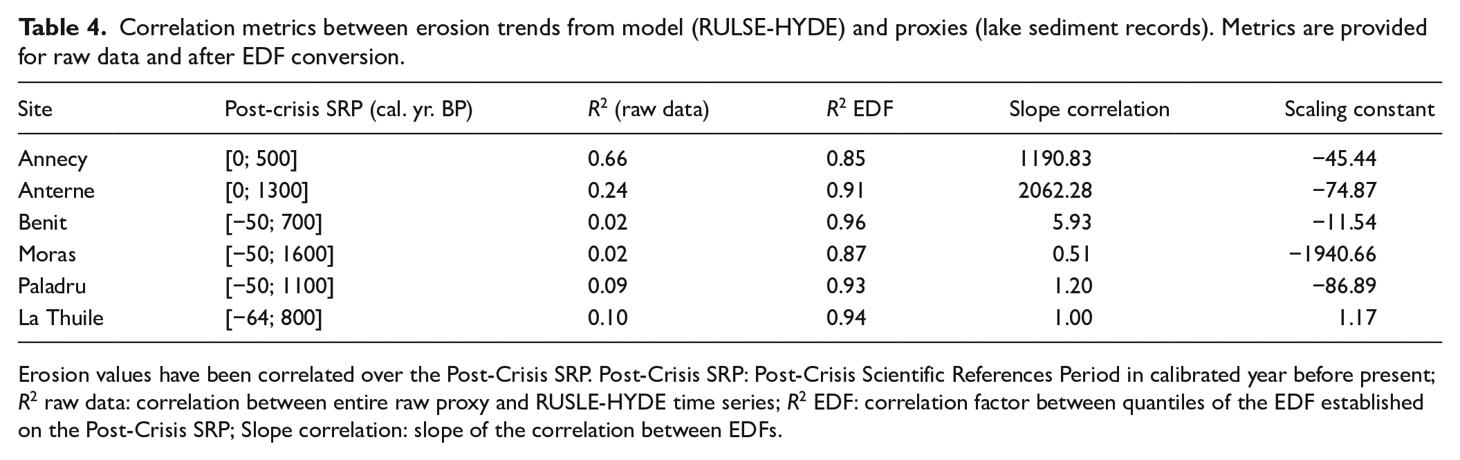
Erosion values have been correlated over the Post-Crisis SRP. Post-Crisis SRP: Post-Crisis Scientific References Period in calibrated year before present; R² raw data: correlation between entire raw proxy and RUSLE-HYDE time series; R² EDF: correlation factor between quantiles of the EDF established on the Post-Crisis SRP; Slope correlation: slope of the correlation between EDFs.

Our erosion signals incorporate both (1) temporal variability, representing periods of high/low signal variability, and (2) statistical variability, reflecting distributions of values with varying proportions of high/low values. Concerning temporal variability, it is noteworthy that numerous processes can take place along the watershed between the soil erosion production (simulated by the soil erosion model) and the cumulative sedimentation at the bottom of the studied lakes (measured by the proxy): deposition and remobilization on hillslope pathways (i.e., the sedimentary cascade that can be more or less significant in the different topographical contexts and can be expected to increase with the size of watersheds), lake hydraulic dynamics, etc. These processes are not considered by the RUSLE model. For these reasons, it cannot be assumed a priori that the proxy time series and the soil erosion model simulations are synchronous, as possibly large and varying time delays may occur between soil erosion and lake sediment accumulation (Hoffmann, 2015). This is the key assumption underlying the proposed approach to converting different erosion proxies into comparable erosion rates between sites. The conversion function has then to be established independently of the temporal variability of both proxies and RUSLE time series. But the statistical variability of both signals can still be considered as relevant and be used to build this conversion function.

A suitable mathematical tool to analyze the statistical variability of a signal independently of its temporal variability is the Empirical Distribution Function (EDF). An EDF is an estimate of the Cumulative Distribution Function (CDF) F, which can be defined for a real-valued variable X by the following equation (3):

F (x) = P (X \leq x)

(3)

where P is the probability that the variable X takes on a value less than or equal to x.

The EDF then takes the value 0 when x = x_min, and the value 1 when x = x_max, with x_min and x_max being the minimal and maximal values of a given sample, respectively. If the EDF of a given signal is a straight line, this means that the signal contains the same proportion of each range of its values (i.e., as much as low and high values). If the EDF is convex, this means that the signal contains a larger proportion of high values, and if the EDF is concave, this means that the signal contains more smaller values.

Once the EDFs of the proxy has been built, it can be confronted to the EDF of the associated RUSLE simulation. By selecting a given set of quantiles (Q), it is possible to establish a relation between the EDF of the RUSLE simulation and the EDF of the proxy signal by interpolating a function between the associated Q_RUSLE values and the Q_Proxy values for the chosen set of quantiles (4):

Q_{R U S L E} = f (Q_{P r o x y})

(4)

In this study, a set of quantiles from 10% to 100% by steps of 5% have been chosen to sample the different EDFs. Also, without any proven reason to use more complex approach, a simple linear interpolation has been established between the quantile values of the RUSLE’s EDF and the quantile values of each proxy’s EDF (5):

Q_{R U S L E} = a . Q_{P r o x y} + b

(5)

where a is the slope correlation, b is the intercept value.

Reaching this point, it is now possible to convert non quantitative proxies’ values into quantitative values with the RUSLE simulation.

Altogether, the step by step method summarized in Figure 1 consists in:

Extract the data of both proxy and RUSLE data on the time period with the most similar statistical variability between the two signals, the Post-Crisis Period SRP in our case.

Build the EDFs of both proxy and RUSLE data subseries.

Associate each value of both proxy and RUSLE data to the chosen set of quantiles (from 10% to 100% by steps of 5% in our case) from its respective EDF.

Establish a regression model between the paired values of the proxy’s EDF and the RUSLE’s EDF, a linear relationship in our case (Figure 5).

Convert the proxy into a quantitative RUSLE value with the regression model.

The question remains of choosing the relevant time period to set up the EDFs correlation. As mentioned above, the Crisis Period is obviously not suitable for comparison between proxies’ time series and RUSLE simulations as the RUSLE simulations deeply fails to simulate this peak variability. The Crisis Period has then not been considered to establish proxies’ conversion functions. The Pre-Crisis Period shows little variabilities for proxies and nearly constant values of the RUSLE simulation (Figure 4): it makes little sense to correlate a signal with a quasi-constant or event constant signal. This period is then not suitable for the EDFs correlation, but it is worth noting that this period is in a way still taken into account as it represents the minimal values for proxies time series and RUSLE simulations, minimal values which are used in the method described before. It appears then that the period with the most similarity between the proxies and RUSLE-HYDE statistical variabilities is the Post-Crisis Period, that is, the period from the present to the end of the Crisis Period.

Due to the interpolation, it is not certain that the converted proxy value will be greater or equal to zero at this step, as it should be. To ensure that the converted proxies have all values greater or equal to zero instead of using raw values of proxies and RUSLE simulations, the method has been applied on the values of proxies minus their minimum value on the all Holocene period and on the values of RUSLE minus their minimum value on the all Holocene, which is corresponding in all cases to the minimum value of the Pre-Crisis Period. Furthermore, the linear interpolations have been performed forcing the intercept term to be equal to zero and the final relationship between the Q_RUSLE values and the Q_Proxy values has been corrected from their respective minima with a scaling constant c (Table 4).

The method suggested here has then been applied for the six watersheds on the Post-Crisis Period. In what follows, the converted erosion proxies using RUSLE in the study watersheds are called RUSLE-PALEO data (Figure 4).

Estimation of uncertainties

Erosion proxies conversion

The confidence interval of each EDF has been estimated with the Dvoretzky-Kiefer-Wolfowitz (DKW) inequality (Dvoretzky et al., 1956) (6):

P (L (x) \leq F (x) \leq U (x) f o r a l l x \geq 1 - α

L (x) = \min {F (x) + ε, 1}

U (x) = m a x {F (x) - ε, 0}

ε = \sqrt{\frac{1}{2 n} l n \frac{2}{α}}

(6)

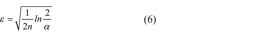
where ε is the margin of error, n is the number of data points and α is the confidence level.

The DKW inequality has been applied on the EDF distribution of each study site (Supplementary Materials, Figure S3) to approximate the uncertainties of RUSLE-PALEO.

Sensitivity analysis of RUSLE-HYDE

The inherent limitations of the RUSLE model to represent some key processes of erosion like soil incision (e.g., gully erosion) and the limited forcing data available (mainly for rainfall and soil erodibility) do not allow us to explore the specific controlling factors of erosion over long-term trends, but rather to investigate whether the simulated erosion values are included within realistic orders of magnitude. Despite these limitations, it is probably reasonable to assume that there does exist a “natural variability” of the forcings factors throughout the Holocene. Additionally, an “anthropogenic variability” could have been triggered by human activities over short-term periods, in particular during Crisis Periods. The effects of these two variabilities on erosion can be tested using a sensitivity analysis, targeting a range of realistic values of the forcing factors of the erosion model.

The landuse intensity, the rainfall erosivity, and the soil erodibility have been considered as the most relevant forcing factors to explain long-term erosion dynamics in the Northwestern Alps according to the hypothesis raised by Bajard et al. (2016, 2017), Giguet-Covex et al. (2011, 2014, 2023) in this specific region. Indeed, according to the non-arboreal pollen data in most of our study sites (Supplementary Materials, Figure S1), there were low landscape opening intensities during the Pre-Crisis Period, then a clear increase in landscape opening appeared during the Crisis Period, suggesting a strong variation in land cover change, and finally the Post-Crisis Period has experienced a higher intensity of landscape opening than in the Pre-Crisis Period. At the alpine scale, annual rainfall appears to have remained fairly stable over the last 8000 years according to Arthur et al. (2023), but the uncertainty of the rainfall estimations is about 50%. In several study sites, the organic horizons of the soils formed during the Early to Mid-Holocene period have given way to deeper and more erodible horizons over the most recent periods (marls in La Thuile watershed, flysch rocks in the Bénit watershed and black shales, calcshales and shales in Anterne).

The sensitivity analysis of RUSLE-HYDE has been conducted with six scenarios of landuse intensity (C factor), rainfall erosivity (R factor), and soil erodibility (K factor) (Supplementary Materials, Table S1). These scenarios consider the influence of both natural and anthropogenic potential variabilities on soil erosion according to realistic variations in the identified forcing factors over the whole Holocene period, and more specifically during the Crisis Period of each study site. The natural variability has been simulated with variations of ±20%, and the anthropogenic variability has been simulated with variations greater than ±20%.

Results and interpretations

Method corroboration

The relationships between proxies’ quantiles and RUSLE-HYDE quantiles are relatively linear in the chosen period and led to acceptable correlation coefficients compared to the raw correlation coefficients between the RUSLE-HYDE and the proxies from the full periods, except for the Annecy and Anterne watersheds (Figure 4 and Table 4). Moreover, the slope correlation factor from the linear regression is equal to 1 on the La Thuile watershed (Table 4). This is reassuring, as the La Thuile proxy is already expressed as a soil erosion unit (the only one among the six watersheds). It is worth noting that this small watershed with steady slopes, a short hillslope length, and a simple lake watershed shape is expected to have a close relationship between soil erosion production and sediment accumulation in its lake. It was then hoped that the conversion relationship would give a slope factor close to 1, as it is the case. This is then a good corroboration test for the method suggested in this paper.

RUSLE-HYDE underestimation

The Relative Difference (RD) between RUSLE-PALEO and RUSLE-HYDE has been estimated using the following equation (7):

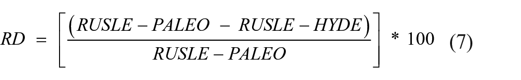
R D = [\frac{(R U S L E - P A L E O - R U S L E - H Y D E)}{R U S L E - P A L E O}] * 100

(7)

where RD is expressed in percentage RUSLE-HYDE and RUSLE-PALEO are both expressed in t.km⁻².yr⁻¹.

The RD for our six sites shows an underestimation of RUSLE-PALEO by RUSLE-HYDE ranging from 3% for Annecy to a maximum of 60% for Anterne, with an overall underestimation of 51% for all the sites (Table 5). This means that modeling soil erosion with HYDE is omitting close to the half of soil erosion exports during the Holocene, at least within our study sites. This underestimation is mainly due to the failure of RUSLE-HYDE to reproduce the Crisis Periods.

Table 5.

Estimates of soil denudation and erosion rates from RUSLE-PALEO.

Site	Denudation (cm)		Erosion (t.km−².yr−¹)					Proportions (%)
Site	Total DD	Crisis DD	Mean full period	Mean post-crisis	Mean crisis	Mean pre-crisis	Confidence interval	Total RD	Part crisis
Annecy	33.84 ± 16.92	15.43 ± 6.17	155.36	364.60	132.87	23.10	±49.82	3.87	45.59
Anterne	106.34 ± 16.38	68.02 ± 7.31	195.11	390.52	264.09	11.80	±22.35	60.45	63.97
Benit	9.56 ± 7.43	4.02 ± 1.40	88.27	83.65	150.56	19.65	±45.55	38.01	42.09
Moras	268.91 ± 163.29	140.90 ± 26.19	1564.53	640.58	3107.09	118.45	±568.48	53.91	52.40
Paladru	95.47 ± 36.83	33.15 ± 4.01	223.38	390.03	593.52	52.63	±47.49	54.08	34.73
La Thuile	10.81 ± 1.73	6.77 ± 0.24	69.62	49.65	130.35	1.67	±1.87	23.81	62.61
Sites	524.91 ± 242.58	268.29 ± 45.32	382.71	319.84	729.75	37.88	±122.59	51.13	51.11

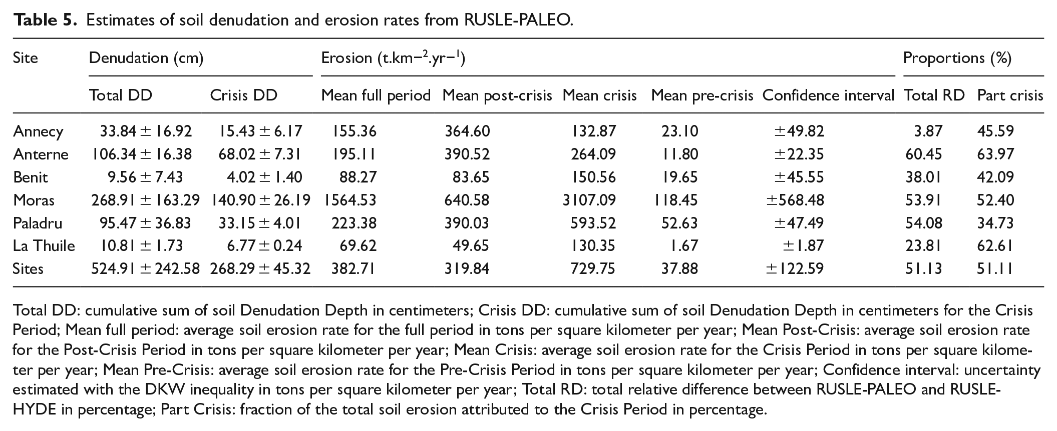
Total DD: cumulative sum of soil Denudation Depth in centimeters; Crisis DD: cumulative sum of soil Denudation Depth in centimeters for the Crisis Period; Mean full period: average soil erosion rate for the full period in tons per square kilometer per year; Mean Post-Crisis: average soil erosion rate for the Post-Crisis Period in tons per square kilometer per year; Mean Crisis: average soil erosion rate for the Crisis Period in tons per square kilometer per year; Mean Pre-Crisis: average soil erosion rate for the Pre-Crisis Period in tons per square kilometer per year; Confidence interval: uncertainty estimated with the DKW inequality in tons per square kilometer per year; Total RD: total relative difference between RUSLE-PALEO and RUSLE-HYDE in percentage; Part Crisis: fraction of the total soil erosion attributed to the Crisis Period in percentage.

Soil erosion quantification and study sites inter-comparison

The aim of our approach based on statistics is to convert diverse erosion paleo-proxies of erosion into a signal with a unique, and thus comparable, unit. Such approach may contribute to intercompare watersheds behaviors using proxies that are not easily quantitively comparable at first (Figure 4).

The average RUSLE-PALEO erosion rate for the six watersheds is approximately 383 [70; 1565] t.km⁻².yr⁻¹ for the full period (Table 5), revealing notable differences among the study sites with for instance estimated erosion values nearly 30 times greater for the Moras watershed than for the Benit watershed. Erosion estimates for the Post-Crisis Period (320 [50; 641] t.km⁻².yr⁻¹) align with estimations from other studies conducted in the Alps for the last century, ranging from 385, 450, to 527 t.km⁻².yr⁻¹ (Hinderer et al., 2013; Panagos et al., 2015b; Vanmaercke et al., 2011) and of 343 t.km⁻².yr⁻¹ for Europe (Fendrich et al., 2022). Though, the overall variability of erosion rates of the six study sites during the Post-Crisis Period is comparable with the variability in the Alps, but is really much higher than the variability in Europe (Figure 6). The range of variation recorded in watersheds ranging from the mountainous to the nival belts (La Thuile, Bénit, and Anterne) is also close to the estimations provided for two periods, in 1950s and in 2016, for the municipality of Montaimont, which cover the same vegetation belts and integrate similar landuse (2900 and 1600 t.km⁻².yr⁻¹, respectively) (Elleaume et al., 2022). The erosion estimates are much higher for the Crisis Period (730 [130; 3,107] t.km⁻².yr⁻¹) for most of the study sites, especially in Moras, Paladru, Benit, and La Thuile, compared to the Post-Crisis Period (320 [50; 641] t.km⁻².yr⁻¹) and the Pre-Crisis Period (38 [2; 118] t.km⁻².yr⁻¹) (Table 5 and Figure 6), This is underlying the major impact of transient erosion crisis on erosion rates during the Holocene in the Northwestern Alps with an average 20-fold increase in erosion rates from the Pre-Crisis conditions to the Crisis Period. Of course, these average values are given as rough estimates as they were not calculated on the same time periods (Figures 5 and 6), but one may still consider them as indicators of (1) the intensity of erosion within each study watershed, and thus of their erosion sensitivity and (2) of the spatial and temporal variability of this erosion intensity within the study area, especially considering the different erosion regimes during the Pre-Crisis Periods, the Crisis phases, and the Post-Crisis Periods.

Figure 5.

Correlation metrics (R² and p-value) between model (RULSE-HYDE) and proxies (lake sediment records) data after the EDF conversion.

Figure 6.

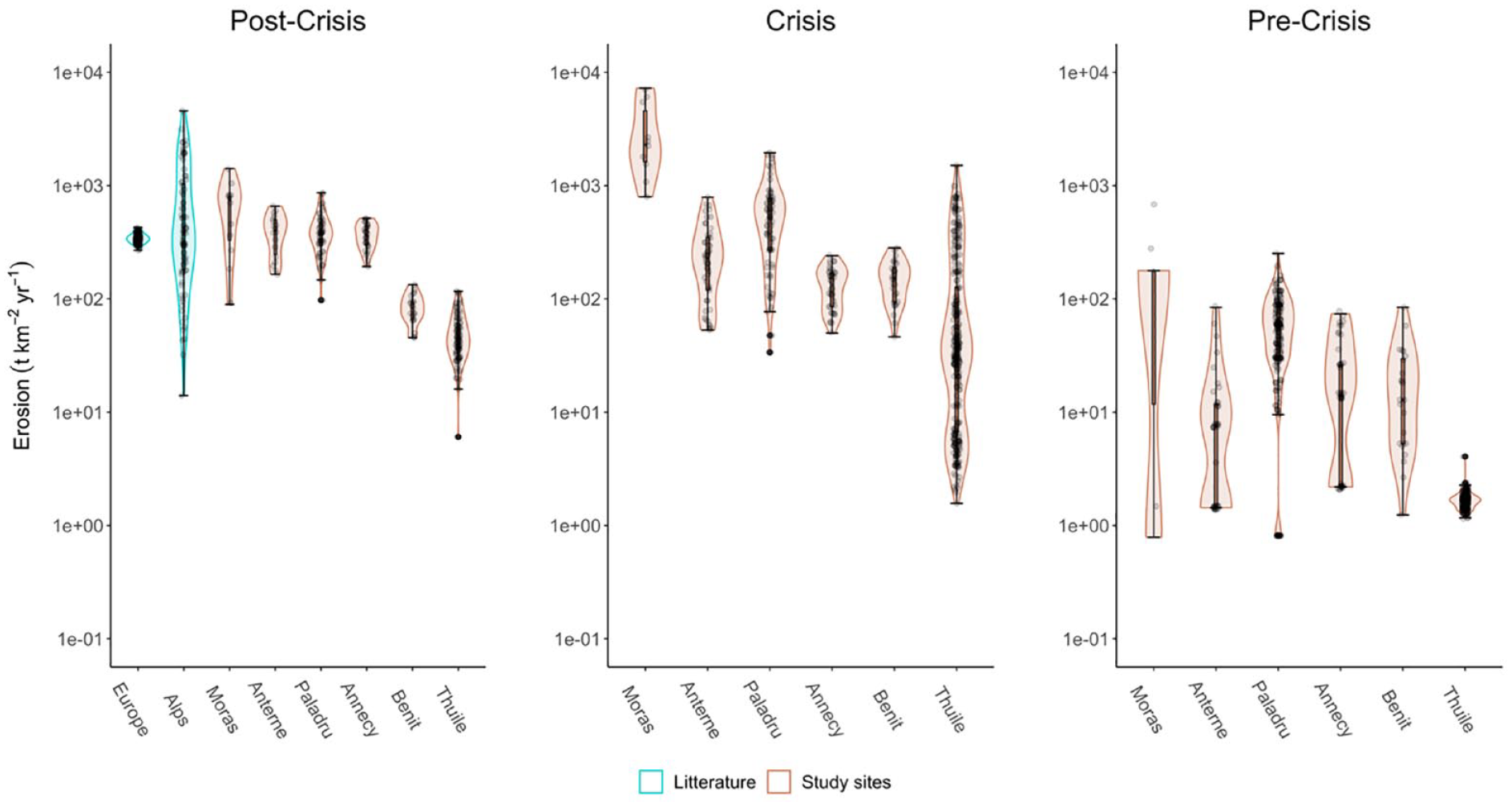
Soil erosion estimates for the Post-Crisis (left panel), for the Crisis (middle panel) and for the Pre-Crisis (right panel) Periods in the six study sites.

Regarding the total soil denudation calculated based on Bajard et al., 2017; Hinderer et al., 2013 with a mean bulk density of the soil of 1.3 g.cm⁻³ (Bajard et al., 2017), the Crisis Period represents approximately 51% of the total sediment export during the Holocene in our study sites (268 ± 45 cm for the Crisis Period versus 525 ± 243 cm for the whole Holocene period; Figure 7, Table 5). This clearly shows that significant amounts of soil have been lost in the study watersheds during this period.

Figure 7.

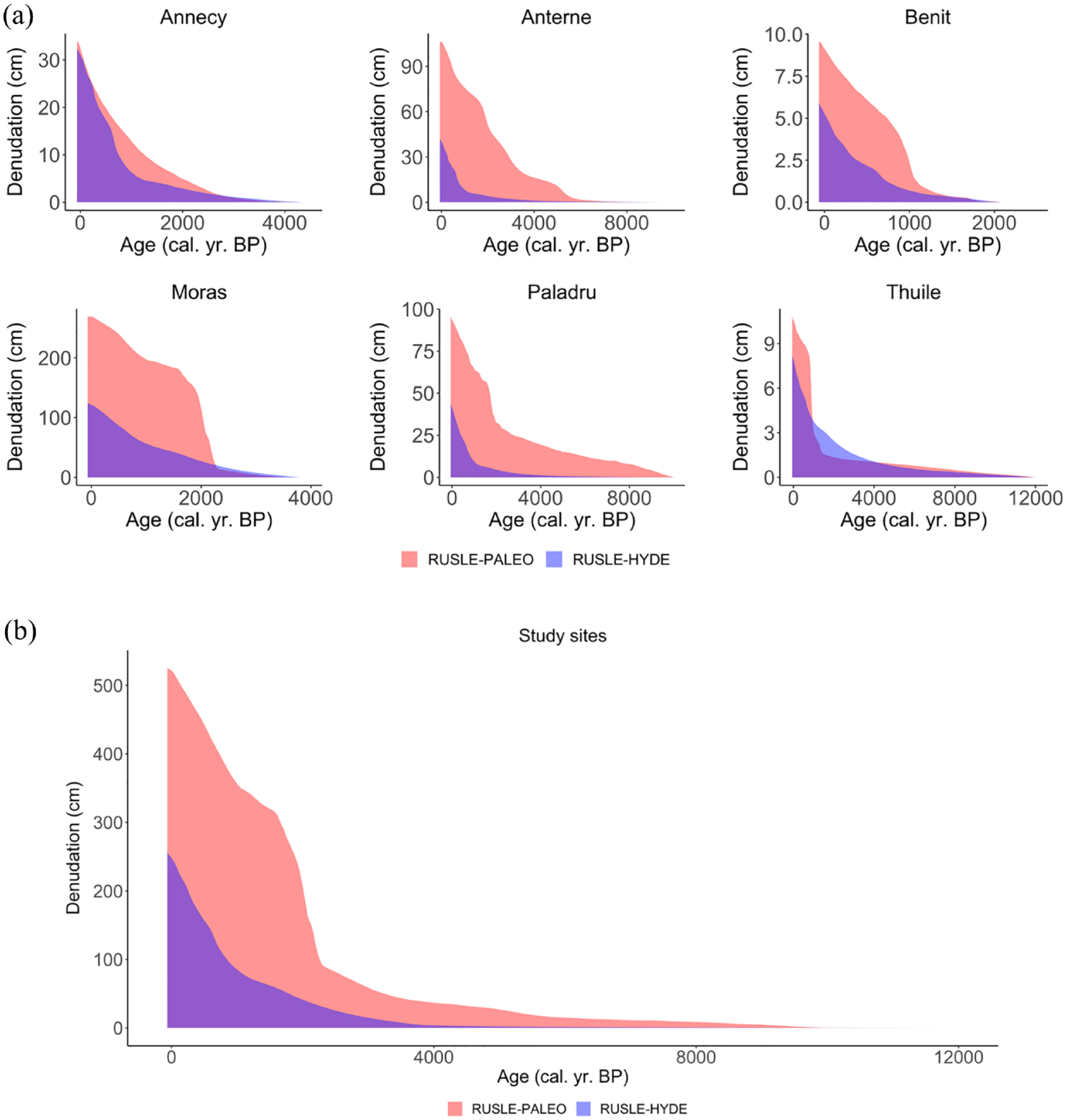
Cumulative soil denudation depth (cm) simulated by RUSLE-PALEO (red) and RUSLE-HYDE (blue). Panel (a) presents the results per study site, while panel (b) displays the cumulative sum for all the study sites.

Sensitivity analysis

The study sites do not respond equally to the chosen scenarios (Supplementary Materials, Table S1; Figure S4). For example, the scenario which best represents the erosion rates estimated for the Annecy watershed corresponds to the RUSLE-HYDE S0 scenario, i.e. by varying the C factor by + or - 20%. For the Moras and Paladru watersheds, the erosion rates simulated for the Crisis Period are reached close to the RUSLE-HYDE S4 scenario, that is, by varying the C factor by +500 or −50% and the R and K factor by + or –50%. For the La Thuile watershed these values are reached close to the RUSLE-HYDE S6 scenario that is, by varying the C factor by +2000 or −50% and the R and K factor by + or −50%. What these scenarios have in common is that the erosion rates of the Crisis Periods were achieved by changing substantially the C factor, in other word the land cover-management factor.

Discussions and perspectives

Method limitations and opportunities

Some limitations and cautions can be raised. The choice of the erosion model may itself be questioned. The parsimonious RUSLE modeling approach is largely used by the soil community (e.g., Borrelli et al., 2020; Efthimiou, 2014; Naipal et al., 2015; Rozos et al., 2013). Nevertheless, the RUSLE model has limitations. For example, this model is fitted to compute average annual sheet and rill erosion and is not appropriate to compute gully erosion or extreme seasonal erosion events. Using RUSLE to reconstruct Holocene erosion is then recommended for watersheds that have few or no occurrences of gully erosion. Alternatively, one should consider employing our approach by using a more complex model capable of reproducing gully erosion, such as the Erosion Potential Model (EPM) (Gavrilović, 1962). In our study, only three lake-watersheds recorded gully erosion, with limited extension in terms of area, over the six study sites. Consequently, erosion fluxes related to gully erosion should have been only minimally underestimated. This statement is also supported by the good linear correlation with a slope close to 1 between the proxy-based estimation of the erosion rates (Bajard et al., 2017) and the output of the RUSLE-PALEO approach at La Thuile, that is, one gully-affected site (Figure 4). In our study, it is then not assumed that the use of RUSLE significantly affected our overall methodological development. Still, the ease of use of the RUSLE model provides an interesting tool to estimate long-term erosion dynamics at various spatio-temporal scales once these limitations have been taken into account. In a broader perspective, erosion models can also be useful to estimate processes and forcings involved in erosion dynamics and/or testing hypothesis.

The erosion model has been forced in this study by the HYDE database. In the same way, one could question this choice. HYDE provides land use change reconstructions based on population density fluctuations over time. Other datasets exist to reconstruct past land cover that could be considered as viable alternatives to HYDE: pollen or sedaDNA datasets (e.g., Messager et al., 2022; Noël et al., 2001; Roberts et al., 2018) and vegetation dynamic models (e.g., Anderson et al., 2006; REVEALS, Githumbi et al., 2022; Marquer et al., 2020; LOVE, Sugita, 2007). Each of these methods, along with HYDE, have their own limitations, especially when applied over long time periods. Indeed, for instance, raw pollen or plant sedaDNA data are not producing a quantification of the land cover, but only relative changes. Furthermore, pollen provides local and regional signals and the exact source areas of pollen from the different species are not well known. On the contrary, sedaDNA origin is limited to the catchment area, but taphonomic issues of changes in the sources contributing to the signal may bias the reconstructions of the land cover at the catchment scale (Giguet-Covex et al., 2019, 2023; Morlock et al., 2023). However, as sedaDNA is expected to be transferred mainly by erosion processes, we expect this tool to be highly relevant for tracking land cover evolution specifically in areas affected by erosion (Giguet-Covex et al., 2023; Morlock et al., 2023). Vegetation modeling from pollen records provide quantitative data but also has limitations linked to model assumptions and to the spatial resolution of the model that don’t really fit with the catchment scale. Because of these limitations, there is a risk that these methods do not entirely reproduce the true variations in past land cover changes, potentially leading to discrepancies and asynchrony between the RUSLE model based on these reconstructions and the erosion signal recorded in the sediment core. The development of our method allows us to overcome these limitations by focusing on the range of values rather than their exact synchronicity. Therefore, we recommend the use of land cover reconstructions that, at the very least, allow the erosion signal to be accurately reproduced during periods covering a wide range of values, such as those recorded during the Post-Crisis Periods in our study areas, in order to be able to apply our proposed conversion method (see method section).

Our method is model-dependent because it relies on the calibration of the simulated erosion rates, but is also erosion proxy-dependent because it relies on the temporal variability of the proxy used in the conversion. In our case, we have considered the most relevant terrigenous proxy possible and available per study site. They differ from one site to another, and some proxies are best fitted to represent the incoming sediment yield from the watershed. Consequently, the quality of the outputs between our study sites is variable, which explains why we remained very general in the section “study site intercomparison.” One may consider that the “ideal” proxy would integrate only the terrigenous supplies from the watershed and its conversion in flux in g.cm⁻².yr⁻¹, by using also the sedimentation rate and the dry sediment density (i.e., TAR in Benit and Moras, Arnaud, 2014; Bajard et al., 2018; Doyen et al., 2013). However, this proxy does not consider the organic contribution to the terrigenous input, but only the minerogenic ones, and may thus underestimate the erosion estimates. Furthermore, we have to keep in mind that such quantifications, especially the amplitude of changes, can be significantly affected by the uncertainties in the age-depth model. The more constrained the age-depth model, the better the quality of the erosion signal. Another proxy that may be considered as “a very good proxy,” is the erosion rate, that is, the variable we also want to model for inter-site comparisons. The estimation of this erosion rate also requires the calculation of the TAR, but to extrapolate it then at the basin scale to estimate the entire catchment export (i.e., multiplying the TAR by the corresponding deposit surface for each sediment depth, for instance by assimilating the shape of the sedimentary fill to an ellipsoid) and to normalize it by the whole catchment surface (i.e., erosion rate in La Thuile; Bajard et al., 2017). In highly detrital systems with no significant variations of the dry sediment density as in Anterne (see Supplementary Materials, Figure S7 a), the sedimentation rate can be considered as a robust enough proxy. Finally, in lakes, where the autochtonous fraction can be significant and where no estimations of the dry density and/or of the minerogenic element contribution (%) are available, XRF core scanner measurements of a purely terrigenous element poorly affected by weathering processes may be used as alternative to the TAR and sedimentation rates (e.g., Ti at Lake Paladru). In conclusion, we recommend the use of the most realistic simulated erosion rates, at least for the period used for the correlation, and of the best erosion proxy to minimize uncertainties in the final erosion estimates. Additionally, this methodology would certainly benefit from further applications in other lake-watersheds and with several erosion proxies available by study site to assess the variability related with the choice of the proxy and the robustness of the method. As an example, the method has been tested with another proxy of erosion for Lake Anterne, the TAR. The quantification of erosion with the latter proxy is close to the one with the SAR with a Root Mean Square Error (RMSE) metric of 8.23 t.km⁻².yr⁻¹ between RUSLE-PALEO-SAR and RUSLE-PALEO-TAR for the full period (see Supplementary Materials, Figure S7 b).

Erosion crises implications on soil resources and drivers

Our study suggests that Crisis Periods appear to be highly conducive to erosion exports with likely high impacts on the watershed’s soils. Indeed, such Crisis Periods represent up to 64% of the total Holocene sediment exports in the study sites on a relatively short period of time, spanning approximately 1000 (±500) years and mainly occurring during the Late-Holocene (from 3000 to 1000 cal. yr. BP). As discussed in Bajard et al., 2017, a non-return threshold of soil erosion in the Thuile watershed was exceeded during the crisis, with erosion exports higher than 1000 t.km⁻².yr⁻¹. A nonreturn threshold of soil erosion has also been described in the Anterne watershed corresponding to erosion rates above 300 t.km⁻².yr⁻¹ from 3400 cal. yr. BP (Giguet-Covex et al., 2011). At La Thuile, it has been shown that above the non-return threshold reached during the crisis, soil formation cannot offset erosion exports, resulting in massive soil loss by exceedance of the tolerable erosion limit of the soil (Bajard et al., 2017). Our estimates of soil loss thickness during the crises represent a total soil denudation of 268.29 ± 45.32 within the study sites. However, as RUSLE is only considering the erosion of the fine earth fraction, our estimation of soil loss underestimates by 50% the previous estimations for Lake La Thuile (respectively 22 and 10 cm in Bajard et al., 2017) where they considered a soil skeleton composed of 50% coarse elements and plant macroremains. Following the assumption that soil is not fully composed of fine particles by increasing our estimates by 50% (Egli et al., 2001, 2014), our estimations would align with previous quantifications of soil denudation for Lake La Thuile with a Holocene total soil loss of 22 ± 3.46 centimeters and a crises total soil loss of 13.54 ± 0.48 cm.

The drivers of these Crisis Periods are still not fully understood, and it would be relevant to better understand their causes. A concomitant land openness acceleration with the Crisis Periods has been detected in the empirical land openness signal of most of our study sites (Supplementary Materials, Figure S1 and Figure S2). Moreover, the sensitivity analysis of RUSLE-HYDE shows that small variations in ALCC do not appear to explain all the erosion observed in our study sites (Supplementary Materials, Figure S4). If a variation of ±20% in the C, R and K factors seems to be sufficient to explain the natural variability of erosion within the Post-Crisis and Pre-Crisis Periods, the only scenarios that permitted to reach the highest erosion rates observed during the Crisis Period have been obtained with significant variations in the C factor. This is evidencing the important sensitivity of erosion to ALCC even during transient time periods. For instance, the maximum C factor value for the Crisis Period in the La Thuile watershed is 0.149 between RUSLE-HYDE S5 and S6 scenarios. This value can be related to high intensity pastoral and mid intensity agricultural activities C factor values according to Panagos et al., 2015a, which is consistent with the pollen diagram and sedaDNA data of this site (Bajard et al., 2016). The Crisis Period is also better simulated for an increase of 50% of the K factor, that is, of the soil erodibility factor, which corresponds to a value of 0.043. Such a K factor value is in the range soils with a medium fine texture (0.029–0.049; Panagos et al., 2014) and not in the range of organic soils (0.019–0.033; Panagos et al., 2014), which may suggest a high contribution of deeper horizons compared to organic soil surface horizons. The concordance of the RUSLE-PALEO estimates with these scenarios seems to agree with the hypothesis that transient erosion crises have been mainly caused by considerable changes in land cover changes by landscape opening. Indeed, landscape opening could have triggered negative feedbacks on soil by increasing its susceptibility to rainfall erosivity and by causing incision in top soil horizons. Hence, further work is needed to consolidate these scenarios to trace back the most realistic causes of erosion crises in the Northwestern Alps.

Conclusion

The method presented here shows that it may be possible to convert non-quantitative or semi-quantitative proxies to quantitative soil erosion estimates by combining well dated paleo-records and a soil erosion model. This allowed, at least in the watersheds studied here, to show the transient erosion crises have significantly impacted the erosion rates during the Holocene. Not considering these Crisis Periods leads to a significant underestimation of the anthropogenic perturbation of the erosion cycle. Global databases of ALCC such as HYDE are of great interest to force erosion models. However, their scale may not be suitable, at least until now, to describe local-scale transient erosion dynamics despite their relatively great impact along the land-ocean continuum. This could speak in favor of the consistent integration of paleo-data (i.e., erosion, pollens) into soil erosion modeling approaches.

Supplemental Material

sj-docx-1-hol-10.1177_09596836241254485 – Supplemental material for Half of the soil erosion in the Alps during the Holocene is explained by transient erosion crises as a consequence of rapid human land clearing

Supplemental material, sj-docx-1-hol-10.1177_09596836241254485 for Half of the soil erosion in the Alps during the Holocene is explained by transient erosion crises as a consequence of rapid human land clearing by Théo Mazure, Georges-Marie Saulnier, Charline Giguet-Covex, Pierre Sabatier, Manon Bajard, Vincent Chanudet, Fabien Arnaud and Jean-Philippe Jenny in The Holocene

Footnotes

Acknowledgements

We also thank the work of the anonymous referees who have participated to the improvement of the paper.

Author contributions

Théo Mazure: Conceptualization; Data curation; Formal analysis; Investigation; Methodology; Writing – original draft; Writing – review & editing

Georges-Marie Saulnier: Conceptualization; Data curation; Formal analysis; Investigation; Methodology; Writing – original draft; Writing – review & editing

Charline Giguet-covex: Conceptualization; Writing – review & editing

Pierre Sabatier: Writing – original draft; Writing – review & editing

Manon Bajard: Writing – original draft; Writing – review & editing

Vincent Chanudet: Writing – original draft; Writing – review & editing

Fabien Arnaud: Writing – review & editing

Jean-Philippe Jenny: Conceptualization; Funding acquisition; Methodology; Supervision; Writing – original draft; Writing – review & editing

Code and results availability

The code and the results reported in this paper can be accessed by asking the corresponding author.

Funding

The author(s) disclosed receipt of the following financial support for the research, authorship, and/or publication of this article: We acknowledge the financial support of this research by the ANR-20-CE01-0011 C-ARCHIVES.

ORCID iDs

Théo Mazure

Charline Giguet-Covex

Fabien Arnaud

Supplemental material

Supplemental material for this article is available online.

References

Anderson

Bugmann

Dearing

, et al. (2006) Linking palaeoenvironmental data and models to understand the past and to predict the future. Trends in Ecology & Evolution 21(12): 696–704.

Arnaud

(2014) Habilitation thesis. Savoie University. https://www.researchgate.net/publication/271729609_HDR_Fabien_Arnaud_-_Livre_1_-_2014?channel=doi&linkId=54d096ca0cf20323c217d437&showFulltext=true

Arnaud

Poulenard

Giguet-Covex

, et al. (2016) Erosion under climate and human pressures: An alpine lake sediment perspective. Quaternary Science Reviews 152: 1–18.

Arnaud

Sabatier

(2022) Lakes as recorders of earth surface dynamics from yearly to plurimillennial time-scales. Encyclopedia of Inland Waters 1(2): 439–452.

Arthur

Roche

Fyfe

, et al. (2023) Simulations of the Holocene climate in Europe using an interactive downscaling within the iLOVECLIM model (version 1.1). Climate of the Past 19(1): 87–106.

Bajard

Etienne

Quinsac

, et al. (2018) Legacy of early anthropogenic effects on recent lake eutrophication (Lake Bénit, northern French Alps). Anthropocene 24: 72–87.

Bajard

Poulenard

Sabatier

, et al. (2017) Progressive and regressive soil evolution phases in the Anthropocene. CATENA 150: 39–52.

Bajard

Sabatier

David

, et al. (2016) Erosion record in Lake La Thuile sediments (Prealps, France): Evidence of montane landscape dynamics throughout the Holocene. The Holocene 26(3): 350–364.

Borrelli

Hoelzmann

Knitter

, et al. (2013) Late quaternary soil erosion and landscape development in the Apennine region (central Italy). Quaternary International 312: 96–108.

10.

Borrelli

Robinson

Panagos

, et al. (2020) Land use and climate change impacts on global soil erosion by water (2015–2070). Proceedings of the National Academy of Sciences 117(36): 21994–22001.

11.

Chen

Thomas

(2020) Revised SEDD (RSEDD) model for sediment delivery processes at the basin scale. Sustainability 12(12): 4928.

12.

Doyen

Bégeot

Simonneau

, et al. (2016) Land use development and environmental responses since the Neolithic around Lake Paladru in the French Pre-alps. Journal of Archaeological Science: Reports 7: 48–59.

13.

Doyen

Vannière

Berger

J-F

, et al. (2013) Land-use changes and environmental dynamics in the upper Rhone valley since Neolithic times inferred from sediments in Lac Moras. The Holocene 23(7): 961–973.

14.

Dvoretzky

Kiefer

Wolfowitz

(1956) Asymptotic minimax character of the sample distribution function and of the classical multinomial estimator. Annals of Mathematical Statistics 27: 642–669.

15.

Efthimiou

(2014) Soil erosion assessment using the RUSLE model and GIS. European Water 47: 15–30.

16.

Egli

Dahms

Norton

(2014) Soil formation rates on silicate parent material in alpine environments: Different approaches–different results? Geoderma 213: 320–333.

17.

Egli

Fitze

Mirabella

(2001) Weathering and evolution of soils formed on granitic, glacial deposits: Results from chronosequences of Swiss alpine environments. CATENA 45(1): 19–47.

18.

Elleaume

Lachello

Blanchet

, et al. (2022) Interdisciplinary insights into a 500-year trajectory of an alpine socio-ecological system in Montaimont, France. Regional Environmental Change 22(2): 62.

19.

Ellis

Beusen

AHW

Goldewijk

(2020) Anthropogenic biomes: 10,000 BCE to 2015 CE. Land 9(5): 129.

20.

Fendrich

Ciais

Lugato

, et al. (2022) Matrix representation of lateral soil movements: Scaling and calibrating CE-DYNAM (v2) at a continental level. Geoscientific Model Development 15(20): 7835–7857.

21.

Gavrilović

(1962) Proračun srednje-godišnje količine nanosa prema potencijalu erozije (A method for estimating of the average annual quantity of sediments according to the potency of erosion). Glasnik Šumarskog Fakulteta 26: 151–168.

22.

Giguet-Covex

Arnaud

Poulenard

, et al. (2011) Changes in erosion patterns during the Holocene in a currently treeless subalpine catchment inferred from lake sediment geochemistry (Lake Anterne, 2063 m a.s.l., NW French Alps): The role of climate and human activities. The Holocene 21(4): 651–665.

23.

Giguet-Covex

Bajard

Chen

, et al. (2023) Long-term trajectories of mountain agro-ecosystems in the North-Western Alps. Regional Environmental Change 23(2): 58.

24.

Giguet-Covex

Ficetola

Walsh

, et al. (2019) New insights on lake sediment DNA from the catchment: Importance of taphonomic and analytical issues on the record quality. Scientific Reports 9(1): 14676.

25.

Giguet-Covex

Pansu

Arnaud

, et al. (2014) Long livestock farming history and human landscape shaping revealed by lake sediment DNA. Nature Communications 5(1): 3211.

26.

Githumbi

Pirzamanbein

Lindström

, et al. (2022) Pollen-based maps of past regional vegetation cover in europe over 12 millennia—evaluation and potential. Frontiers in Ecology and Evolution 10: 795794.

27.

Goldewijk

Beusen

Doelman

, et al. (2017) Anthropogenic land use estimates for the Holocene – HYDE 3.2. Earth System Science Data 9(2): 927–953.

28.

Harrison

Gaillard

M-J

Stocker

, et al. (2020) Development and testing scenarios for implementing land use and land cover changes during the Holocene in Earth system model experiments. Geoscientific Model Development 13(2): 805–824.

29.

Higgitt

Oldfield

Appleby

(1991) The record of land use change and soil erosion in the Late-Holocene sediments of the Petit Lac d’Annecy, eastern France. The Holocene 1(1): 14–28.

30.

Hinderer

Kastowski

Kamelger

, et al. (2013) River loads and modern denudation of the Alps—A review. Earth-Science Reviews 118: 11–44.

31.

Hoffman

Z-X

(2009) A palaeogeographic context for Neoproterozoic glaciation. Palaeogeography, Palaeoclimatology, Palaeoecology 277(3–4): 158–172.

32.

Hoffmann

(2015) Sediment residence time and connectivity in non-equilibrium and transient geomorphic systems. Earth-Science Reviews 150: 609–627.

33.

Jenny

J-P

Koirala

Gregory-Eaves

, et al. (2019) Human and climate global-scale imprint on sediment transfer during the Holocene. Proceedings of the National Academy of Sciences 116(46): 22972–22976.

34.

Jones

Reinhardt

Dearing

, et al. (2013) Detecting climatic signals in an anthropogenically disturbed catchment: The late-Holocene record from the Petit Lac d’Annecy, French Alps. The Holocene 23(9): 1329–1339.

35.

Kaplan

Krumhardt

Ellis

, et al. (2011) Holocene carbon emissions as a result of anthropogenic land cover change. The Holocene 21(5): 775–791.

36.

Lal

(2020) Soil erosion and gaseous emissions. Applied Sciences 10(8): 2784.

37.

Marquer

Mazier

Sugita

, et al. (2020) Pollen-based reconstruction of Holocene land-cover in mountain regions: Evaluation of the Landscape Reconstruction Algorithm in the Vicdessos valley, northern Pyrenees, France. Quaternary Science Reviews 228: 106049.

38.

Messager

Giguet-Covex

Doyen

, et al. (2022) Two millennia of complexity and variability in a perialpine socioecological system (Savoie, France): The contribution of palynology and sedaDNA analysis. Frontiers in Ecology and Evolution 10: 866781.

39.

Morlock

Rodriguez-Martinez

Huang

, et al. (2023) Erosion regime controls sediment environmental DNA -based community reconstruction. Environmental DNA 5(6): 1393–1404.

40.

Naipal

Lauerwald

Ciais

, et al. (2020) CE-DYNAM (v1): A spatially explicit process-based carbon erosion scheme for use in Earth system models. Geoscientific Model Development 13(3): 1201–1222.

41.

Naipal

Reick

Pongratz

, et al. (2015) Improving the global applicability of the RUSLE model – adjustment of the topographical and rainfall erosivity factors. Geoscientific Model Development 8(9): 2893–2913.

42.

Noël

Garbolino

Brauer

, et al. (2001) Human impact and soil erosion during the last 5000 yrs as recorded in lacustrine sedimentary organic matter at Lac d’Annecy, the French Alps. Journal of Paleolimnology 25(2): 229–244.

43.

Panagos

Borrelli

Meusburger

, et al. (2015a) Estimating the soil erosion cover-management factor at the European scale. Land Use Policy 48: 38–50.

44.

Panagos

Borrelli

Poesen

, et al. (2015b) The new assessment of soil loss by water erosion in Europe. Environmental Science & Policy 54: 438–447.

45.

Panagos

Meusburger

Ballabio

, et al. (2014) Soil erodibility in Europe: A high-resolution dataset based on LUCAS. Science of the Total Environment 479–480: 189–200.

46.

Rapuc

Bouchez

Sabatier

, et al. (2021) Quantitative evaluation of human and climate forcing on erosion in the alpine Critical Zone over the last 2000 years. Quaternary Science Reviews 268: 107127.

47.

Regnier

Friedlingstein

Ciais

, et al. (2013) Anthropogenic perturbation of the carbon fluxes from land to ocean. Nature Geoscience 6(8): 597–607.

48.

Renard

Foster

Weesies

et al. (1997) Predicting Soil Erosion by Water: A Guide to Conservation Planning with the Revised Universal Soil Loss Equation (RUSLE). US Department of Agriculture, Agriculture Handbook 703.

49.

Roberts

(1991) Late quaternary geomorphological change and the origins of agriculture in south central Turkey. Geoarchaeology 6(1): 1–26.

50.

Roberts

Fyfe

Woodbridge

, et al. (2018) Europe’s lost forests: A pollen-based synthesis for the last 11,000 years. Scientific Reports 8(1): 716.

51.

Robinson

Panagos

Borrelli

, et al. (2017) Soil natural capital in europe; a framework for state and change assessment. Scientific Reports 7(1): 6706.

52.

Rozos

Skilodimou

Loupasakis

, et al. (2013) Application of the revised universal soil loss equation model on landslide prevention. An example from N. Euboea (Evia) Island, Greece. Environmental Earth Sciences 70(7): 3255–3266.

53.

Sabatier

Poulenard

Fanget

, et al. (2014) Long-term relationships among pesticide applications, mobility, and soil erosion in a vineyard watershed. Proceedings of the National Academy of Sciences 111(44): 15647–15652.

54.

Sugita

(2007) Theory of quantitative reconstruction of vegetation II: All you need is LOVE. The Holocene 17(2): 243–257.

55.

Syvitski

JPM

Kettner

(2011) Sediment flux and the Anthropocene. Philosophical Transactions of the Royal Society A: Mathematical, Physical and Engineering Sciences 369(1938): 957–975.

56.

Syvitski

JPM

Vörösmarty

Kettner

, et al. (2005) Impact of humans on the flux of terrestrial sediment to the global coastal ocean. Science, New Series 308(5720): 376–380.

57.

Vanmaercke

Poesen

Verstraeten

, et al. (2011) Sediment yield in Europe: Spatial patterns and scale dependency. Geomorphology 130(3–4): 142–161.

58.

Van Oost

Quine

Govers

, et al. (2007) The impact of agricultural soil erosion on the global carbon cycle. Science 318(5850): 626–629.

59.

Wang

Hoffmann

Six

, et al. (2017) Human-induced erosion has offset one-third of carbon emissions from land cover change. Nature Climate Change 7(5): 345–349.

60.

Wang

Van Oost

(2019) Modeling global anthropogenic erosion in the Holocene. The Holocene 29(3): 367–379.

61.

Wischmeier

Smith

(1978) Predicting Rainfall Erosion Losses. A Guide to Conservation Planning. US Department of Agriculture, Agriculture Handbook 537.

62.

Zhao

Lin

Zhou

, et al. (2022) Simulation of Holocene soil erosion and sediment deposition processes in the Yellow River basin during the Holocene. CATENA 219: 106600.

63.

Zhao

Lin

Zhou

, et al. (2023) Quantifying the dynamic processes of soil erosion and lake sediment deposition in the Holocene in China. Quaternary Science Reviews 304: 107993.

Supplementary Material

Please find the following supplemental material available below.

For Open Access articles published under a Creative Commons License, all supplemental material carries the same license as the article it is associated with.

For non-Open Access articles published, all supplemental material carries a non-exclusive license, and permission requests for re-use of supplemental material or any part of supplemental material shall be sent directly to the copyright owner as specified in the copyright notice associated with the article.

0.00 MB

1.63 MB