



Abstract
Although detailed analyses are available, little is said about the consequences of time poverty. A possible new implication is analysed within this article: The author tests whether time poor individuals compare less between prices, therefore do not identify ‘bargains’ or ‘rip-offs’ and pay in average more for identical products and services. Using data drawn from the German Time Use Survey 2001/02 and the German Sample Survey of Income and Expenditure 2003, instrumental variables estimations are arranged to account for an expected bias in ordinary least squares estimations and to catch the causal effect of time poverty on the paid prices per good.
Introduction
A rising number of concepts try to describe the broad perception of time poverty from different perspectives and with varying meanings (e.g. ‘scarcity of time’ (Bonke and Gerstoft, 2007; Linder, 1970), ‘paucity of leisure’ (Bittman and Wajcman, 2000), ‘time famine’ (Robinson and Godbey, 1999), ‘feeling rushed’ (Bittman and Wajcman, 2000) or ‘time poverty’ (Bardasi and Wodon, 2006; Harvey and Mukhopadhyay, 2007; Merz and Rathjen, 2012; Vickery, 1977)). 1 Though detailed analyses are available for each concept, still little is said about their impacts on the individual behaviour. Within this article, a possible new implication is analysed. By asking Do Time Poor Individuals Pay More? this analysis tests whether time poor individuals compare less between prices as a result of their time deficit, therefore do not identify ‘bargains or rip-offs’ and pay in average more for identical products and services than not time poor individuals.
The consensus is that individual well-being strongly depends on the quantity and quality of consumed products and services (e.g. Haughton und Khandker, 2009: 20). If so, a confirmation of the expected mechanism would mean that time poor individuals purchase less products and services than not time poor individuals given the same amount of income, and accordingly, have to suffer welfare losses. The importance of the time dimension for poverty and well-being analyses – also in a multidimensional context – would again be supported (Merz and Rathjen, 2009, 2011a, 2011b, 2012).
The member states of the European Union agree on a relative definition for income poverty (Bundesregierung, 2005: 6). The concept judges those individuals as income poor whose net equivalent income is below 60% of median net equivalent income. It is debatable whether time poverty can likewise be measured in an absolute dimension, e.g. as shortfall in the quantity of leisure time. As an example, Mattingly and Blanchi (2003) underline the importance of the quality (next to the quantity) of leisure time and account for its fragmentation as well as child care obligations during free-time activities in their analyses. 2 Furthermore, one might agree that availability for the employer during free time might affect the quality of leisure time and again challenge quantitative time poverty measures. However, within this paper a simplistic quantity-based time poverty definition is applied to keep the comprehensive analyses as simple as possible. The focus of the study is not the time poverty analysis itself but the impact of time poverty on the prices paid per good. Accordingly, the applied time poverty framework is straightforward as it makes use of the traditional income poverty concept and judges those individuals as time poor whose personal leisure time is below the time poverty line of 60% median personal leisure time.
Databases that are adequate to test the expected mechanism have to include information about the income, time use and expenditure situation. Though in Germany no database is available that fulfils all these three conditions at the same time, the imputation of the time poverty information from the German Time Use Survey (GTUS) 2001/02 into the German Sample Survey of Income and Expenditure (IES) 2003 solves the problem. This Extended German Sample Survey of Income and Expenditure (EIES) 2003 then allows instrumental variables estimations that catch the causal effect of time poverty on paid prices accounting for an expected bias in ordinary least squares (OLS) estimations – caused by the excluded variable ability.
The article is organised as follows: In the next section, the theoretical background is presented, giving a short overview of existing models that explain price differences in markets with rational consumers before the main hypothesis is formulated. ‘Data, empirical strategy, method and operationalisation’ section describes the applied databases, the empirical strategy, estimation method and details of the operationalisation process. ‘Results’ section includes the relevant empirical findings. The article ends with some concluding remarks.
Theoretical background and hypothesis
According to standard economic theory, competitive markets for homogeneous products suggest that the competition among firms will lead to the so-called law of one price (Baye et al., 2007). However, empirical studies consistently evidence price dispersion for identical goods and services (e.g. Baye and Morgan, 2001; Baye et al., 2004, 2006; Pratt et al., 1979; Stigler, 1961). Although some price differences could be traced back to differences in service or the like, ‘it would be metaphysical, and fruitless, to assert that all dispersion is due to heterogeneity’ (Stigler, 1961: 214). Therefore, a large number of theories have been developed to explain price differences in markets with rational consumers. The concepts are similar in the sense that price search is connected with ‘costs’. Since individuals differ in these ‘costs’, only some compare prices and hence pay on average less than others.
Baye et al. (2007) present an overview and arrange concepts into ‘search-theoretic’ models and models with ‘information clearinghouse’. ‘Search-theoretic’ models assume that it is costly for consumers to gather information about prices. Each additional price quote costs. Therefore, the optimum amount of search is found if the costs of price searching are equal to its expected marginal return (e.g. Stigler, 1961). In contrast, models with ‘information clearinghouse’ neglect marginal search costs as a source for price dispersion (e.g. Salop and Stiglitz, 1977). Here, consumers decide to gain access to a list of prices charged by all firms (e.g. newspaper with prices of a good or service offered by different firms) and purchase at the lowest listed price.
Components of these ‘costs’ could be direct monetary costs (e.g. expenditures for newspapers) as well as the opportunity cost of time, the so-called shoe-leather costs. Though both components are recognised in both groups of concepts, the opportunity cost of time is more prevalent in the ‘search-theoretic’ models. Trying to answer the question ‘Do Time Poor Individuals Pay More?’ within this article, the ‘search-theoretic’ models are more appropriate.
Differences in the costs of price searching between individuals are a necessary condition for theories that try to explain price differences in markets with rational consumers. Assuming that the monetary expenditures (e.g. for newspapers) are the same among individuals, differences in the costs of price searching are first and foremost caused by differences in the opportunity cost of time as well as differences in (search) ability (Salop and Stiglitz, 1977: 495).
Following Aguiar and Hurst (2005), individuals who earn high wages allocate relatively less time to price searching since the marginal utility of time for price searching is almost immediately exceeded by the marginal utility of labour time. In the same context, Stigler (1961: 216) stated that ‘time will be more valuable to a person with a larger income’. Accordingly, one could think that high earners compare less between prices and therefore pay on average more for identical goods and services. In the same way, time seems to be very valuable to the so-called time poor individuals. The opportunity cost of time is relatively high since time for comparing prices has to ‘compete’ with many other possible activities in the small portion of free disposable time. Accordingly, the hypothesis Time poor individuals pay more for identical goods and services is stated.
Data, empirical strategy, method and operationalisation
Data
Income, time use and expenditure information are needed to test the previous formulated hypothesis. Income information is needed to capture high and low earners, time use information is needed to capture time poor and time rich individuals and expenditure information is needed to capture the amount that is paid for identical goods. Though in Germany no database is available that fulfils all three conditions at the same time, the connection of two databases solves the problem: With the GTUS 2001/02 detailed time use information is available and with the IES 2003 detailed income and expenditure information stands by.
GTUS 2001/02
The second GTUS (German name: ‘Zeitbudgeterhebung’ (ZBE)) 2001/02 was conducted by the Federal Statistical Office in co-operation with the statistical offices of the Länder from April 2001 to May 2002 (Ehling, 2003; Ehling et al., 2001; Statistisches Bundesamt, 2004, 2005a). Therefore, all household members 10 years or older were asked to record their activities in a time use diary for a period of 3 days in their own words. To standardise the information, the activities were coded on the basis of a list which encompassed more than 230 activities. Using a quota sampling method, more than 5400 households with over 12,000 persons and 37,000 descriptions of individual days were covered. Additionally, sociodemographic and socioeconomic variables were collected for all household members. 3
IES 2003
The ninth IES (German name: ‘Einkommens- und Verbrauchsstichprobe’ (EVS)) was conducted by the Federal Statistical Office in co-operation with the statistical offices of the Länder in 2003 (Statistisches Bundesamt, 2005b). Every 5th year, households in Germany are asked to provide information on their income and expenditure. About 0.2% of all German households participated in each wave. The IES 2003 was created in three steps: First, an introductory interview was accomplished, in which all participating households fill out a questionnaire that asks for basic sociodemographic and socioeconomic data. Second, the households listed their income and expenditures for 3 months in the so-called Household Book. Finally, every fifth household in the sample noted all expenditures on food, beverages and tobacco for 1 month listing the price, amount and/or weight in the so-called Supplementary FBT-Questionnaire. The IES 2003 was based on quota sampling. 4
Empirical strategy
Using the GTUS 2001/02, time poor individuals are identified and a binary logit estimation of time poverty based on explanatory variables that are included in GTUS 2001/02 as well as in the IES 2003 is implemented. Based on these results, the time–poverty–probability is calculated for each individual before defining a time–poverty–probability–threshold and identifying time poor individuals in IES 2003. This EIES 2003 then allows instrumental variables estimations that catch the causal effect of time poverty on paid prices accounting for an expected bias 5 in OLS estimations – caused by the unavailable variable ability.
Method
The time poverty variable is binary with two possible outcomes: time poor (coded as ‘1’) and not time poor (coded as ‘0’). Trying to identify relevant determinants of time poverty, binary logit estimation seems appropriate. Binary logit models assume that a variable z exists which generates the binary characteristic value of the dependent variable y as a function of independent variables xk (Backhaus, 2011: 249 ff.; Maddala, 2006)

After defining a probability function that generates the two possible characteristic values of the dependent variable as a function of the value z (0 = ‘not time poor’; 1 = ‘time poor’), the probability for each characteristic can be calculated. In the case of logit models, the logistic function is used as probability function (Wooldridge, 2009: 575)

Causal effect of time poverty on paid prices
Research on the consequences of time poverty is complicated by the endogeneity of time poverty. It is plausible to assume that the unobserved variable (search) ability is positively correlated with time poverty: Individuals with higher (search) ability are more often in high paid jobs with long weekly working hours (e.g. Burchardt, 2008: 13; Goodin et al., 2008: 78). Furthermore, it is plausible to act on the assumption that the unobserved variable search ability has a negative impact on the paid prices per good: Individuals with a relative high search ability are more productive in comparing prices and accordingly need less time to compare prices, respectively, compare more prices in the same time (McDonald and Wren, 2012). Accordingly, OLS estimations that exclude (search) ability as explanatory variable might generate downward biased coefficients for the time poverty variable. Since the search ability information is not available in both databases, instrumental variables estimations are implemented next to OLS estimations.
Instrumental variables estimation
If unobserved variables are excluded in OLS estimations, biased coefficients of the treatment variable might result. Instrumental variables estimations capture that portion of the treatment variable that is not polluted by the unobserved variables and assess the true effect of the treatment on the outcome. A necessary condition for instrumental variables estimations is the existence of a valid and strong instrument (Greene, 2003: 74 ff., 396 ff.; Wooldridge, 2009: 506 ff). First, an instrument has to be exogenous, meaning that the instrument should have no partial effect on the outcome next to the indirect effect over the treatment and should be uncorrelated with the omitted variables (instrument exogeneity). In our case, it is plausible to assume that the binary instrumental variable retiree (0 = ‘no retiree’; 1 = ‘retiree’) is not correlated with – at least inherent – search ability and has no effect on the outcome next to the indirect effect over the treatment variable time poverty. Second, an instrument should be logically related to and strongly correlated with the treatment (instrument relevance). It is plausible to assume that retirees have less obligations and requirements, and accordingly, are rarely time poor. Hence, the time poverty variable might be strongly (negatively) correlated with the retiree variable.6 Accordingly the often not time poor retirees serve as instrument for time poor individuals within the present methodical framework. The retiree variable appears to satisfy the conditions for a valid and strong instrument. 7 While the instrument exogeneity assumption could not be tested empirically, a concrete correlation between the instrument retiree and the treatment time poverty will be reported and discussed in the ‘Result’ section.
Figure 1 shows the initial situation and the methodical framework of the instrumental variables estimation that is established by appealing to the above arguments: Ability is assumed to be correlated with time poverty and to have an impact on paid prices per good. Since ability is unobserved, arrows from and to ability are dashed and an instrumental variables estimation is implemented. Here, retiree is used as instrument for time poverty since retiree is assumed not to be correlated with ability and not to have an impact on the paid prices next to the indirect effect over the time poverty variable. Accordingly, no arrows are pointing from retiree to ability or paid prices per good. Applying instrumental variables estimations the instrument (retiree) captures that portion of the treatment variable (time poverty) that is not polluted by the unobserved variable (ability) and assesses the true effect of the treatment (time poverty) on the outcome (paid prices per good). Thereby, the time poverty values are estimated by the explanatory variable retiree in a first stage before the estimated values for time poverty are entered into the final second stage estimation next to further control variables.
Framework of the initial situation and instrumental variables estimation. Source: own figure.
Operationalisation
Time Poverty (treatment variable)
The applied time poverty framework is straightforward as it simply makes use of the traditional income poverty concept and judges those individuals as time poor (

Dividing the number of time poor individuals (t) through the total number of observations (n) gives the percentage of time poor individuals (H), the time poverty head count ratio

The definition of personal leisure time mainly follows Merz and Rathjen (2009, 2011a, 2011b, 2012): Personal leisure time is defined as the remaining time after all paid and unpaid obligations. This is the sum of weekday activities that are allocated to one of the main categories ‘household budgeting and organisation’, ‘social life’, ‘participation at sportive activities or activities in the nature’, ‘hobbies and games’ and ‘mass media’ as well as the activities ‘shopping’ and ‘shopping for other households’ in GTUS 2001/02. 9 Including time for ‘household budgeting and organisation’, ‘shopping’ and ‘shopping for other households’ stands against common personal leisure time definitions (e.g. Gershuny, 2000: 105 ff.; Gronau, 1977). Nevertheless, these activities are added since price comparisons may take place within these additional categories: If time use can explain the paid price per good to some extent, it seems to be more likely to find such a significant effect within the time use and expenditure data by including these activities into the personal leisure time definition.10,11
Retiree (instrumental variable)
IES 2003 asks for the social situation. Accordingly, the retiree information is available.
Further control variables
I control for the most approved variables that are identified in the expenditure and time use literature (e.g. Bardasi and Wodon, 2006; Merz et al., 2010). The following variables are included next to the time poverty variable: Gender, age, education, occupation, labour time, income, country of origin and region.
Paid prices per good (endogenous variable)
In the ordinary ‘Household Book’ of IES 2003 the exact price that is paid for a good or service is not listed. However, the sum of expenditures in different domains within 3 months is available. For example, the information that an individual has bought a Porsche 911 for 100,000 Euro is missing; however, the information that an individual has spend 100,000 Euro within the expenditure domain ‘Purchase of new motor vehicles’ (German translation: ‘Kauf von neuen Kraftfahrzeugen’) in the 3 months of observation is at hand. According to this issue, a judgement has to be made from case to case to decide which expenditure domain is appropriate for the identification of individuals that might pay more for identical goods as a result of their time deficit. To remain as objective as possible, three requirements are formulated that must be met:
Requirement: Time and not time poor individuals buy the same quantity. Example 1: Expenditures for cinema tickets are inappropriate since one should assume that time poor individuals go less often to cinema. Accordingly, time and not time poor individuals do not purchase the same quantity of cinema tickets. Example 2: Expenditures for fridges are appropriate – concerning to this first requirement – since one should assume that time poor individuals purchase the same quantity as not time poor individuals within the 3 months if expenditures are bigger than zero. Requirement: Time and not time poor individuals buy the same quality. Example 3: Expenditures for new cars might be inappropriate since one should assume that time poor individuals have to use the car more often and accordingly prefer a higher quality. Example 4: Expenditures for petrol are appropriate – concerning to this second requirement – since no differences in petrol quality exist between gas stations in Germany. Requirement: Price differences exist. Example 5: Expenditures for garbage collection are inappropriate since no price differences exist for Germany in most areas. Example 6: Expenditures for clothes are appropriate – concerning to this third requirement – since price differences exist.
The formulated requirements clarify that most expenditure domains in the ‘Household Book’ of IES 2003 are inappropriate for the identification of individuals who pay more for identical goods and services. An aggregation of expenditures in different domains might also produce misleading results. Accordingly, total expenditures or expenditures for a basket of commodities should not be used as an endogenous variable within our estimations. Thus, a judgement has to be made from expenditure domain to expenditure domain with regard to the three formulated requirements.
For the econometric analyses, the following domains fulfil the requirements in my view, respectively, do not obviously violate a requirement, and are applied as endogenous variables within the estimations that follow in the next section:
Expenditures for communication services (phone, fax, telegram) Expenditures for hair care, shaving products and toilet paper as daily needs Expenditures for furniture as household equipment
Adjustments
Income is reallocated between household members. Hence, income poverty concepts do generally not account for the individual income, but for the household net income (adjusted by the household structure). It is debatable whether personal leisure time could likewise be reallocated between household members (e.g. Merz and Rathjen, 2009, 2011a, 2011b, 2012; Sullivan, 2004) and whether time poverty should then be measured on the individual or household level. 12 To avoid this question on the one hand and because IES 2003 measures expenditures only on the household level on the other hand, I only account for single-person households to pinpoint the consumption behaviour of time poor individuals in IES 2003 and GTUS 2001/02. 13 Besides, I only consider individuals with a minimum age of 20 years since there are no individuals younger than 20 years in IES 2003 that live in a single-person household. Furthermore, I only account for individuals that are not married because there are no married individuals in IES that live in a single-person household. The final IES 2003 database consists of 12,715 people while the final GTUS 2001/02 database consists of 1973 daily diaries which are treated like independent observations.
Results
Within this section, the results of the imputation process of the time poverty information from the GTUS 2001/02 to the IES 2003 are reported including intermediate steps. After confirmation of the well worked imputation process, the final estimations of time poverty on paid prices are presented.
Time poverty in GTUS 2001/02
Descriptive results of dependent and independent variables.

Notes: Individuals are included that live in a single-person household, are not married, are older 19 years and have expenditures bigger than zero. Results for time_poverty and prob_time_poverty in EIES 2003 are cursive and bold since they are imputed from GTUS. Descriptive results were obtained using statistical software ‘Stata 10’.
Source: Own calculations with GTUS 2001/02 and EIES 2003.
Binary logit estimation of time poverty with GTUS 2001/02
Binary logit estimation of time poverty.
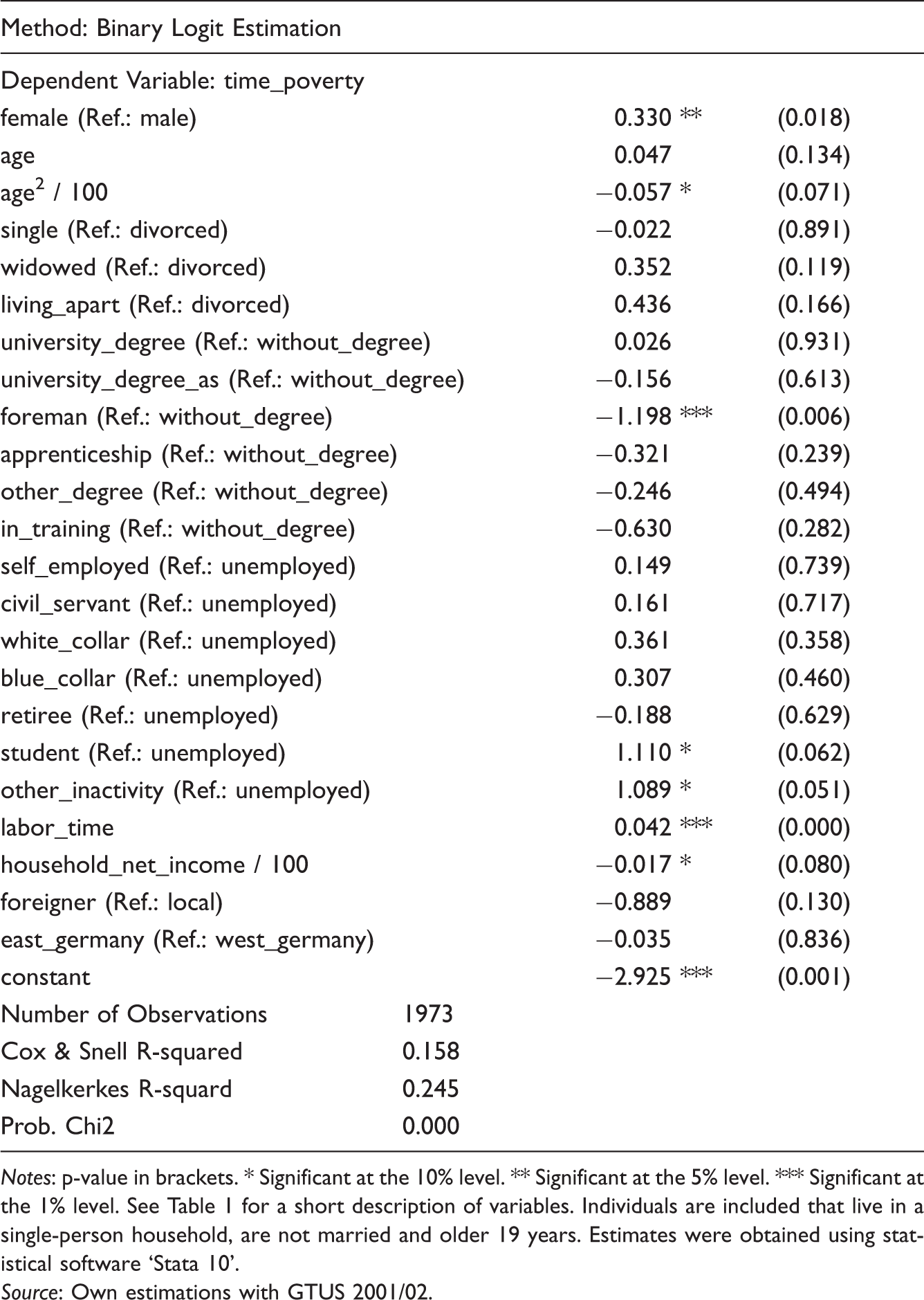
Notes: p-value in brackets. * Significant at the 10% level. ** Significant at the 5% level. *** Significant at the 1% level. See Table 1 for a short description of variables. Individuals are included that live in a single-person household, are not married and older 19 years. Estimates were obtained using statistical software ‘Stata 10’.
Source: Own estimations with GTUS 2001/02.
Imputation of the time poverty information from GTUS 2001/02 to IES 2003
Having the results of the binary logit estimation (see Table 2), the time–poverty–probability could be calculated for each individual in GTUS 2001/02 as well as in the IES 2003 since only explanatory variables are included that are present in both databases. 17 Confirming the well worked imputation process, relevant location and dispersion parameters of the time–poverty–probability in GTUS 2001/02 and in the EIES 2003 are close together (see Table 1). The average time–poverty–probability lies at 21.2% with standard deviation of 0.171 in GTUS 2001/02 and at 20.9% with standard deviation of 0.159 in the EIES 2003. 18 As described in the previous section, I judge those individuals time poor who have less than 60% median personal leisure time. In GTUS 2001/02, 21.2% are judged to be time poor. 19 It is obvious that a similar percentage of individuals should be judged to be time poor in the EIES 2003. Accordingly, the time–poverty–probability–threshold in the EIES 2003 is set at the time–poverty–probability of 37.5% to judge the same percentage of time poor as in GTUS 2001/02 with 21.2% of all individuals.20,21
Final estimations
OLS and 2SLQ estimations on the expenditure domain ‘communication services’.
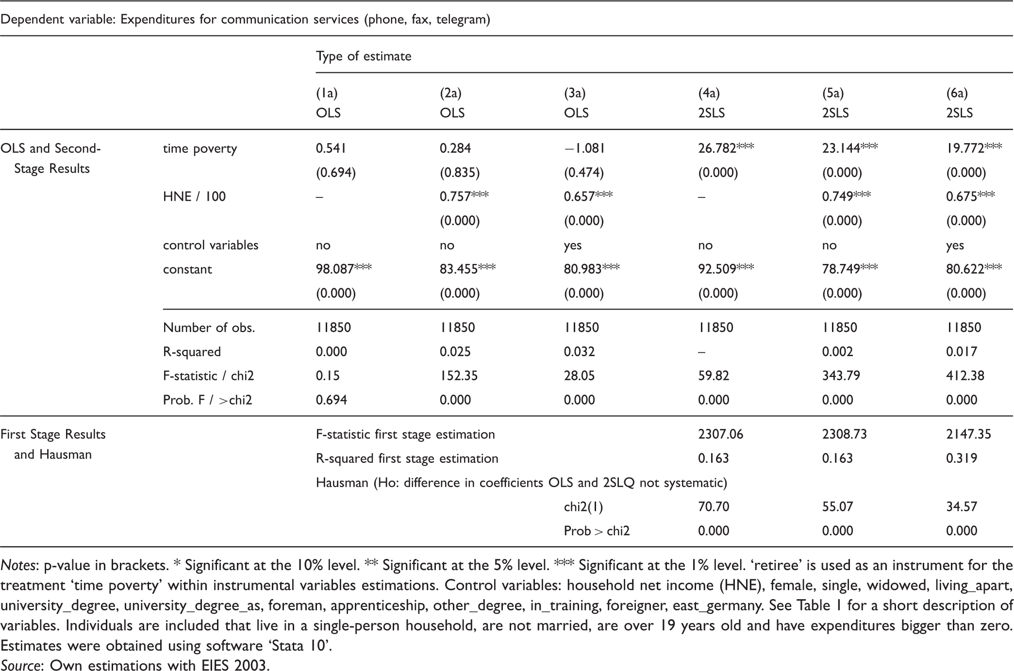
Notes: p-value in brackets. * Significant at the 10% level. ** Significant at the 5% level. *** Significant at the 1% level. ‘retiree’ is used as an instrument for the treatment ‘time poverty’ within instrumental variables estimations. Control variables: household net income (HNE), female, single, widowed, living_apart, university_degree, university_degree_as, foreman, apprenticeship, other_degree, in_training, foreigner, east_germany. See Table 1 for a short description of variables. Individuals are included that live in a single-person household, are not married, are over 19 years old and have expenditures bigger than zero. Estimates were obtained using software ‘Stata 10’.
Source: Own estimations with EIES 2003.
OLS and 2SLQ estimations on the expenditure domain ‘furniture’.

Notes: p-value in brackets. * Significant at the 10% level. ** Significant at the 5% level. *** Significant at the 1% level. ‘retiree’ is used as an instrument for the treatment ‘time poverty’ within instrumental variables estimations. Control variables: household net income (HNE), female, single, widowed, living_apart, university_degree, university_degree_as, foreman, apprenticeship, other_degree, in_training, foreigner, east_germany. See Table 1 for a short description of variables. Individuals are included that live in a single-person household, are not married, are over 19 years old and have expenditures bigger than zero. Estimates were obtained using software ‘Stata 10’.
Source: Own estimations with EIES 2003.
Expenditure domain ‘communication services’
Estimations on the first expenditure domain ‘communication services’ in Table 3 confirm our expected mechanism between time poverty and paid prices together with the expected bias in the OLS estimates primarily. The first estimation reports a significant constant together with a low and insignificant coefficient for the time poverty variable (OLS (1a)): If expenditures for ‘communication services’ exist, not time poor individuals spend in average 98.09 Euro for ‘communication services’ within 3 months while time poor individuals spend 98.63 Euro. 22 Controlling for household net income (divided by 100), the insignificant coefficient for time poverty decreases while the coefficient for household net income is statistically and economically significant (OLS (2a)): If household net income raises by 100 Euro, the expenditures for ‘communication services’ raise by 0.76 Euro. Controlling for further variables, the coefficient for household net income decreases slightly while the coefficient for time poverty remains insignificant (OLS (3a)).
As described in the previous section, I expect downward biased coefficients for the time poverty variable in the OLS estimations since the relevant and unobserved variable ability might be positive correlated with time poverty and paid prices per good. Instrumental variables estimations therefore are applied to clear bias in the time poverty coefficient using retiree as instrument for the treatment time poverty. F-statistics (>2147.35) together with the R-squareds (>0.16) of the first stage regression verifies retiree as strong instrument for time poverty (see Table 3). The Hausman Test confirms a systematic difference between OLS and 2SLS coefficients. Statistically and economically significant coefficients result for the time poverty variable using instrumental variables estimations (2SLS (4a) – (6a)). The time poverty coefficient decreases by controlling for household net income and further variables from 26.782 (2SLS (4a)) over 23.144 (2SLS (5a)) to 19.772 (2SLS (6a)), but remains statistically and economically significant: Time poor individuals spend in average 19.77 Euro more for ‘communication services’ than not time poor individuals within 3 months holding household net income and further control variables constant (2SLS (6a)).
Expenditure domain ‘care products’
OLS and 2SLQ estimations on the expenditure domain ‘hair care, shaving products, toilet paper’.

Notes: p-value in brackets. * Significant at the 10% level. ** Significant at the 5% level. *** Significant at the 1% level. ‘retiree’ is used as an instrument for the treatment ‘time poverty’ within instrumental variables estimations. Control variables: household net income (HNE), female, single, widowed, living_apart, university_degree, university_degree_as, foreman, apprenticeship, other_degree, in_training, foreigner, east_germany. See Table 1 for a short description of variables. Individuals are included that live in a single-person household, are not married, are over 19 years old and have expenditures bigger than zero. Estimates were obtained using software ‘Stata 10’.
Source: Own estimations with EIES 2003.
Expenditure domain ‘furniture’
Results for estimations on the third expenditure domain ‘furniture’ in Table 5 stand in contrast to the previous findings. Negative and significant coefficients for the time poverty variable in OLS estimations (OLS (1c) – (3c)) become more negative by applying instrumental variables estimations: If expenditures for ‘furniture’ exist, time poor individuals pay on average 264.50 Euro less than not time poor people within 3 months holding household net income and further control variables constant (2SLS (6c)).
Estimations on further expenditure domains – that are not reported within this article – present variable results, e.g. estimations on the expenditure domains ‘food products’, ‘auto liability insurances’, ‘barber services’, ‘TV’ or ‘fridges’: Most estimations point to positive and significant coefficients for the time poverty variable, some estimations present negative coefficients while some bring out insignificant coefficients. All in all, I do not find a positive, statistically and economically significant coefficient for the time poverty variable that is robust over the vast majority of expenditure domains and could certainly confirm our hypothesis Time poor individuals pay more for identical goods and services.
Discussion of findings
In ‘Data, empirical strategy, method and operationalisation’ section, requirements are formulated that must be met before applying an expenditure domain as dependent variable in the final estimations. The second requirement is: Time and not time poor individuals buy the same quality. There are empirical findings that question the fulfilment of this requirement by underlying the existence of a further mechanism: Although one might suggest that time poor individuals are rarely price conscious and therefore purchase branded articles more often, empirical findings point out that time rich individuals – who invest relatively more time into shopping – are more likely to purchase branded goods with a higher product quality (Wehner, 2004: 15). For example, the time poor individuals purchase at the discount store – half an hour before shop closing time – and accordingly pay less than time rich individuals who shop at wine and other specialty stores seeking advice from salespersons before deciding to purchase the high quality wine (Haller, 2004: 31). With EIES 2003 database, differences in product quality could not be identified. Only information about the sum of expenditures in different domains is available. This may be a source for misleading results.
Besides, the instrument retiree in the framework of instrumental variables estimation should have no partial effect on the outcome next to the indirect effect over the treatment variable time poverty. This assumption could be questioned: First, it may be that retirees have remarkably different consumption behaviour than younger individuals independent of their time poverty status. It might be plausible that typical not time poor retirees prefer high quality products and are willing to pay more than individuals of the younger generation (Precht, 2007: 333). Second, it is possible that people with a higher ability are more likely to retire later. Accordingly, the time poverty coefficient may be downward biased even in instrumental variables estimations. 23
The data used were collected from 2001 to 2003 by the Federal Statistical Office of Germany. The GTUS 2001/02 is still the latest available data including time use information. However, the manner of price search considerably changed since that time. Increasingly, the internet is used to compare prices of products and services within seconds. Websites and smartphone apps have specialised on price comparisons (e.g. www.hrs.com, www.pricegrabber.com). Price search will increasingly take less time, and accordingly, price dispersion will probably decline.
Concluding remarks
Within this article, I test whether time poor individuals compare less between prices as a result of their time deficit, therefore do not identify ‘bargains or rip-offs’ and pay in average more for identical products and services than not time poor individuals. Thereby, time use information is extracted from the GTUS 2001/02 and attached to the IES 2003 to identify time poor individuals in IES 2003. Instrumental variables estimations are arranged to account for an expected bias in OLS estimations – caused by the excluded variable (search) ability – and to catch the causal effect of time poverty on paid prices.
The findings do not show a consistent picture for different expenditure domains: A positive, statistically and economically significant coefficient for the time poverty variable that is robust over the vast majority of expenditure domains and which would confirm our hypothesis Time poor individuals pay more for identical goods was not found. Though two of the three reported estimations show the expected positive and significant coefficient for the time poverty variable (see the sixth estimation in Table 3 for the expenditure domain ‘communication services’ and Table 4 for the expenditure domain ‘hair care, shaving products, toilet paper’), one estimation presents negative coefficients (see the sixth estimation in Table 5 for the expenditure domain ‘furniture’), while further estimations (e.g. on the expenditure domains ‘food products’, ‘auto liability insurances’, ‘barber services’, ‘TV’ and ‘fridges’) – that are not reported within this paper – again produce variable results. Thus, a comprehensive mechanism that works well over the majority of the domains is not at hand. Accordingly, the stated hypothesis should be rather rejected. The effect of time poverty on the paid price seems to be dependent strongly on the inspected expenditure domain.
All in all, one should not assume that time poor individuals suffer large welfare losses according to the small amount of time spent comparing prices. One should rather suppose that time poor individuals find trust in stores at which they expect a fair price performance ratio (Haller, 2004: 31; Wehner, 2004: 15). For example, the time poor employed single father does not know the exact price for a litre of milk that is offered by different supermarkets, but he found trust in and remains faithful to a specific store which was convenient in the past (e.g. German discounter ‘ALDI’ or Swedish furniture store ‘IKEA’). Accordingly, the result suggest that time poor individuals do not invest much time into price search, but do nevertheless pay a similar amount for products and services than not time poor individuals – at least in certain expenditure domains.
Footnotes
Acknowledgements
I would like to thank Prof. Joachim Merz, Mirko Felchner (M.A.), Dr Dominik Hanglberger and Dipl.-Volksw. Rafael Rucha (Leuphana University Lüneburg, Research Institute on Professions (FFB)) for their valuable support as well as the participants of the 32nd annual meeting of the International Association for Time Use Research (IATUR), Sciences Po, Paris, France, July 7–10, 2010, and the participants of the EVS User Conference ‘Forschen mit dem Mikrozensus und der Einkommens- und Verbrauchsstichprobe’, Rheingoldhalle, Mannheim, Germany, September 29–30, 2011 for their helpful discussion.
Declaration of Conflicting Interests
The author declared no potential conflicts of interest with respect to the research, authorship, and/or publication of this article.
Funding
This research received no specific grant from any funding agency in the public, commercial, or not-for-profit sectors.