Jointly assessing multiple endpoints in pilot and feasibility studies

Abstract

Pilot and feasibility studies are routinely used to determine whether a definitive trial should be pursued; however, the methodologies used to assess feasibility endpoints are often basic and are rarely informed by the requirements of the planned future trial. We propose a new method for analyzing feasibility outcomes which can incorporate relationships between endpoints, utilize a preliminary study design for a future trial and allow for multiple types of feasibility endpoints. The approach specifies a Joint Feasibility Space (JFS) which is the combination of feasibility outcomes that would render a future trial feasible. We estimate the probability of being in the JFS using Bayesian methods and use simulation to create a decision rule based on frequentist operating characteristics. We compare our approach to other general-purpose methods in the literature with simulation and show that our approach has approximately the same performance when analyzing a single feasibility endpoint but is more efficient with more than one endpoint. Feasibility endpoints should be the focus of pilot and feasibility studies. The analyses of these endpoints deserve more attention than they are given, and we have provided a new, effective method their assessment.

Keywords

Pilot studies feasibility Bayesian analysis sample size

1 Introduction

Pilot and feasibility studies play an important role in research; they serve as proving grounds for ideas and when well-designed generate useful information for planning future randomized controlled trials (RCTs). These studies are ubiquitous, with a PubMed search for 2023 returning over 30,000 results for the terms “pilot study” or “feasibility study,” with no doubt many more studies that are unpublished. However, there has been a lack of clarity in the literature about the definition of, and differences between, pilot and feasibility studies. After conducting a Delphi study and literature review, Eldridge et al.¹ concluded that feasibility studies, which encompass pilot studies, are concerned with three questions: “whether something can be done, should we proceed with it, and if so, how?” To address these questions, feasibility studies collect many types of data, including estimates of preliminary efficacy, and measures of feasibility related to both the intervention and design of a future trial. Common feasibility measures focused on the intervention include acceptability to participants, demand for the intervention in the general population and related measures.² Feasibility endpoints related to the design of a future trial include recruitment rate, retention and measures of adherence. In our examples we focus on feasibility endpoints related to the design of a future trial, and specifically, how researchers can use these outcomes to inform their decision of whether to proceed to a larger trial, however, we note that our approach can incorporate measures related to the implementation as long as they are quantitatively assessed. For trials collecting multiple types of endpoints a mixed methods framework can be utilized with an overall decision on whether to proceed determined by if each part of the study was determined to be feasible.²

Despite the widespread use and importance of feasibility studies, their analysis plans are often basic. The Consolidated Standard of Reporting Trials (CONSORT) extension to pilot and feasibility studies³ identified the feasibility of a future RCT as the primary aim of a pilot study. Nevertheless, many studies continue to treat other endpoints, typically preliminary estimates of efficacy, as the primary endpoint. In a recent survey of pilots for cluster RCTs only 56% had feasibility as their primary outcome.⁴ Additionally, many pilot and feasibility studies use hypothesis testing of efficacy outcomes as their primary outcome; a 2010 survey found 81%⁵ of pilots used hypothesis tests and a more recent 2022 survey of one hundred pilots in rehabilitation research found 92% intended to evaluate efficacy with a hypothesis test.⁶ It is likely that researchers want to assess efficacy because those are the outcomes that are clinically meaningful. It is also possible that many researchers conducting early-stage studies do not have statistical support and may be most comfortable with hypothesis tests. Additionally, there has been a relative lack of methodological research concerning the best way to assess feasibility outcomes, or to determine an appropriate sample size for a pilot study based on feasibility outcomes, especially when there is more than one outcome driving “feasibility.” This combination of factors has contributed to basic methods being the norm in pilot and feasibility studies.

One of the most common approaches for assessing feasibility is to compare the outcome from each feasibility endpoint to a threshold, for example, comparing the observed retention rate to a predefined threshold of 0.80. Examples in recent articles using this approach abound: “Fidelity to the intervention manual at least 75% of activities in each session completed at a satisfactory/superior level”,⁷ “feasibility criteria were set …recruitment > 50% of available patients, dropouts < 20% …”,⁸ and “A proportion of 90% staying in the study is excellent, 80% is good (i.e. 20% drop-out).”⁹ One problem with this approach is that these thresholds are rarely calibrated for the future RCT, that is, there is no justification for why meeting a specific threshold would lead to a future trial being feasible. Instead, the thresholds are chosen based on results from previous studies, or simply values that are likely to appear appropriate to funding or regulatory reviewers, such as 80% or 90%. An additional problem is that a strict interpretation of these thresholds (and assuming an approximately symmetric sampling distribution for the statistics, which will be true for binomial endpoints with relatively small sample sizes) leads to a probability of determining a threshold was met of only ∼0.50 when the true feasibility parameter equals the threshold. This problem is exacerbated by multiple independent feasibility criteria. With m endpoints, the probability of all sample statistics meeting their thresholds is only ∼0.5 ^m even when the parameter values equal the thresholds. With m = 3 endpoints this probability is only 0.125 and Wilson et al.¹⁰ noted that the specific performance of a set of independent decision rules can vary dramatically depending on the specific thresholds chosen. While many studies propose this approach, we doubt it is strictly followed, instead researchers likely look for the feasibility endpoints to be “close” to their target values.

Avery et al.¹¹ proposed a variation of the threshold approach that explicitly defines what values are close enough. Their approach uses three tiers depending on the strength of the feasibility outcome: Red: Do not proceed, Amber: Potentially proceed based on possible trial improvements and Green: Proceed to a future trial. The method is referred to as a traffic light procedure and the decision is explicitly made if the point estimate falls in the Red or Green zone. If the estimate is in the Amber zone the decision depends on whether the study team believes this value can be improved in a subsequent trial (e.g. if retention missed the target rate, participant surveys might identify ways to improve retention). The adoption of this traffic light procedure has increased from 12% of trials surveyed in 2015 to 62% of trials surveyed in 2016¹² indicating a desire in the research community to better evaluate feasibility endpoints. The advantage of this approach, the Amber zone, is also its major limitation. The importance of the Amber zone rests on whether feasibility parameters can be improved which will not always be the case and there is concern that researchers may be optimistic in evaluating whether a criterion can be improved.

The traffic light procedure was further formalized by Lewis et al.¹³ as a combination of a point estimate and a hypothesis test. The decision to proceed in the Amber zone is based on a p-value. Specifically, the procedure requires the specification of the lower limit of the Green zone (G_LL) and the upper limit of the Red zone (R_UL). The Amber zone is split into Amber _R (major amendments, based on a p-value ≥ α) and Amber _G (minor amendment, p-value < α), where the p-value comes from either a binomial exact test or a normal approximation. All estimates in the Green zone as well as estimates in the Amber _G zone are treated as justifying proceeding to a future trial.

This approach was presented in terms of Type I error control and power; however, the method depends on both a point estimate, which is not constrained by the Type I error rate, and a hypothesis test, which is. If the null hypothesis is true, then the p-value is uniformly distributed so we will reject the null hypothesis 100·α % of the time regardless of the sample size or the hypothesized effect. However, the α level for the hypothesis test only governs whether to proceed in the Amber zone and therefore does not set an overall error rate for the decision rule. Notably, an incorrect decision to proceed can occur at a rate greatly exceeding α. For example, with N = 20, G_LL= 0.80, R_UL= 0.70, and α = 0.05 using the HT we would proceed if either (1) the point estimate, $\hat{p}$ is ≥ G_LL or (2) R_UL: < $\hat{p}$ < G_LL, and the p-value ≤ 0.05. Given a binomial random variable, with n = 20; π = 0.70 (i.e. the Null is true because π = R_UL) the probability of observing a sample mean of at least 0.80 (≥16 successes out of the 20 total) is 0.24. For this scenario, the AMBER zone consists of observing 15 successes, the only sample value such that 0.70 < $\hat{p}$ < 0.80. Using the binomial exact test to determine whether we should proceed in the Amber zone provides a p-value of 0.42. In this case, the HT procedure has error rate of 0.24, not 0.05, despite specifying α = 0.05.

In this paper, we propose a new method for assessing the feasibility of one or more quantitative endpoints. Our approach focuses on the probability that the set of feasibility measures are jointly feasible, and we compare our approach to other common methods both descriptively and using simulation. Notably, the method allows for trade-offs by incorporating functional relationships between multiple endpoints. We highlight this with examples including retention and recruitment rates, two of the most commonly collected feasibility endpoints. The motivation for the development of this method came from our experience designing pilot studies and attempting to create decision rules for multiple feasibility endpoints that had good operating characteristics, specifically a high probability of determining a future trial is feasible when it is and a low probability of determining a future trial is feasible when it is not.

2 Motivating example

We recently worked on the design of a pilot study for adults with Down syndrome (DS) and their caregivers. The intervention provides exercise sessions for the person with DS and counsels the caregiver in managing behavioral and neuropsychiatric symptoms associated with dementia, a common diagnosis in a person aging with DS. The study (KL2TR002367-08S1) is currently in pre-enrollment and will have co-primary aims, but for ease of the example we focus on only one, lessening the burden on the caregivers. In both the pilot and the future RCT the Modified Caregiver Strain Index (MCSI)¹⁴ will be used as the primary evaluation of caregiver burden. The pilot will recruit N = 20 caregivers and will be a 12-week intervention which mirrors the future RCT. The feasibility outcomes include recruitment and retention rate and our goal in designing the study was to have good operating characteristics for our decision based on these criteria.

The remainder of the manuscript is structured as follows, in Section 2 we discuss preliminary plans for a future trial and how this can lead to more realistic assessments of feasibility, in Section 3 we discuss Bayesian estimation of feasibility, and frequentist operating characteristics. In Section 4 we compare our approach to other methods and in Section 5 we summarize the proposed methodology. All simulations and plots were completed using R version 4.2.1 or higher¹⁵ and the code is available on GitHub.

3 Pre-planning and joint assessment

The questions a pilot study seeks to address (whether a future trial can be done, should we proceed, and if so, how?) depend on the specific future trial researchers hope to conduct. Consider a feasibility study with a stated goal of achieving at least 70% retention and a recruitment rate of 5 participants per month. An obvious, and typically unaddressed, question is why meeting or exceeding these thresholds would convince us that a future trial is feasible. When reasons are given for the thresholds, they are usually based on similarity to past trials. However, unless the planned RCT is extremely similar to the past trial, in required sample size, length of trial, participant burden, effectiveness, etc., there is little reason to believe we would need the same feasibility thresholds. Suppose the thresholds of 70% retention and 5 participants per month were based on what was achieved in a past RCT that targeted an intervention with an effect size of 0.50; if the intervention in a future RCT has a larger or smaller effect, then the thresholds will either be conservative or liberal because the required sample size will change. The only way to assess whether a future study will be feasible, is to have at least a rough outline of the planned design and required sample size depending on a set of assumptions (e.g. effect size, attrition rate, etc.). Then the feasibility of the assumptions that go into the design and power analysis of an RCT can be assessed using data from the pilot study. Outside of internal feasibility studies, developing a preliminary plan for a future RCT is rare but should be the standard for all feasibility trials. And even in internal pilot studies there is room for improvement in utilizing these plans to inform the pilot analyses; a 2019 review of 57 internal pilots funded by the National Institute for Health Care Research in the United Kingdom found that “while objectives were clear for the trials … none provided a specific rationale for choosing the progression criteria.”¹⁶ We believe a feasibility study cannot answer the questions it seeks to, unless the assessment of the feasibility endpoints is directly related to the planned future trial.

For our proposed pilot in patients with DS and their caregivers we conducted a preliminary design and power analysis for the planned RCT. The MCSI will be used to assess the impact on caregivers; however, there is no known clinically meaningful change in MCSI. Sorensen et al.¹⁷ conducted a meta-analysis on the effectiveness of interventions for caregivers and found that the effectiveness varied greatly depending on the type of intervention (e.g. Respite/daycare, Psychotherapy, etc.) with the smallest effect size of 0.01 and the largest of 0.62 (our proposed trial is similar to the interventions with larger estimated effects). For our examples, we proceed with a moderate effect size of δ = 0.22 and based on this we determined we would need approximately N = 165 participants to achieve 80% power with α = 0.05. Further, we assumed 80% retention, which increased our required sample to 207 participants. We then assumed a 36-month enrollment window for the full trial which would require average monthly enrollment of approximately 5.75 participants. Based on this preliminary plan we designed a pilot study to determine if it was feasible.

4 Relationships between pilot outcomes

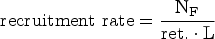
Multiple feasibility criteria are usually collected in pilot studies but are typically analyzed independently. Lewis at al. recently proposed a hypothesis test for feasibility parameters, and when discussing multiple outcomes proposed that “feasibility criteria should be considered separately, and hence overall progression would be determined by the worst-performing criterion.”¹³ While this approach may be reasonable in certain situations, even if it is likely conservative, there are situations where feasibility criteria are functionally related, and it would be appealing to directly incorporate these relationships. Two of the most frequently reported feasibility outcomes, recruitment, and retention rate, are related through the required sample size of a future trial. Given a preliminary sample size estimate for a future trial (N_F) assuming no attrition, an assumed retention rate (ret.) and an enrollment length (L), the required recruitment rate is given by the following formula:

recruitment rate = \frac{N_{F}}{ret . \cdot L}

This formalizes relationships that are well understood: as the retention rate increases, the required sample size decreases, which will lead to a lower required recruitment rate. Practically, this means that analyzing these two outcomes independently and focusing on the worst performing measure will lead to overly conservative progression rules. Returning to our pilot study example, we planned the pilot based on 80% retention, however, this was merely an assumption, and we will likely experience higher or lower retention in both our pilot and the future trial. We would certainly decide to proceed to a larger trial with better than assumed retention and we felt it would be acceptable to proceed with retention as low as 70%. Based on the previous formula, we can identify pairs of retention and recruitment rates that would be jointly feasible (i.e. the sample size required for the future trial would be achievable given the combination of retention and recruitment rate). Figure 1 shows the relationship between retention and recruitment rate to achieve 80% power and be able to fully enroll the study within 36 months. The shaded region represents the Joint Feasibility Space (JFS), and any pair of parameter values in the JFS indicates that the observed combination would lead to a future trial being feasible. Our preliminary plan was based on the assumed effect sizes for the MCSI which led to a preliminary sample size of N_F = 165 (with 100% retention). We assumed retention of ret. = 0.80 based on experience with this patient population and assumed an overall recruitment length of L = 36 months which requires 5.75 participants per month (rounded up from 5.73 to ensure an integer value for the number of participants). We can change either the recruitment rate or the retention rate to determine a new point on the boundary of the JFS. For example, if the true retention rate is worse than expected, for example, 70%, we would need the recruitment rate to be at least 6.56 participants per month, conversely, if observed retention is 90%, then a future trial would be feasible even if we can only recruit 5.1 participants per month.

Figure 1.

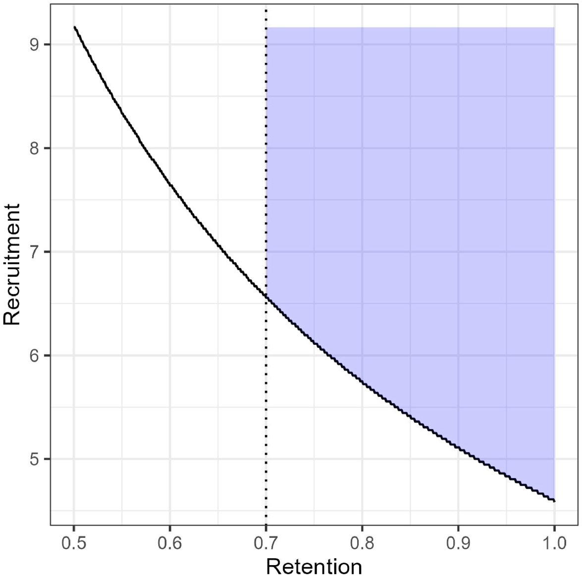
Joint feasibility space (JFS) for our proposed pilot constrained to require retention of at least 0.70.

While some parameter combinations might be feasible, they may not be acceptable either to the research team or to potential funders. A study with true retention rate of 50% and recruitment of 10 participants per month would indicate a future trial would be feasible, however, high attrition may indicate serious problems with the intervention that would limit its real-world efficacy. The JFS can be constrained based on these subjective reasons; Figure 1 shows the JFS constrained to require retention of at least 70% which is what we used in our study of DS patients and their caregivers. We also note that there is no requirement that feasibility criteria have a functional relationship, for example if we also measure acceptability (e.g. as a proportion) and wanted to proceed if the acceptability parameter were at least 0.70, that could be combined with our measures of retention and recruitment. The JFS in that case would be a quarter cylindrical shape in three dimensions (e.g. recruitment on the y-axis, retention on the x-axis, and acceptability on the z-axis).

5 Analyzing multiple feasibility measures using Bayesian methods and simulation

Let θ be a vector of feasibility parameters, for example θ = (θ_rec., θ_ret.), then we need to estimate Pr( θ ∈ JFS). If all endpoints are independent then the posterior joint probability is simply the product of the individual posterior probabilities, if they are not independent, then the joint probability can be estimated using simulation.

For our example, let θ_rec. and θ_ret. represent parameters for the recruitment and retention rate respectively, and let X_rec. and X_ret. be the corresponding counts of the participants recruited per month and binomial responses for retention. We want to estimate the posterior distribution $Pr (θ \in JFS | X_{rec .}, X_{ret .})$ . The individual posteriors Pr(θ_ret.|X_ret.) and Pr(θ_rec. | X_rec.) can be exactly determined using conjugate priors and then the joint posterior can be estimated using simulation. In most cases it is reasonable to assume that recruitment and retention rate are statistically independent, then pairs of values for recruitment and retention can be generated from their posterior distributions. The pairs are then compared to the JFS, with the estimated joint posterior probability calculated as the number of pairs inside the JFS divided by the total number of pairs. For recruitment rate we used a gamma prior and for retention rate a beta prior; the posterior distributions will then also be gamma and beta distributed, respectively. Both the beta and gamma distribution are defined by two shape parameters, Pr(θ_ret.) = Beta(α_β, β_β) and Pr(θ_rec.) = Gamma(α_γ, β_γ). The corresponding posterior distributions are then Pr(θ_ret | X_ret) = Beta(α_β + ∑X_ret, β_β + N−∑X_ret) and Pr(θ_rec | X_rec) = Gamma(α_γ + ∑X_rec, β_γ + NTR), where NTR stands for N to recruit, and is the number of weeks (months, years, etc.) needed to recruit such that N = ∑X_rec. For our pilot we plan to recruit N = 20 participants, thus the pilot will end when ∑X_rec= 20 and the number of weeks needed to recruit 20 caregivers will be NTR.

We will use weakly informative prior distributions for these examples; a Beta(α_β = 1, β_β = 1) for retention and Gamma(α_γ = 0.01, β_γ = 0.01) for recruitment. In Figure 2(a) and (b), the dashed line represents the prior distribution and, in both cases, the prior probability of meeting the feasibility threshold (≥0.80 retention rate, recruitment rate ≥ 5.75 per month) was low, only 0.20 and 0.04, respectively. However, these are weakly held prior beliefs that will be overwhelmed by the sample data. More informative prior distributions could be chosen, however, they run the risk of overwhelming the data when the sample is small, and it is questionable whether informative priors would be viewed favorably by reviewers.

Figure 2.

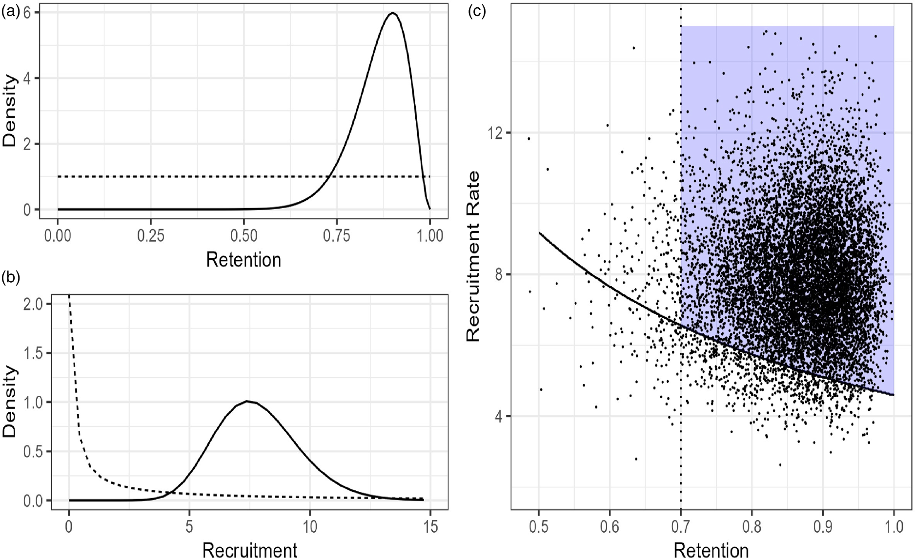
(a) Prior (dashed) and posterior (solid) distributions for Retention rate. (b) Prior and posterior distributions for Recruitment rate. (c) 10,000 draws from the joint posterior distribution overlaid on the JFS.

Given that our pilot has not been completed, we simulated hypothetical retention and recruitment data, shown in Table 1. We plan to enroll participants in cohorts and track the number of weeks of total active enrollment and convert this to a monthly rate. The simulated data in Table 1 shows it took 11 weeks, just over 2.5 months, to fully enroll the 20 participants, for a monthly recruitment rate of 7.9 participants per month. Recruitment data was simulated weekly with a rate parameter of 5.75/4.33, the posterior probability was calculated for weekly data and then converted to monthly. Data could have been simulated (or with real data, collected) as a monthly rate; however, the prior would be stronger in that case relative to the data and would need to be adjusted. We plan to calculate retention as the total number of individuals who complete both pre- and post-testing and for this simulated data set, we observed 18 out of 20 participants (90%) complete all visits.

Table 1.

Simulated feasibility data.

Feasibility endpoints	Simulated data	Summary statistics
Recruitment rate (weekly)	(1,2,1,3,3,0,1,3,1,1,4)	Monthly rate: 7.87
Retention rate	(1,1,1,1,1,1,0,1,1,1,1,0,1,1,1,1,1,1,1,1)	Retention rate: 0.90

To estimate the probability of being in the JFS, we generated pairs of observations from the joint posterior distribution and estimated the probability as the number of observations in the JFS divided by the total number of simulations (Figure 2(c)). With our simulated sample Pr(θ ∈ JFS) = 0.91, indicating a high probability that a future trial is feasible. This is notably different from taking the product of the individual posterior distributions for recruitment and retention rate, which would give an overly pessimistic probability of being in the JFS of 0.74. In this case, failing to incorporate the trade-offs between the two feasibility criteria has serious implications on the estimated probability a future trial is feasible. Another benefit of using the posterior probability is that it summarizes the evidence in favor of proceeding with a single value rather than requiring separate decision rules for each endpoint. In our example data, we have evidence of feasibility, and this probability could be used as the outcome of the pilot. However, in less clear-cut scenarios researchers would then need to subjectively decide if the Pr(θ ∈ JFS) = 0.91 (or 0.63, 0.78, etc.) is sufficient. Alternatively, we can define a probability cut point based on the operating characteristics it provides to avoid this subjective judgement.

6 Choosing a cut point based on two scenarios

We want to maximize the probability of proceeding when a future trial is feasible and minimize the probability when it is not. We propose to evaluate the observed probability of being in the JFS based on a cut point derived from frequentist operating characteristics. We will identify a cut point that will be exceeded at a high rate when a future trial is feasible and at as low a rate as possible when a future trial is infeasible.

Typically, the design of a definitive RCT rests on assumptions about a set of parameter values. For example, a submission for an RCT to a funding agency may specify assumptions for recruitment, retention, adherence, acceptability, etc. Based on these values, a specific sample size is required which drives many aspects of the trial, including timeline and budget. If these assumptions are met, then the trial should be sufficiently powered to assess its primary aim. We focus on the decision at this set of assumptions and denote the feasible set of parameters values as F and contrast it with an infeasible set of parameter values I.

Returning to our example, based on our preliminary power analysis, a feasible set of parameter values is given by F : (ret. = 0.80, rec. = 5.75), if the parameter values equal F, then the future trial will be feasible. The choice of I is subjective and any value not in the JFS would be acceptable, however, in practice we want I to be somewhat “close” to the JFS, so that we are not contrasting F with a meaningless competitor (e.g. if we let I : (ret. = 0.20, rec. = 1) finding a way to discriminate between these scenarios would be simple, but uninformative). Whenever possible I should also be informed by the future trial. For our future study, we will seek funding from the National Institutes of Health (NIH) for an R01 with an assumed recruitment window of 36 months. Therefore, we imagined the worst-case scenario as one where the required sample size (165 participants) is unattainable even with a no-cost-extension, that is, even if the recruitment window is extended from 36 to 48 months, we would still not fully recruit. Specifically, we assumed recruiting N = 164 participants (1 less than our target) at 48 months, a rate of 3.42 per month, which would result in only N = 123 participants being recruited at the end of the trial at 36 months (i.e. without an extension). If we use N = 123 in Equation 1 we specify a new curve which corresponds to a set of feasibility criteria satisfying these assumptions. Figure 3 shows this curve as a dotted line outside the JFS. We chose a point on this line close to F as our infeasible scenario; specifically, I : (ret. = 0.775, rec. = 4.42), denoted by a closed triangle. We also chose two other points along the curve (open triangles) as sensitivity analyses to the choice of I, they are I_S1 : (ret. = 0.85, rec. = 4.03) and I_S2 : (ret. = 0.70, rec. = 4.89).

Figure 3.

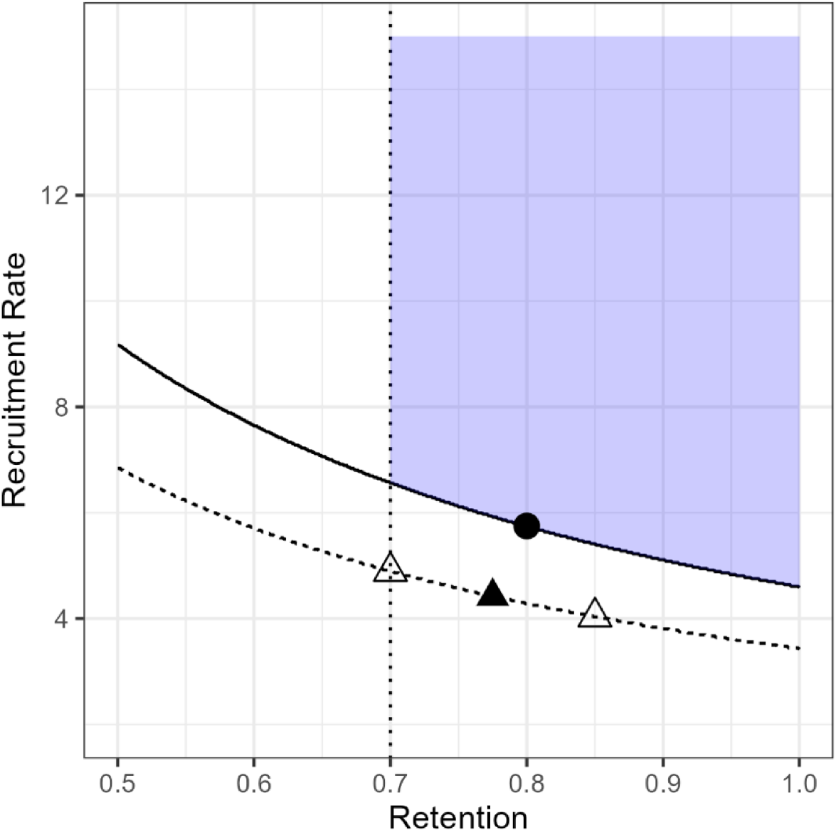
Condition F (closed dot), I (closed triangle), and I_S₁ and I_S₂ (open triangles).

Given these scenarios we can simulate pilot data sets with these characteristics and estimate the probabilities of being in the JFS. For each combination we generated 2000 unique data sets and for each data set estimated the joint posterior probability, allowing for trade-offs, with simulation. Given the small sample sizes and fact that condition F is only on the border of the JFS the overall probabilities are skewed toward 0; however, the sampling distribution of the posterior probabilities under F was much less skewed than the other conditions. The median probability for F was 0.32, while for I it was only 0.07. To achieve an 80% rate of proceeding conditional on F we identified a probability cut point of 0.10, that is, 80% of the estimated posterior probabilities from samples under condition F exceeded 0.10. Thus, in practice any estimated probability of being in the JFS that meets or exceeds this cut point would be taken as justifying proceeding to a larger trial. In the simulation this was met 41% of the time under condition I. In our example, the probability was not sensitive to the specific choice of I, for example the probability of exceeding the cut point for I_S1 was 0.39 and for I_S2 was 0.38. The results of a larger sensitivity analysis are presented in the Supplemental material.

If the operating characteristics of the decision rules are unacceptable then either the sample size can be increased or the distance between the F and I conditions can be increased, but these conditions should not be chosen simply to achieve specific probabilities of proceeding. For pilot studies with fixed sample sizes, such as our example, it allows us to identify the best operating characteristics that can be achieved with the resources available. A concern may be researchers’ hesitance to make a decision based on a low cut point despite having good operating characteristics. This could be addressed by requiring a lower probability of proceeding at F, for instance 50% based on this point being the minimum required combination, knowing that for any combination of parameter values farther inside the JFS we would have a higher probability of proceeding and the fact that this will result in a higher cut point. The operating characteristics a research team targets will depend on the specifics of their trial.

7 Comparing the JFS procedure to alternative methods

Our proposed approach to evaluating one or more feasibility criteria involves several steps and is listed here for reference:

Define the boundary of the JFS and prior distributions.

Define scenarios for when we should proceed (F) and should not proceed (I) for each endpoint.

Use simulation to identify a probability cut point to discriminate between F and I.

Assess sensitivity of the chosen points.

After data has been collected estimate Pr( θ ∈ JFS)

If Pr( θ ∈ JFS) ≥ cut point: proceed to a larger trial.

If Pr( θ ∈ JFS)< cut point: do not proceed to a larger trial.

For the simulation study we chose to focus only on proportions (e.g. retention rate) and to simulate the data from binomial distributions, and for multiple endpoints we simulated them independently. We did this for three reasons (1) many studies only include proportions as feasibility outcomes, even recruitment is often calculated as enrolled/screened with a target rate and we wanted to compare our procedure under this common scenario; (2) the hypothesis test method proposed by Lewis et al. can only include proportions and we wanted to include this method given its quick adoption in the research community (over 200 citations since being published in 2021); and (3) we did not include functional relationships between endpoints because this could bias the results in favor of our procedure.

We conducted two simulation studies. The first focused on a specific example which is similar to our pilot study and used retention values of F = 0.80, and I = 0.70 for one, two, and three feasibility endpoints. With two endpoints F = (0.80, 0.80) and I = (0.70, 0.70) and with three F = (0.80, 0.80, 0.80) and I = (0.70, 0.70, 0.70). We used N = 20, based on our example, and N = 119 because this was the stated sample size required to achieve power of 0.80 and a Type I error rate of 0.05 with the hypothesis test approach for the specified Red and Green zone limits of 0.70 and 0.80. For each combination of sample size and condition we simulated 5000 data sets. On each of these simulated data sets we used the proposed methods to determine if we would proceed to a future trial and then we took the mean across the 5000 results for each combination to estimate the probability of proceeding. Let Pr(P|C) denote the probability of proceeding (P) given a condition C = (F, I).

We compared our approach to three different methods, the threshold approach, an approach we refer to as the Tolerance method and the hypothesis test proposed by Lewis et al. The threshold approach specifies a target rate (T) for each endpoint and if the sample point estimate meets or exceeds the target $(\hat{p} \geq T)$ that part of the trial is considered feasible (for simplicity, in all examples and simulations we assume a larger value is better). For multiple endpoints, all feasibility criteria need to meet their thresholds. For example, target rates of 0.80 and 0.80 could be set for retention and adherence and the trial would be deemed feasible if the sample retention and adherence rates both exceeded 0.80.

Thresholds are routinely listed as part of a decision rule; however, we recognize that researchers will attempt to modify feasibility criteria that are close to the threshold and will therefore still choose to proceed even if the threshold is not strictly met. The tolerance method we propose is an attempt to formalize this common practice. We specify a threshold but will proceed if ( $\hat{p} \geq T - δ$ ), where we define $δ$ as the allowable tolerance. For example, if we set a target of T = 0.80, with $δ = 0.05$ , then any observed point estimate ≥ 0.75 will be considered feasible. Before conducting the simulation, we identified tolerances such that $Pr (P | F) \geq 0.80$ , that is, we will proceed 80% of the time when we should. With N = 20, and T = 0.80 the tolerance was set at 0.05 ( $T - δ$ = 0.75) because if X is a binomial random variable (n = 20, π = 0.80) then $Pr (X \geq 15) = 0.804$ , which is the smallest number of successes that achieves a probability of at least 0.80. Supplemental Table S1 provides the tolerances for all combination in the simulation study.

The final comparator was the hypothesis test proposed by Lewis et al.¹³ For each endpoint the researcher specifies a “Green lower limit” (G_LL) and a “Red upper limit” (R_UL). A point estimate ≥ G_LL indicates feasibility and a value ≤ R_UL indicates infeasibility. Point estimates between R_UL and G_LL are in the “Amber zone” and Lewis et al. proposed deciding to proceed if the p-value for a binomial test was ≤ α. For our simulations we varied the α level to attain $Pr (P | F) \geq 0.80$ , the values for α are provided in Supplemental Table S2. For multiple endpoints Lewis et al. proposed the α level should be unchanged, but the power of the tests should be modified to retain a desired power across all endpoints. For two endpoints with a desired power of 0.80 the authors suggested using power of $\sqrt{0.80} = 0.89$ for each endpoint while keeping $α = 0.05$ . The authors stated that no multiplicity correction would be needed for $α$ because to proceed each endpoint would need to be deemed feasible. However, we have found that this method performs poorly for multiple endpoints and used a simple adjustment that performs better. We adjusted the $α$ level of each endpoint to be $\sqrt[m]{α}$ , where m is the number of endpoints, for example, rather than maintaining $α = 0.05$ for two endpoints we use $α = 0.22$ , for the same reason we adjusted the power, that to incorrectly proceed we would need to incorrectly proceed on all outcomes. The results in Table 3 (second simulation study) are based on this adjustment which performs much better than the original method.

Table 2.
Comparison of JFS with other methods.

Endpoints Sample size Condition Threshold Tolerance JFS (Tol) HT JFS (HT)

1 20 I 0.24 0.43 0.43 0.43 0.43

F 0.62 0.80 0.80 0.80 0.80

119 I 0.005 0.05 0.05 0.05 0.05

F 0.48 0.80 0.80 0.80 0.80

2 20 I 0.06 0.39 0.38 0.19 0.19

F 0.41 0.83 0.87 0.65 0.71

119 I 0.00 0.01 0.01 0.01 0.01

F 0.23 0.82 0.87 0.82 0.87

3 20 I 0.01 0.47 0.46 0.07 0.08

F 0.25 0.91 0.95 0.51 0.62

119 I 0.00 0.003 0.002 0.003 0.002

F 0.12 0.82 0.93 0.82 0.93

Endpoints	Sample size	Condition	Threshold	Tolerance	JFS (Tol)	HT	JFS (HT)
1	20	I	0.24	0.43	0.43	0.43	0.43
F	0.62	0.80	0.80	0.80	0.80
119	I	0.005	0.05	0.05	0.05	0.05
F	0.48	0.80	0.80	0.80	0.80
2	20	I	0.06	0.39	0.38	0.19	0.19
F	0.41	0.83	0.87	0.65	0.71
119	I	0.00	0.01	0.01	0.01	0.01
F	0.23	0.82	0.87	0.82	0.87
3	20	I	0.01	0.47	0.46	0.07	0.08
F	0.25	0.91	0.95	0.51	0.62
119	I	0.00	0.003	0.002	0.003	0.002
F	0.12	0.82	0.93	0.82	0.93

HT: hypothesis test proposed by Lewis et al.; JFS (Tol): The JFS procedure with Pr(P|I) matched to the tolerance approach; JFS (HT): JFS procedure with Pr(P|I) matched to HT.

Table 3.

Relative efficiency of the JFS compared to the hypothesis test proposed by Lewis et al.

		One endpoint	Two endpoints	Three endpoints
I	F	N (RE)	N (RE)	N (RE)
0.1	0.2	78 (1.00)	44 (0.79)	31 (0.66)
0.15	0.25	101 (1.00)	52 (0.76)	42 (0.74)
0.15	0.30	48 (1.00)	25 (0.76)	17 (0.55)
0.20	0.30	116 (1.00)	64 (0.81)	52 (0.78)
0.20	0.35	56 (1.00)	29 (0.76)	21 (0.64)
0.20	0.40	35 (1.00)	17 (0.71)	12 (0.63)
0.25	0.35	129 (1.00)	74 (0.83)	58 (0.79)
0.25	0.40	62 (1.00)	33 (0.80)	23 (0.61)
0.25	0.45	36 (1.00)	20 (0.77)	13 (0.59)
0.25	0.50	26 (1.00)	12 (0.75)	9 (0.60)
0.30	0.40	144 (1.00)	84 (0.85)	62 (0.81)
0.30	0.45	67 (1.00)	34 (0.70)	24 (0.63)
0.30	0.50	39 (1.00)	21 (0.75)	14 (0.64)
0.30	0.55	25 (1.00)	14 (0.74)	10 (0.77)
0.30	0.60	17 (1.00)	9 (0.82)	6 (0.60)
0.35	0.45	148 (1.00)	86 (0.84)	65 (0.81)
0.35	0.50	68 (1.00)	37 (0.77)	25 (0.66)
0.35	0.55	41 (1.00)	21 (0.78)	14 (0.64)
0.35	0.60	26 (1.00)	14 (0.82)	9 (0.64)
0.35	0.65	19 (1.00)	10 (0.83)	6 (0.55)
0.40	0.50	158 (1.00)	89 (0.86)	70 (0.82)
0.40	0.55	71 (1.00)	37 (0.82)	26 (0.63)
0.40	0.60	42 (1.00)	22 (0.79)	15 (0.63)
0.40	0.65	28 (1.00)	13 (0.76)	10 (0.63)
0.40	0.70	19 (1.00)	9 (0.64)	6 (0.60)
0.45	0.55	154 (1.00)	95 (0.86)	69 (0.82)
0.45	0.60	70 (1.00)	37 (0.77)	26 (0.62)
0.45	0.65	42 (1.00)	21 (0.72)	15 (0.65)
0.45	0.70	25 (1.00)	14 (0.82)	9 (0.69)
0.45	0.75	16 (1.00)	8 (0.62)	6 (0.55)
0.50	0.60	158 (1.00)	88 (0.85)	74 (0.83)
0.50	0.65	69 (1.00)	36 (0.73)	25 (0.71)
0.50	0.70	37 (1.00)	21 (0.84)	14 (0.67)
0.50	0.75	23 (1.00)	14 (0.74)	9 (0.60)
0.55	0.65	150 (1.00)	86 (0.85)	68 (0.82)
0.55	0.70	70 (1.00)	36 (0.80)	24 (0.65)
0.55	0.75	37 (1.00)	21 (0.91)	13 (0.62)
0.60	0.70	143 (1.00)	78 (0.84)	60 (0.80)
0.60	0.75	62 (1.00)	32 (0.80)	22 (0.65)
0.60	0.80	36 (1.00)	18 (0.75)	12 (0.63)
0.65	0.75	133 (1.00)	74 (0.83)	57 (0.79)
0.65	0.80	55 (1.00)	29 (0.78)	20 (0.67)
0.65	0.85	31 (1.00)	17 (0.81)	10 (0.67)
0.70	0.80	119 (1.00)	64 (0.81)	48 (0.76)
0.70	0.85	49 (1.00)	26 (0.81)	18 (0.76)
0.75	0.85	103 (1.00)	53 (0.82)	36 (0.71)
0.75	0.90	45 (1.00)	22 (0.88)	15 (0.71)
0.80	0.90	82 (1.00)	44 (0.81)	29 (0.67)
Mean RE		1.00	0.79	0.68

The decision rules for each approach are:

Threshold: Proceed if point estimate ≥ 0.80 on all endpoints

Tolerance: Proceed if point estimate ≥ 0.80− $δ$ on all endpoints

Hypothesis test: Proceed if point estimate ≥ 0.80 (G_LL) or point estimate ≥ 0.70 (R_UL) and p-value < α on all endpoints.

JFS: Proceed if estimated Pr(θ ∈ JFS) ≥ cut point.

The threshold, tolerance, and hypothesis test methods cannot always achieve the specified performance, that is,

Pr (P | F) \geq 0.80

. For ease of comparison, we matched the JFS

Pr (P | I)

to the

Pr (P | I)

for the tolerance and hypothesis test method, which are referred to in the table as JFS (Tol) and JFS (HT). Then to determine which method is better we can simply compare the

Pr (P | F),

with the higher value indicating better performance.

The simulation results are presented in Table 2. As expected, the Threshold approach performed poorly; despite a strict threshold being reported in many pilot and feasibility studies we doubt they are rigorously enforced, and this simulation provides further evidence that they should not be. The only advantage of the Threshold procedure is that it has the best control of proceeding when we should not; however, in early-stage studies a higher rate of erroneously proceeding is typically accepted given that tight control of this error rate would lead to effective interventions being abandoned early. The tolerance and hypothesis test approaches have similar, often identical, operating characteristics. In the sample size and effect combinations we examined this was because of the discreteness of the underlying binomial random variable. For example, with N = 20, and an effect of 0.80 the tolerance was set to 0.05, which corresponds to 15 out of 20 subjects meeting the criteria. For the hypothesis test, we checked different values of α and found that letting α = 0.42 was the smallest level we could set to achieve Pr(P|F) ≥ 0.80. The p-value for a binomial test will be less than 0.42 when there are at least 15 successes out of the 20 subjects, so these two approaches proceed in the same situations. The only time the tolerance and hypothesis test approach differed in our simulations was when it was impossible for the hypothesis test to achieve Pr(P|F) ≥ 0.80. For example, with N = 20 and two feasibility endpoints the probability of both estimates exceeding the R_UL with a binomial n = 20 and $π$ = 0.80 is only 0.65, thus, the α level does not matter, and for these simulations we set α = 1.0. This seems to be an advantage of the tolerance approach over the hypothesis test, it can attain the desired probabilities of proceeding in a wider range of settings.

For a single endpoint, the three measures have approximately identical operating characteristics; however, as the number of feasibility endpoints increased so did differences in performance. With two feasibility endpoints we were able to match the Pr(P|I) for both the tolerance and hypothesis test methods while achieving a higher Pr(P|F). This same pattern held with three endpoints, with the JFS procedure achieving much better operating characteristics. For multiple binomial feasibility endpoints, the JFS procedure has better performance than these other methods.

To determine whether these results would hold in more general settings, we conducted another simulation study to estimate the required sample size to achieve specific progression probabilities. Table 3 shows the combinations of F and I that we considered, these are the same combinations that Lewis et al. provided sample sizes for. For each combination we considered one, two, and three feasibility endpoints as in the previous simulation and restricted ourselves to binomial endpoints. In these simulations we only compared the hypothesis test procedure to the JFS and focused on the sample size required to achieve Pr(P|F) = 0.80 and Pr(P|I) = 0.05. The required sample sizes for the hypothesis test approach using the binomial exact test were calculated using G*Power version 3.1,¹⁸ as in the original paper.

We used the JFS_N function described in the Supplemental material and available on GitHub, with 10,000 simulated unique data sets to approximate the sample sizes needed for the JFS procedure. Let N_JFS and N_HT be the required sample sizes for the JFS and hypothesis test procedure, then we defined the relative efficiency RE as $\frac{N_{J F S}}{N_{H T}}$ , thus, an RE < 1 indicates better efficiency for the JFS procedure. Given the similar performance with one endpoint in Table 2, in these simulations for one feasibility endpoint we assessed whether the JFS procedure was able to match the hypothesis test in required sample size. For all combinations of F and I we found this was true with RE = 1 across all combinations. With two and three endpoints the required sample sizes were significantly less than the hypothesis test approach across every combination of F and I. For two endpoints the average RE was 0.79, and for three endpoints was 0.68, indicating the JFS procedure requires far fewer observations than the approach proposed by Lewis et al. for multiple endpoints.

8 Discussion

Well-conducted pilot studies are critical to ensure that follow-up trials are feasible. Commonly used methods for assessing feasibility criteria are often simplistic and fail to account for potential relationships between the outcomes. These issues can lead to poor decision making at the end of a feasibility study. In this manuscript, we have presented a new procedure to assess multiple, possible related, feasibility endpoints. Through simulations we have shown that our procedure outperforms widely used alternative methods by achieving a higher probability of proceeding when we should while maintaining an equivalent probability of proceeding when we should not in specific examples and showed that in general our procedure is more efficient than the hypothesis test approach. A key advantage of the JFS procedure is that it allows for specific functional relationships between two or more feasibility criteria, these simply change the boundaries of the feasibility space and additional relationships beyond retention and recruitment can be incorporated if they exist. An additional advantage of our approach is the ability to include feasibility endpoints of many types, for example, proportions, rates, means, etc., without requiring specific combinations of endpoints. We have provided sample size estimates for one, two, and three binomial feasibility endpoints for many combinations of F and I and have provided code to calculate a cut point and estimate a sample size for any number of binomial endpoints and/or a measure of recruitment rate.

A key limitation of this study is that other methods have been proposed that were not included in the simulation studies. Wilson et al.¹⁹ proposed a Bayesian decision theoretic approach based on the traffic light procedure that allowed for trade-offs between acceptable error rates for incorrect decisions (e.g. choosing not to proceed when the parameter is in the green zone). This approach was shown to have good performance. However, it is computationally expensive, and it requires the specification of a loss function (a piecewise loss function was used in the examples). The elicitation of a loss function is a difficult, and often unfamiliar, problem, and this is likely to be exacerbated in the setting of a pilot study. Another interesting method proposed by Wilson et al.¹⁰ constructed a hypothesis test based on the power of a future trial for pilot studies collecting recruitment, adherence and follow-up rates (what we have called retention), and was extended to incorporate estimation of the standard deviation. The hypothesis test also incorporated an assumed relationship between adherence and effectiveness and allowed for randomness of recruitment and observation in defining the power and operating characteristics of the future trial. The major limitation of this approach, and the reason it was not included in the simulation studies is that it is only applicable for a pilot study collecting a subset of recruitment, adherence and follow-up rates as the feasibility endpoints. These are common feasibility outcomes; however, pilot studies collect many types of endpoints, including measures of acceptability, safety, compliance, cost and others. A cursory look at published pilot studies will show that it is uncommon for the key feasibility criteria to only include a subset of recruitment, retention, and adherence. Our proposed method is meant to be a general solution and can incorporate as many endpoints as needed, and these can be rates, counts, proportions etc. In our simulations we chose to focus on comparing our method to another general-purpose solution, the hypothesis test from Lewis et al. However, the hypothesis test from Wilson et al. may be more appropriate for trials that collect a subset of recruitment, adherence, and follow-up rates. Further simulation studies would be needed to compare the operating characteristics of our proposed approach to the test proposed by Wilson et al. or other methods under specific scenarios.

Another limitation of our approach is the computational complexity. A probability cut point must be defined, based on simulation, and outside of simple scenarios the posterior probability of θ being in the JFS must be estimated using simulation as well. Additionally, there is no closed-form solution for the sample size, and simulation must be used to estimate the required sample. We have provided code to calculate the required cut points for scenarios with all binomial data, or where recruitment data is also included. We have also provided code to approximate the sample size if all feasibility endpoints are binomially distributed; however, combinations of endpoints of various types will require simulations tailored to those conditions, and while we have provided example code on GitHub that can serve as a starting point this may be beyond the skillset of some study teams. Another limitation is the subjective choice of the conditions, especially I, however, the impact of this choice can be assessed using sensitivity analyses.

We note that some of the required sample sizes in Table 3 are extremely small, and even though the simulations showed good operating characteristics we would not feel confident in the results from a pilot with N = 6 and three feasibility endpoints (row 15 in Table 3, I = (0.30, 0.30, 0.30) and F = (0.60, 0.60, 0.60)). These small sample sizes are driven by extreme differences between the F and I conditions. In general, the specification of F and I will be unfamiliar to many researchers. While these choices are subjective, we would encourage researchers to limit the distance between F and I such that the I condition is as close to feasible as possible. As an example, for our pilot study we chose F = 0.80 for retention; the operating characteristics of our approach would have been excellent had we chosen I = 0.50, but the ability to discriminate between these two scenarios is not meaningful. Sensitivity analyses, such as those shown in Figure 3 (and the Supplemental material), should be undertaken to determine whether the operating characteristics of the method are highly depending on the choice of F, and especially I. Another consideration for researchers is that with a fixed sample size, as the number of endpoints increases the probability that all of them will be in the JFS will quickly decrease. For specific scenarios the probability, especially under condition I, will approach 0 and either the sample size or the number of simulated data sets would need to increase to accurately estimate this value. (Or more hopefully, researchers will be confronted by the inability of any method to adequately assess many endpoints with small sample sizes.) Our provided code will give an error if the only probability cut point identified is 0. In the Supplemental material we describe the R functions to approximate the sample size and identify the probability cut point. We believe the JFS procedure provides a meaningful and efficient way to analyze multiple feasibility outcomes that can be used in very general settings.

Supplemental Material

sj-docx-1-smm-10.1177_09622802241311219 - Supplemental material for Jointly assessing multiple endpoints in pilot and feasibility studies

Supplemental material, sj-docx-1-smm-10.1177_09622802241311219 for Jointly assessing multiple endpoints in pilot and feasibility studies by Robert N Montgomery, Amy E Bodde and Eric D Vidoni in Medical Research

Footnotes

Acknowledgements

We thank the reviewers for their helpful comments and corrections which have sharpened the focus and clarity of this manuscript.

Declaration of conflicting interests

The authors declared no potential conflicts of interest with respect to the research, authorship, and/or publication of this article.

Funding

The authors disclosed receipt of the following financial support for the research, authorship, and/or publication of this article: This work was supported in part by the National Institute on Aging of the National Institutes of Health under award number R03AG073932. The content is solely the responsibility of the authors and does not necessarily represent the official views of the National Institutes of Health.

ORCID iD

Robert N Montgomery

Supplemental material

Supplemental material for this article is available online.

References

Eldridge

Lancaster

Campbell

, et al. Defining feasibility and pilot studies in preparation for randomised controlled trials: development of a conceptual framework. PLoS One 2016; 11: e0150205.

Bowen

Kreuter

Spring

, et al. How we design feasibility studies. Am J Prev Med 2009; 36: 452–457.

Eldridge

Chan

Campbell

, et al. CONSORT 2010 statement: extension to randomised pilot and feasibility trials. Bmj-Brit Med J 2016; 355.

Chan

Leyrat

Eldridge

. Quality of reporting of pilot and feasibility cluster randomised trials: a systematic review. Bmj Open 2017; 7.

Arain

Campbell

Cooper

, et al. What is a pilot or feasibility study? A review of current practice and editorial policy. Bmc Med Res Methodol 2010; 10.

Lawson

Mellor

Eddy

, et al. Pilot and feasibility studies in rehabilitation research A review and educational primer for the physiatrist researcher. Am J Phys Med Rehab 2022; 101: 372–383.

Rose-Clarke

Rimal

Morrison

, et al. Development and testing the feasibility of a sports-based mental health promotion intervention in Nepal: a protocol for a pilot cluster-randomised controlled trial. Pilot Feasibility St 2023; 9.

Karlsson

Nygren-Bonnier

Henningsohn

, et al. The feasibility of using a digital tool to enhance mobilisation following abdominal cancer surgery-a non-randomised controlled trial. Pilot Feasibility St 2023; 9.

van de Winckel

Carpentier

Deng

, et al. Using remotely delivered Spring Forest Qigong™ to reduce neuropathic pain in adults with spinal cord injury: protocol of a quasi-experimental feasibility clinical trial. Pilot Feasibility St 2023; 9.

10.

Wilson

Brown

Farrin

, et al. A hypothesis test of feasibility for external pilot trials assessing recruitment, follow-up, and adherence rates. Stat Med 2021; 40: 4714–4731.

11.

Avery

KNL

Williamson

Gamble

, et al. Informing efficient randomised controlled trials: exploration of challenges in developing progression criteria for internal pilot studies. Bmj Open 2017; 7.

12.

Herbert

Julious

Goodacre

. Progression criteria in trials with an internal pilot: an audit of publicly funded randomised controlled trials. Trials 2019; 20.

13.

Lewis

Bromley

Sutton

, et al. Determining sample size for progression criteria for pragmatic pilot RCTs: the hypothesis test strikes back!. Pilot Feasibility St 2021; 7.

14.

Thornton

Travis

. Analysis of the reliability of the modified caregiver strain index. J Gerontol B-Psychol 2003; 58: S127–SS32.

15.

Team RC. R: A Language and Environment for Statistical Computing. 2023.

16.

Rosala-Hallas

Gamble

Blazeby

, et al. A review of current practice in the design and assessment of internal pilots in UK NIHR clinical trials. Trials 2019; 20.

17.

Sorensen

Pinquart

Duberstein

. How effective are interventions with caregivers? An updated meta-analysis. Gerontologist 2002; 42: 356–372.

18.

Faul

Erdfelder

Lang

, et al. G*power 3: a flexible statistical power analysis program for the social, behavioral, and biomedical sciences. Behav Res Methods 2007; 39: 175–191.

19.

Wilson

Wason

JMS

Brown

, et al. Bayesian design and analysis of external pilot trials for complex interventions. Stat Med 2021; 40: 2877–2892.

Supplementary Material

Please find the following supplemental material available below.

For Open Access articles published under a Creative Commons License, all supplemental material carries the same license as the article it is associated with.

For non-Open Access articles published, all supplemental material carries a non-exclusive license, and permission requests for re-use of supplemental material or any part of supplemental material shall be sent directly to the copyright owner as specified in the copyright notice associated with the article.

0.00 MB

0.21 MB