
Abstract
In clinical studies, the illness-death model is often used to describe disease progression. A subject starts disease-free, may develop the disease and then die, or die directly. In clinical practice, disease can only be diagnosed at pre-specified follow-up visits, so the exact time of disease onset is often unknown, resulting in interval-censored data. This study examines the impact of ignoring this interval-censored nature of disease data on the discrimination performance of illness-death models, focusing on the time-specific area under the receiver operating characteristic curve in both incident/dynamic and cumulative/dynamic definitions. A simulation study with data simulated from Weibull transition hazards and disease state censored at regular intervals is conducted. Estimates are derived using different methods: the Cox model with a time-dependent binary disease marker, which ignores interval-censoring, and the illness-death model for interval-censored data estimated with three implementations—the piecewise-constant model from the
Introduction
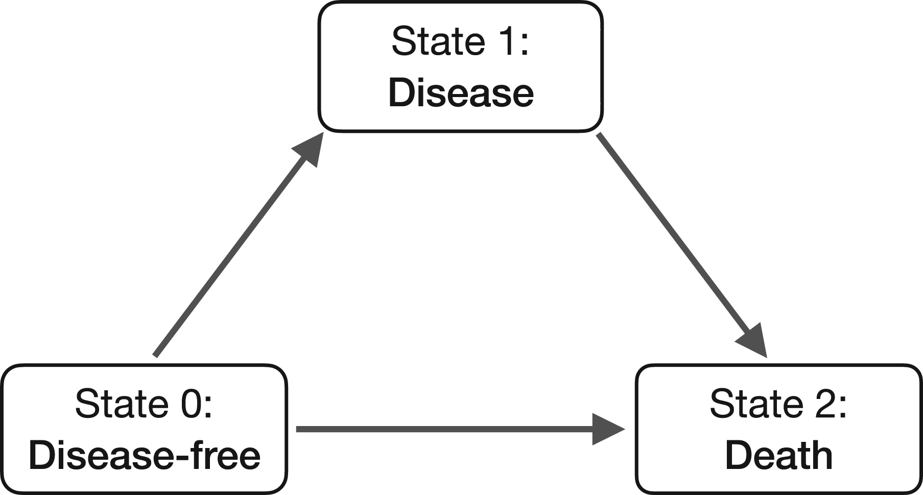
Survival analysis studies the distribution of time from an origin event to an event of interest. 1 It is often applied in the medical field where for example the time from diagnosis to death is studied. The intrinsic peculiarity of survival data is that they are generally incomplete: the event of interest cannot always be observed because it takes time to observe it. Data of individuals who did not experience the event of interest within a specific time window are hence right-censored. A frequently used method to study the effect of covariates on survival time is the Cox proportional hazards model. 2 In the medical field, it is often applied to study the effect of risk factors on a single event such as death or disease progression. However, in practice disease progression may be described by more than one type of event. These more complex event structures can be modeled simultaneously using multi-state models.3–5 The most simple of such models is the illness-death model, which is described by three states (see Figure 1): an individual is initially disease-free (state 0), he may then develop disease (state 1) and die (state 2) or he may die without disease. Like in the single event situation, the Cox model can be used to model the effect of covariates on the transitions between states.
Illness-death model.
The illness-death model is applicable to a variety of disease settings; a problem arises, however, if the time of disease cannot be observed exactly. Often, disease can only be diagnosed at pre-specified follow-up times. An example lies in the care of patients with soft tissue sarcoma. After initial treatment by tumor removal surgery a patient may first develop distant metastases and then die. Metastases are diagnosed at pre-specified follow-up visits at which an X-ray of the patient is screened. If metastases are found, it is therefore only known that they appeared between the last negative screening and the first positive screening. This peculiar disease data contains two types of missing information: (1) the time of disease onset is only known to have happened between two visits, that is, it is interval-censored; (2) if the last disease screening prior to death or last recorded follow-up was negative the disease status of a patient between last screening and death or last recorded follow-up is unknown.
The illness-death model for interval-censored data has been previously studied.4,6 It was found that ignoring the observation scheme of the data leads to biased estimates of regression coefficients, baseline hazards, and survival rates. A prominent motivation to illness-death model for interval-censored disease data comes from the study of dementia data.7–12 Dementia is diagnosed at infrequent follow-up visits which results in the time to dementia being interval-censored. Further, if a patient’s last dementia test was negative and he dies, it is not known if he acquired dementia prior to death. Frydman 7 developed a non-parametric maximum likelihood procedure for the estimation of the cumulative transition hazards when times of disease are interval-censored. Here, the second form of incompleteness was not addressed, as the author assumed that the disease state is known before death or right-censoring time. Joly et al. 8 proposed a non-parametric penalized likelihood method to estimate transition intensities in an illness-death model with an intermittently observed disease state. Simulations showed that not adjusting for the interval-censored nature of the data leads to a systematic bias in the estimation of transition intensities. Frydman and Szarek 9 extended the Frydman’s methodology 7 to incorporate the observations with unknown intermediate event status. They estimated the distribution of the time to the first occurrence of disease or death and showed that their method corrects bias. Yu et al. 10 used multiple imputation to analyze two aspects concerning the risk of dementia: the risk of developing dementia and the impact of dementia on survival. Leffondré et al. 11 performed simulation studies to show how interval-censoring affects the estimation of the effect of risk factors. More recently, Sabathé et al. 12 extended the pseudo-value approach 13 to interval-censored data in an illness-death model by using a semi-parametric estimator based on penalized likelihood approximated by splines. This extension allowed for the direct estimation of the impact of covariates on the probability of staying alive and non-demented, on the absolute risk, and on the restricted mean survival time without dementia.
In the R software,
14
illness-death models with exactly observed event times can be estimated with several R-packages, such as the
While the effect of ignoring the interval-censored nature of the disease data on regression coefficients and baseline hazards has been studied,4,6 its impact on the assessment of predictive performance has been neglected so far. The predictive performance of a model can be evaluated using various measures of discrimination and calibration. 18 Model discrimination reflects how well a model can distinguish between high-risk and low-risk patients, whereas calibration assesses how closely the predicted outcomes align with the observed outcomes. In the context of illness-death models, good calibration indicates that the predicted probabilities of transitions between the healthy and disease states are accurate and reliable. Good discrimination means the model can effectively identify individuals who are more likely to transition between states (e.g. from healthy to diseased, or from diseased to deceased) compared to those less likely to do so. In this article, only model discrimination is considered.
The aim of this article is to study the discrimination performance of an interval-censored binary disease marker on survival. How much does the occurrence or absence of disease contribute to survival predictions over time? The illness-death model for data in which the disease state is interval-censored is considered. The effect of interval-censoring on the time-specific area under the receiver operating characteristic curve (AUC), for both incident/dynamic and cumulative/dynamic definition,19,20 is addressed by extending the standard time-dependent AUC to incorporate hazards and transition probabilities. This allows the AUC calculation to account for the uncertainty inherent in interval-censored data, which is ignored by traditional methods assuming exact times. Several estimation approaches are compared for two types of models: the Cox model with time-dependent disease marker and the illness-death model for interval-censored data as implemented in the
The remainder of this article is organized as follows. Section 2 introduces the illness-death model in general and the different models considered in this work. Section 3 introduces the definitions of time-specific AUC for a binary time-dependent marker. The simulation study and the real data application are presented in Sections 4 and 5, respectively. A discussion follows in Section 6.
An illness-death process


The disease state can also be seen as a time-dependent binary marker
Often, the exact time of disease onset cannot be observed; it can only be diagnosed at pre-specified follow-up times, resulting in interval-censored data. In this article, four different methods to estimate the illness-death model data are compared: (1) the Cox model
2
with disease state as time-dependent covariate (ignoring the interval-censored nature of the time-dependent covariate), (2) the piecewise-constant illness-death model accounting for interval-censoring using the
The Cox model with a binary time-dependent covariate is defined by the following hazard function:

The Cox model with time-dependent covariate in (4) corresponds to an illness-death multi-state model with transition hazards
Interval-censored data from an illness-death process are a special case of panel data, in which the state of an individual is observed at a finite series of times. The likelihood for panel data can be calculated in closed form if the transition hazards are constant or piece-wise constant.
16
A model with piecewise-constant transition hazards
The hazards for transitions to the death state can also be assumed proportional, allowing the effect of disease on survival to be modeled by constraining the transition hazards
This Markov illness-death model assumes a Weibull parametrization for the transition intensities

This model is estimated using a penalized likelihood approach where the three baseline transition intensities are approximated by linear combinations of M-spline basis functions, as follows:

As the previous two models, the M-spline model accounts for interval-censoring of the disease state as well as the probability of developing disease between the last disease scan and death or lost to follow-up. As for the Weibull model, the transition hazards towards the death state cannot be set proportional and therefore only a time-dependent HR for disease can be estimated. Transition probabilities can be obtained using functions provided in the package.
The M-spline model offers greater flexibility than parametric models, but it also requires careful handling of the smoothing parameters in the penalized likelihood to ensure stable estimation. To this purpose, the
Discrimination of a time-dependent marker in survival analysis refers to the ability of the marker to distinguish between individuals who will experience an event and those who will not at different time points. Several measures of discrimination performance have been introduced in the field of survival analysis. In this article, discrimination is assessed using the time-specific area under the receiver operating characteristic curve (AUC), defined according to sensitivity and specificity for survival outcome and a longitudinal binary marker.
Originally, sensitivity and specificity were introduced in the context of evaluating a time-fixed marker


To extend the concepts of sensitivity and specificity to settings with censored data and longitudinal markers, several definitions of cases and controls have been proposed. In this article, two of these definitions are considered: (1) incident cases and dynamic controls, and (2) cumulative cases and dynamic controls.19,20,26 The two approaches target distinct aspects of marker performance: incident/dynamic metrics evaluate how well the marker discriminates individuals who will experience death at a specific time point among those still at risk, whereas cumulative/dynamic metrics assess how well the marker discriminates individuals who will experience death within a given time horizon.
Incident cases and dynamic controls
Heagerty and Zheng
19
defined incident sensitivity and dynamic specificity at time


In case,


The incident/dynamic AUC at a specific time
Estimates for the incident/dynamic AUC can be obtained by replacing transition probabilities and hazards by their estimated counterparts:


Zheng and Heagerty
20
defined the cumulative sensitivity and dynamic specificity at time
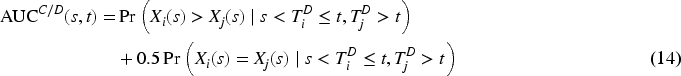


The cumulative/dynamic AUC at time
Estimates for the cumulative/dynamic AUC can be obtained by replacing transition probabilities and hazards by their estimated counterparts as follows:


To study the discrimination performance of an interval-censored binary disease marker on survival a simulation study was conducted. Incident/dynamic and cumulative/dynamic AUC were computed for the different estimation procedures presented in Section 2: the Cox model with time-dependent disease marker, which ignores interval-censoring, and the illness-death model with piecewise-constant, Weibull or M-spline transition hazards. For the piecewise-constant model, the four change points
Data generation and methods
Data were generated from Weibull transition hazards with a common shape parameter
Draw Decide which transition If If If the individual entered the disease state, draw Censor the true death time according to the desired censoring scheme: Administrative censoring: the survival time is Uniform random censoring: draw the censoring time Let Return the time-to-death outcome


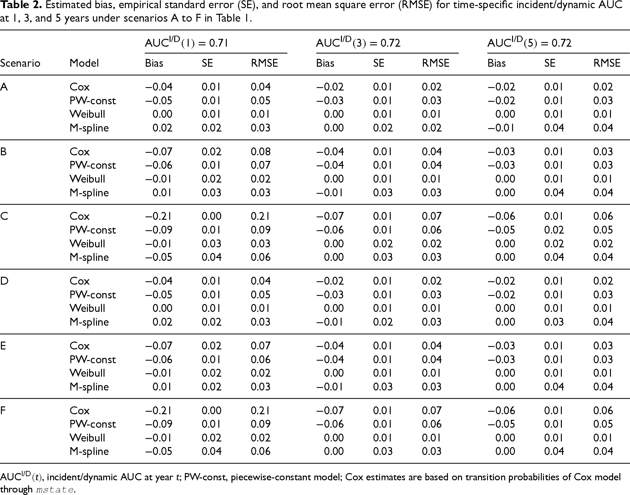
Table 1 summarizes the 18 scenarios (A–R) generated using shape parameter
Simulated scenarios.
Simulated scenarios.
The true incident/dynamic and cumulative/dynamic AUC values over time were determined using equations (9) and (15), where the terms
Estimated models
HRs for disease (yes vs. no) were estimated for the piecewise-constant and the Cox model. Average values over
The M-spline model did not converge for many simulated data sets, with the frequency of invalid estimations (Supplemental Table C.2) increasing as sample size decreased. These difficulties are partly attributable to the decision not to implement automatic smoothing parameter selection due to potential numerical instability in simulations and to avoid manual tuning to ensure comparability across datasets. These invalid estimates prevented the estimation of the incident/dynamic and cumulative/dynamic AUCs. Therefore, the results for the M-spline model shown in Sections 4.2.2 and 4.2.3 are only based on the obtained valid estimates.
Since average AUC estimates were nearly identical between scenarios where only the sample size differed, only results for scenarios A to F with
Incident/dynamic AUC
For each model and scenarios A to F, Table 2 shows the bias, empirical SE, and RMSE for estimates of the incident/dynamic AUC at years 1, 3, and 5, which coincide with the times of follow-up visits for every scenario. The Weibull model outperformed the other models in each scenario. This is not surprising since the data were generated according to Weibull distributions. The M-spline model consistently had the largest empirical standard error as well as the second smallest bias overall. The piecewise-constant model was slightly less biased than the Cox model for scenarios with 6 and 12 months between follow-up visits (scenarios B, C, E, and F). For the scenarios with 3 months in between follow-up visits, the Cox model outperformed the piecewise-constant model (scenarios A and D) in terms of bias. The follow-up schemes with larger intervals resulted in larger bias of the incident/dynamic AUC estimates, particularly for the Cox model. Although the censoring scheme impacted the valid estimates of the M-spline model (Supplemental Table C.2), it did not have a major effect on the AUC estimates for the Cox, piecewise-constant, and Weibull models.
Estimated bias, empirical standard error (SE), and root mean square error (RMSE) for time-specific incident/dynamic AUC at 1, 3, and 5 years under scenarios A to F in Table 1.
Estimated bias, empirical standard error (SE), and root mean square error (RMSE) for time-specific incident/dynamic AUC at 1, 3, and 5 years under scenarios A to F in Table 1.
Figure 2 shows the estimated incident/dynamic AUC over years, that is,
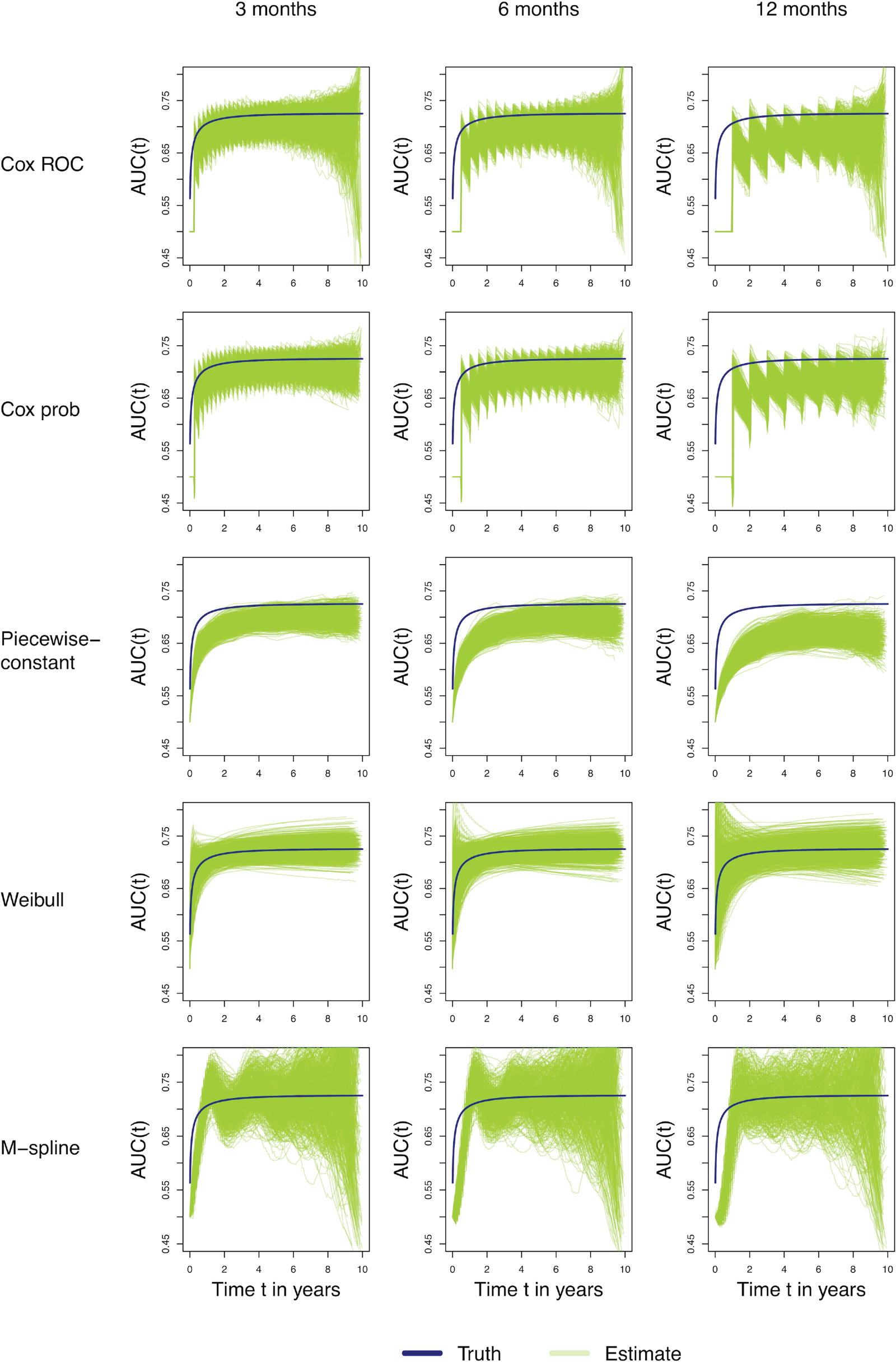
Estimated time-specific incident/dynamic AUC for scenario A (3 months; left panels), B (6 months; middle panels), and C (12 months; right panels) using different models (Cox, PW-const, Weibull, and M-spline). The x-axis represents time
Table 3 shows the bias, empirical SE, and RMSE for estimates of the incident/dynamic AUC at years 1, 3, and 5 for the four models in scenarios A to F. The piecewise-constant model showed the worst performance and underestimated the true AUC. The Weibull model, M-spline, and the Cox model provided good results. The follow-up scheme with larger intervals resulted in consistently more biased estimates for the piecewise-constant model. The Cox, Weibull and M-spline model based estimates were of limited bias for the different follow-up schemes. Again, although the censoring scheme impacted the valid estimates of the M-spline model (Supplemental Table C.2), it did not have a large effect on the AUC estimates for the other models.
Estimated bias, empirical standard error (SE), and root mean square error (RMSE) for time-specific cumulative/dynamic AUC for prediction time 1, 3, and 5 years and prediction window of 5 years under scenarios A to F in Table 1.
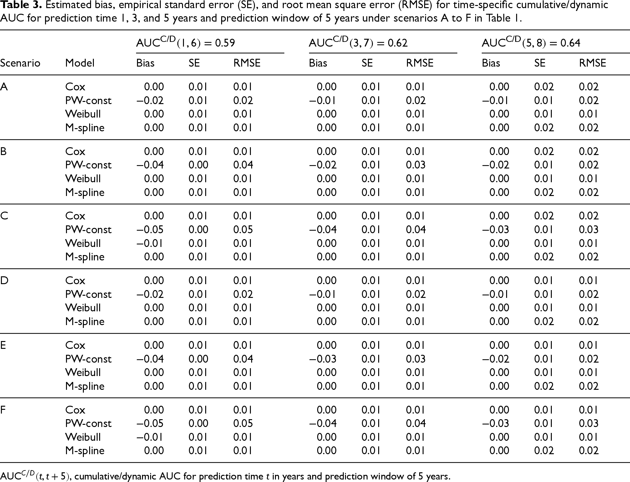
Estimated bias, empirical standard error (SE), and root mean square error (RMSE) for time-specific cumulative/dynamic AUC for prediction time 1, 3, and 5 years and prediction window of 5 years under scenarios A to F in Table 1.
Figure 3 shows the estimated cumulative/dynamic AUC over years with a prediction window of 5 years, that is,
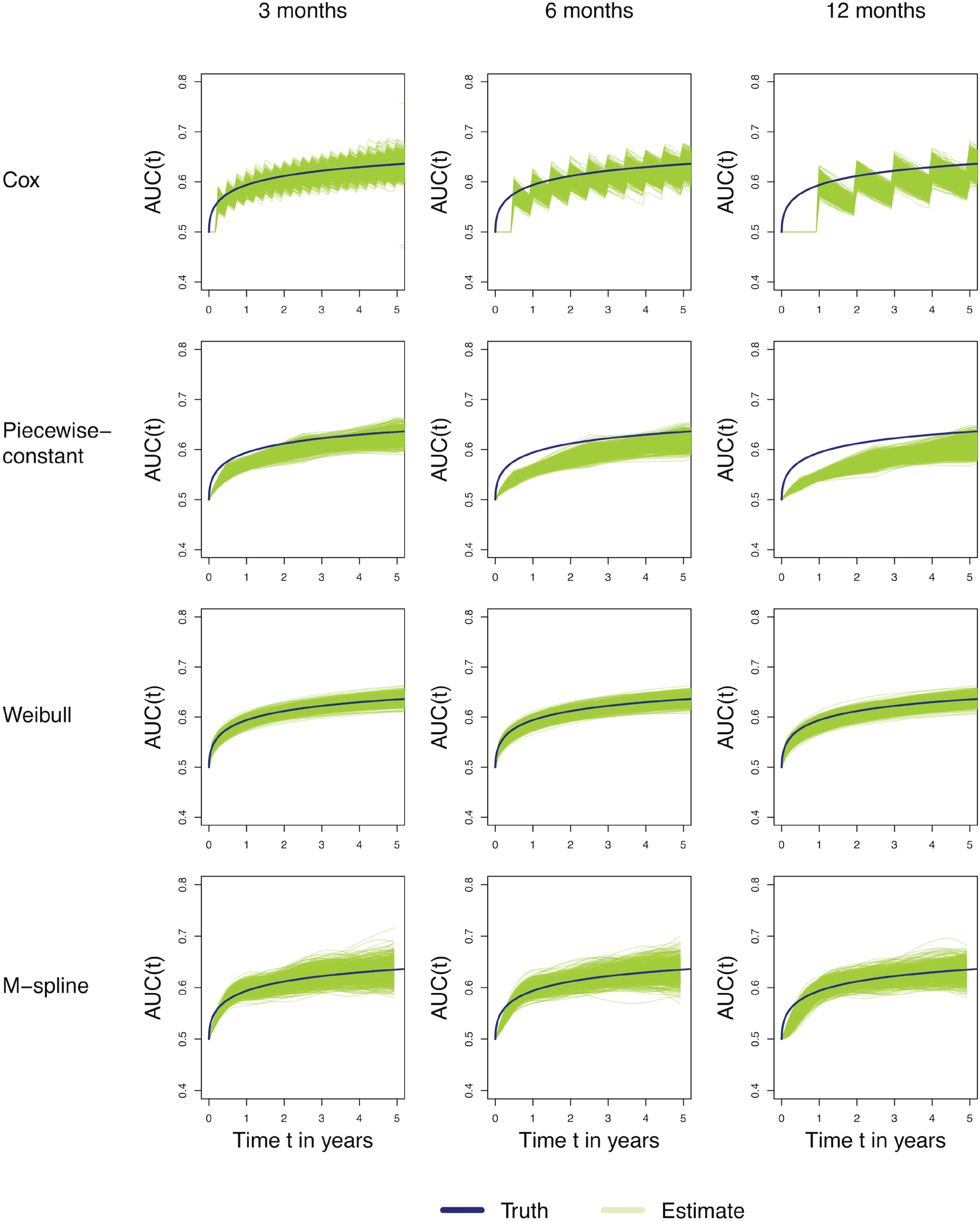
Estimated time-specific cumulative/dynamic AUC for scenarios A (3 months; left panels), B (6 months; middle panels), and C (12 months; right panels) using different models (Cox, PW-const, Weibull, and M-spline). The x-axis represents the prediction time
Soft tissue sarcoma data
The data analyzed in this section was used for the development of a dynamic prediction model for patients with high-grade soft tissue sarcoma. 29 The data set contains follow-up information of 2232 patients treated surgically with curative intent. Median follow-up time was 6.42 years. After surgery disease progression can be described by several adverse events: a patient may develop a local recurrence and/or develop distant metastases (DM) and/or die. The analysis discussed in this section focuses on the effect of DM on death. In total 1034 patients died and 715 patients first developed DM (see Figure 4).

Soft tissue sarcoma illness-death model (
After surgery, a common scheme of follow-up visits for DM screening involves the patient being seen every 3 months during the first 3 years, then every 6 months until the fifth year, and once a year thereafter. 30 The data did not contain information about exact follow-up times and an approximation of disease screening times was applied to the data. For a patient who was diagnosed with DM during follow-up, the time of DM specified in the data was interpreted as the first positive screening for DM. Since the time of the last negative screening was unknown an approximate time of last screening was assumed: if DM was diagnosed within the first 3 years of follow-up, between 3 and 5 years, or after 5 years the previous screening was assumed to have taken place either 3, 6, or 12 months prior to DM diagnosis. A patient who was never diagnosed with DM was assumed to have been screened according to the common follow-up scheme described above.
The four models presented in Section 2 were estimated for the soft tissue sarcoma data, and time-specific incident/dynamic and cumulative/dynamic AUCs introduced in Sections 3.1 and 3.2, respectively, were computed.
The HRs estimated by the Cox model and the piecewise-constant model were equal to 11.71 (95% CI = [10.31; 13.29]) and 11.28 (95% CI = [9.82; 12.96]), respectively. For the M-spline model,
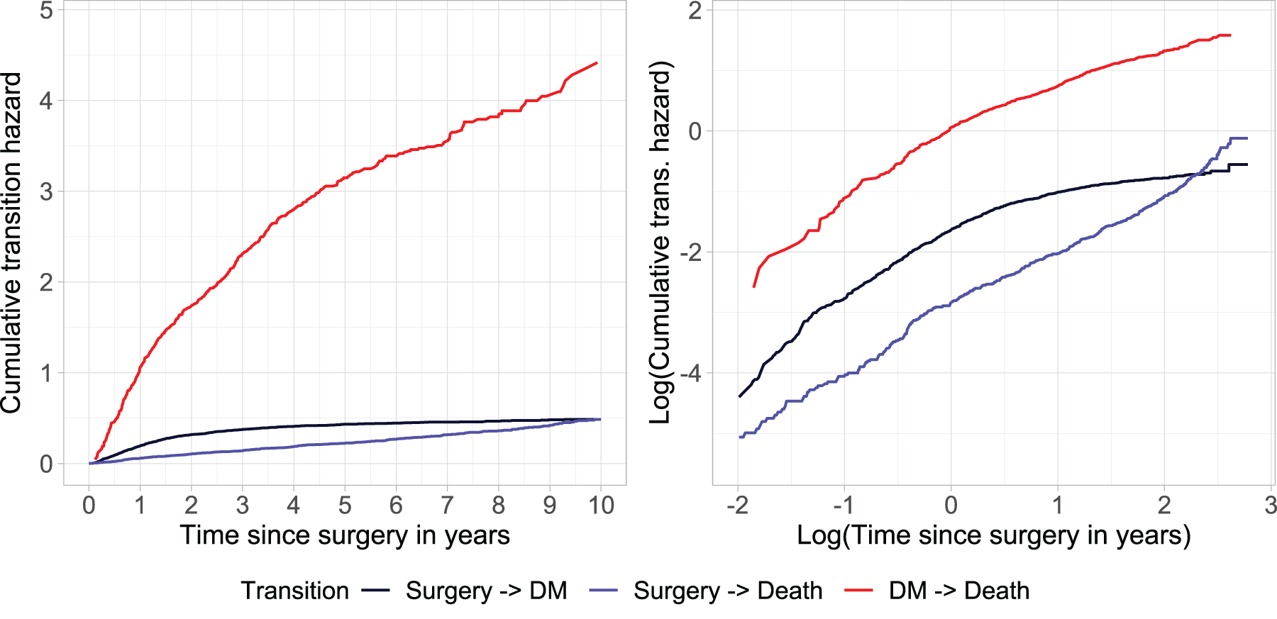
Left panel: Cumulative transition hazards. Right panel: plot of logarithm of cumulative transition hazards versus logarithm of time (in years) to empirically check the fit of the Weibull distribution.
Figure 6 shows the AUCs over time for the different models (left panel: incident/dynamic; right panel: cumulative/dynamic), with time-specific values at years

Time-specific AUC of the binary time-dependent marker
Estimated discrimination performance of the binary time-dependent marker
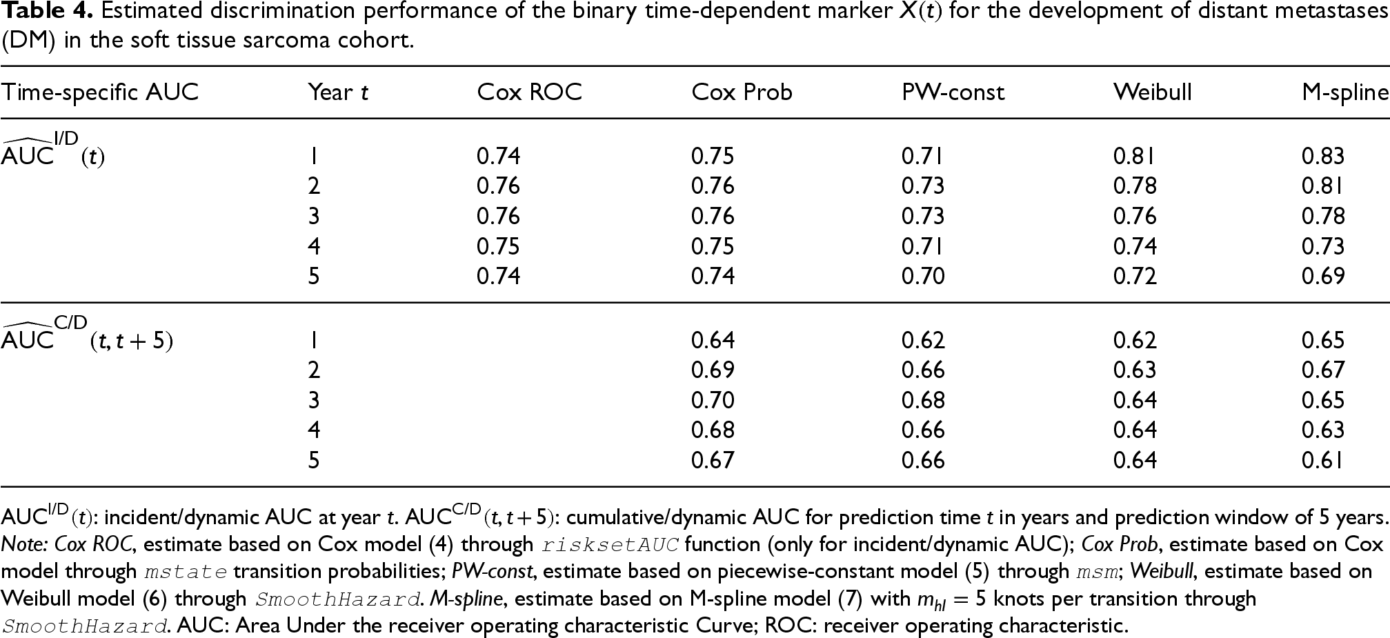
Note: Cox ROC, estimate based on Cox model (4) through
The illness-death model is frequently applied to clinical data to describe disease progression. A patient enters the model disease free, may then experience disease and die. In clinical practice, however, the time of disease onset cannot often be observed exactly. The information is interval-censored or not observed due to death or censoring. This can lead to bias in the estimation of disease incidence and regression coefficients.4,6,8,11
This article studied the discrimination performance of a binary time-dependent disease marker in the context of the illness-death model for interval-censored data. A simulation study with several data scenarios was conducted to study four different models: the Cox model with disease as time-dependent marker, the piecewise-constant model implemented in the
The simulation study showed that the HRs from the piecewise-constant model were less biased than those of the Cox model. The number of patients per data set (400 vs. 1000 vs. 2000) did not have a large effect on the estimates of the HR, AUC estimates in incident/dynamic and cumulative/dynamic definition, except for the M-spline model which converged more reliably with large data sets (see Supplemental Material C). The type of censoring scheme did mostly influence AUC estimates based on the Cox model and M-spline model, since hazard estimates are non-parametric and therefore more sensitive at later time points at which fewer events are observed. The Weibull model demonstrated the best performance; however, it had an inherent advantage, as the simulated data followed a Weibull distribution. In practice, a Weibull distribution may not be a good fit to the data, as shown in the soft tissue sarcoma application. The M-spline model showed a good performance when estimating the incident/dynamic and cumulative/dynamic AUC, however, was not always able to converge and provide AUC estimates. AUC estimates based on the piecewise-constant model in the incident/dynamic definition had less bias than those based on the Cox model for scenarios with large spacing between follow-up visits and in the cumulative/dynamic definition they had the largest bias of all methods. The spacing of follow-up visits at which the disease state was observed did have a large effect on estimates of the incident/dynamic AUC, particularly for the Cox model. The cumulative/dynamic AUC depends solely on transition probabilities, whereas the incident/dynamic AUC also depends on the underlying transition hazards. Consequently, discrimination measured by the cumulative/dynamic AUC is largely insensitive to differences in baseline hazard specification. This explains why the considered methods do not generally outperform the Cox-based approach for cumulative/dynamic AUC, particularly at follow-up visit times when the Cox model exhibits lower bias.
In practice, depending on how reasonable the assumption of Weibull distributed transition hazards is, one could choose to estimate the AUCs based on the Weibull or M-spline model. However, it is crucial to consider that convergence of M-spline models can be affected by smoothing parameter selection or numerical instability. Automatic smoothing parameter selection via cross-validation, while generally effective, can be computationally intensive, and manual tuning is often challenging in complex datasets and not always feasible in simulation studies. In our application, rescaling the time variable enabled convergence under automatic smoothing parameter selection, highlighting the importance of careful numerical considerations in spline-based modeling. Specifically, extreme values or a wide range of time points can lead to poorly scaled basis functions and penalty terms, complicating optimization and potentially preventing convergence.
The choice between incident/dynamic and cumulative/dynamic discrimination metrics depends on the specific perspective of interest, yet both are scientifically relevant. Incident/dynamic AUC is most appropriate when the focus is on the marker’s ability to identify, at a given time, which individuals who are still at risk are most likely to experience death shortly thereafter. This can be particularly informative for time-specific decision-making, such as screening or monitoring. In contrast, cumulative/dynamic AUC evaluates the marker’s ability to discriminate which individuals who are still at risk at a given time are most likely to experience death before a given time horizon, thereby capturing its long-term prognostic capacity. Since clinical and research objectives may require either short-term or cumulative assessments, considering both approaches provides a more comprehensive evaluation of marker performance.
A limitation of multi-state models, such as the illness-death model, is that small sample sizes (e.g. 100 or 200 subjects) often lead to unreliable estimates, even when event times are exactly observed, due to the complexity of modelling multiple transitions and the potential sparsity of events. This issue is further amplified in the presence of interval censoring. Consequently, caution is warranted when applying the proposed methods in such settings. Moreover, it was implicitly assumed that the visiting process did not depend on the state (diseased and non-diseased). In clinical practice, however, this may not always be a reasonable assumption. Patients may visit the clinic earlier if they have complaints that are related to being in the diseased state. The effect of an informative visiting process could be a subject of future research.
The performed simulations examined the effect of an interval-censored binary disease marker. Future research could explore the discriminatory performance of an interval-censored, time-dependent covariate with more than two possible values, that is, a subject that can transition between multiple disease states. This would require estimation methods for general interval-censored multi-state models, which have been developed only in recent years.31–33 Another topic of future research could be to investigate a different definition of the incident/dynamic AUC. At time
This study highlights the importance of considering the interval-censored nature of disease data in both parameter estimation and the evaluation of discrimination performance for disease development. This consideration is crucial as prediction models are nowadays increasingly important in clinical practice to provide personalized patient care.
Supplemental Material
sj-pdf-1-smm-10.1177_09622802251412855 - Supplemental material for Discrimination performance in illness-death models with interval-censored disease data
Supplemental material, sj-pdf-1-smm-10.1177_09622802251412855 for Discrimination performance in illness-death models with interval-censored disease data by Marta Spreafico, Anja J Rueten-Budde, Hein Putter and Marta Fiocco in Statistical Methods in Medical Research
Footnotes
Acknowledgements
The simulation study was performed using the compute resources from the Academic Leiden Interdisciplinary Cluster Environment (ALICE) provided by Leiden University. Prof. Dr Michiel van de Sande and the PERsonalized SARcoma Care (PERSARC) study group are gratefully acknowledged for making the soft tissue sarcoma data set available. PERSARC study group: Lee M Jeys, Minna K Laitinen, Rob Pollock, Will Aston, Jos A van der Hage, Sander Dijkstra, Peter C Ferguson, Anthony M Griffin, Julie J Willeumier, Jay S Wunder, Emelie Styring, Florian Posch, Olga Zaikova, Katja Maretty-Kongstad, Johnny Keller, Andreas Leithner, Maria A Smolle, and Rick L Haas.
Funding
The authors disclosed receipt of the following financial support for the research, authorship, and/or publication of this article: AJR-B was supported by the KWF Kankerbestrijding grant UL2015-8028. MS was supported by the KWF Kankerbestrijding grant 2023-3 DEV/15461. The funding sources had no involvement in study design, in the collection, analysis and interpretation of the data, in writing of the report, and in the decision to submit the article for publication.
Declaration of conflicting interests
The authors declared no potential conflicts of interest with respect to the research, authorship, and/or publication of this article.
Data availability statement
Supplemental material
Supplemental materials for this article are available online.