Impact of COVID-19 on the Income of Entrepreneurs Who Borrowed from SHG

Abstract

The COVID-19 pandemic has shaken the world. After liberalization in 1991, microfinance became a panacea for poor people without collateral and information asymmetry. The higher cost of microfinance and debt traps highlighted the need for the state to intervene in resource redistribution. In addition, national lockdowns and COVID-19 restrictions have made it difficult for emerging economies like India to achieve this sustainable development goal. The Reserve Bank of India introduced self-help group (SHG) bank linkage to ensure the financial inclusion of the poor. The difference-in-difference method examined how SHGs affect entrepreneur households’ income. CMIE Consumer Pyramid dx data were used for analysis. The data establish that SHGs have increased the income of the households, and demographic factors such as education, income level and gender also impact the financial inclusion of the poor.

Keywords

Self-help group microfinance COVID-19 U.N. sustainable development goals

Introduction

Financial inclusion as a sustainable development goal implies access to and usage of financial services (Demirguc-Kunt & Levine, 2008). COVID-19 posed severe challenges to attaining the goal of inclusive development (Tchamyou, 2018). According to CMIE Consumer Pyramid data, the COVID-19 outbreak resulted in substantial decreases in economic activity in India and led to the financial exclusion of the poor. There is a dearth of the theory of personal finance and microfinancing for small entrepreneurs that enumerates what factors affect the financial choices of households (Lusardi & Tufano, 2015). COVID-19 impacted the attainment of the goal of financial inclusion differently in different parts of the globe, depending on the scope and pace of development (Asongu & Nting, 2020). Emerging economies such as Vietnam, China and India have developed policies for financial inclusion and funding entrepreneurs during COVID-19. This includes subsidized loans of 3 trillion USD to small entrepreneurs in India. The European Commission released a fund of 8 billion Euros in Europe to aid small entrepreneurs. Despite all efforts, the pandemic highlighted various gaps in development policies towards financial inclusion in emerging economies. India witnessed different demand and supply challenges to attaining inclusive growth during COVID-19, as 82% of the small entrepreneurs and 84% of the households were affected by the pandemic with an income loss. Access to formal finance without collateral became a challenge on the supply side, as most formal financial institutions, including MFIs, found it financially unviable to finance the poor. On the demand side, various factors such as education, type of occupation and gender jeopardized the attainment of financial inclusion goals. During COVID-19, the dependence of the poor on informal sources of finance increased dramatically. Due to a lack of collateral and information asymmetry, SHGs emerged as a panacea to the financial exclusion of the poor in India. This study aims to discuss the impact of various factors on households’ personal financing decisions from a policy perspective during COVID-19.

Literature Review

Emerging economies suffer poverty, which is typically associated with market failure. 60% of the impoverished live in lower middle income countries. Thus, the market-based approach fails in lower middle income countries (Banerjee & Jackson, 2017). Donations and subsidies managed poverty until 1990. Since 1991 in a liberalized world, governments worldwide have accepted the paradigm of sustainable development based on self-reliance (Roy, 2011). Informal finance drives small business growth in India (Kislat, 2015). Microentrepreneurs prefer informal debts due to the requirement of loans at a higher frequency and lack of collateral. Moreover, due to information asymmetry, financial institutions do not have information about the creditworthiness of the poor. This is one of the significant challenges for poor households and small entrepreneurs in India (Sinha et al., 2012). The personal financing mix of the households depends on two kinds of factors: (a) individual factors and (b) contextual factors (Nguyen & Canh, 2021). However, unlike corporate finance, no theory sheds light on the financing decisions of households or small businesses (Lusardi & Tufano, 2015). This study will address the research gap in terms of the lack of a theory of personal finance that addresses the trade-off between formal and informal finance in accessing external finance by poor households and entrepreneurs (Wu et al., 2017). For this purpose, we define personal finance for households as (a) informal finance, (b) formal finance and (c) microfinance. This study defines informal finance as finance from (a) shops and (b) relatives, and formal finance as credit from banks. Microfinance is defined as (a) microfinance institutions and (b) SHGs. The primary reason for the dependence of poor households on informal finance is financial exclusion (Hoff & Stiglitz, 1990). Financial inclusion is vital in promoting development and reducing poverty levels (Mader, 2018). India managed poverty using pro-poor, developmental and democratic participatory banking, democratic engagement, articulating the poor’s viewpoint and boosting entrepreneurship. The SHG linkage programme gives voice to the masses who own the labour and do not own the factor of production (Liegey & Nelson, 2020). This is akin to Marx’s idea of power within a group of people with common economic interests (Marx, 1996). Microfinance became the baton for female entrepreneurs supported by self-help organizations to overcome the epidemic’s doom, especially from a feminist stance (Armendariz & Morduch, 2010; Gopal & Malliasamy, 2022; Neely & Carmichael, 2021; Onuka, 2021; Pitt & Khandker, 1998). Microfinance in the form of SHGs allowed small entrepreneurs to get loans without physical collateral by utilizing social capital, trusts and relationships (King & Levine, 1993; Maclean, 2010; Morduch, 1999; Weber, 2004). There is no empirical study to measure the impact of COVID-19 and policy decisions on accessing microfinance through group lending. Thus, this research study aims to measure the impact of SHGs on the financial outcomes of community groups during COVID-19 (Desai & Joshi, 2014).

As per Hanning and Jansen (2010), financial inclusion allows financial stability, and the literature highlights that various factors impact financial inclusion. This study aims to measure the impact of multiple factors, such as gender, education, income and COVID-19, on financial inclusion and the personal financing mix of households in India. The research studies highlight the presence of gender disparity, and the issue of gender difference in accessing finance is a topic of immense debate. However, there is a lack of studies that discuss the impact of gender disparity on personal financing decisions during COVID-19. This provides an important insight for the policymakers, which states that special social intermediation initiatives must be designed to cater to the needs of women borrowers.

Earlier studies show that financial literacy programmes have made it easier for consumers to get credit. Poor people generally have inadequate knowledge about personal finance. Various supply and demand side factors impact financial inclusion. Demand side factors include the poor’s lack of financial literacy and financial knowledge (Nagayya & Rao, 2009). Our model shows that formal education boosts formal loan access (Brown et al., 2013), (Huston, 2010). Thus, this study explores the impact of formal education on people’s financial behaviour. The lack of formal education among the poor is a less researched area, due to which this study makes a relevant contribution to the literature.

This study aims to analyse the impact of COVID-19 on the personal financing choices of microentrepreneurs and households. It seeks to contribute to the literature on the theory of personal finance, which is not a researched area.

Research Problem

The goal of this study during COVID-19 is to see how microfinance in the form of SHG borrowings affects household economic well-being or average income. The CMIE Consumer Pyramid survey, collected from January 2019 to April 2021, provided the data for this study. In this study, the difference-in-difference (DiD) design is used to investigate the influence of the intervention on the sample’s economic well-being.

RQ1: What is the impact of COVID-19 on the average household income of those who borrowed money through SHGs?

RQ2: What is the impact of the regional divide during COVID-19 & demographic factors on the personal financing decision of the households?

Methodology

This study analyses how microfinance through SHGs affects borrowers’ financial stability during COVID-19. We used the CMIE Consumption Pyramids data for analysis. CMIE provides data in the form of waves of 4 months each. We have taken three years, and hence there are nine periods. We took data for nine different waves, that is, January–April 2019, May–August 2019, September–December 2019, January–April 2020, May–August 2020, September–December 2020, January–April 2021, May–August 2021, September–December 2021. Data from March 2020 to December 2021 was utilized as the post-COVID period, and data from January 2019 to March 2020 was used as the pre-COVID period in this research.

The panel data used in these surveys represent the national, rural and urban levels. For analysis, we chose 2,361 households at random from the complete survey. We initially employed parallel graph analysis to compensate for time-invariant oscillations in the data. The DiD methodology can regulate individual fixed effects. We employed the DiD regression using panel data to analyse the causal influence of SHGs on the income of households. DiD is justified because randomization on an individual level is impossible. Since the objective of the study is to determine the impact of social interventions such as SHGs on poor members of society. We also employed the mixed regression method to estimate the impact of SHG borrowing on average income to provide for the time-bound inconsistencies.

Data Analysis

Description of Data

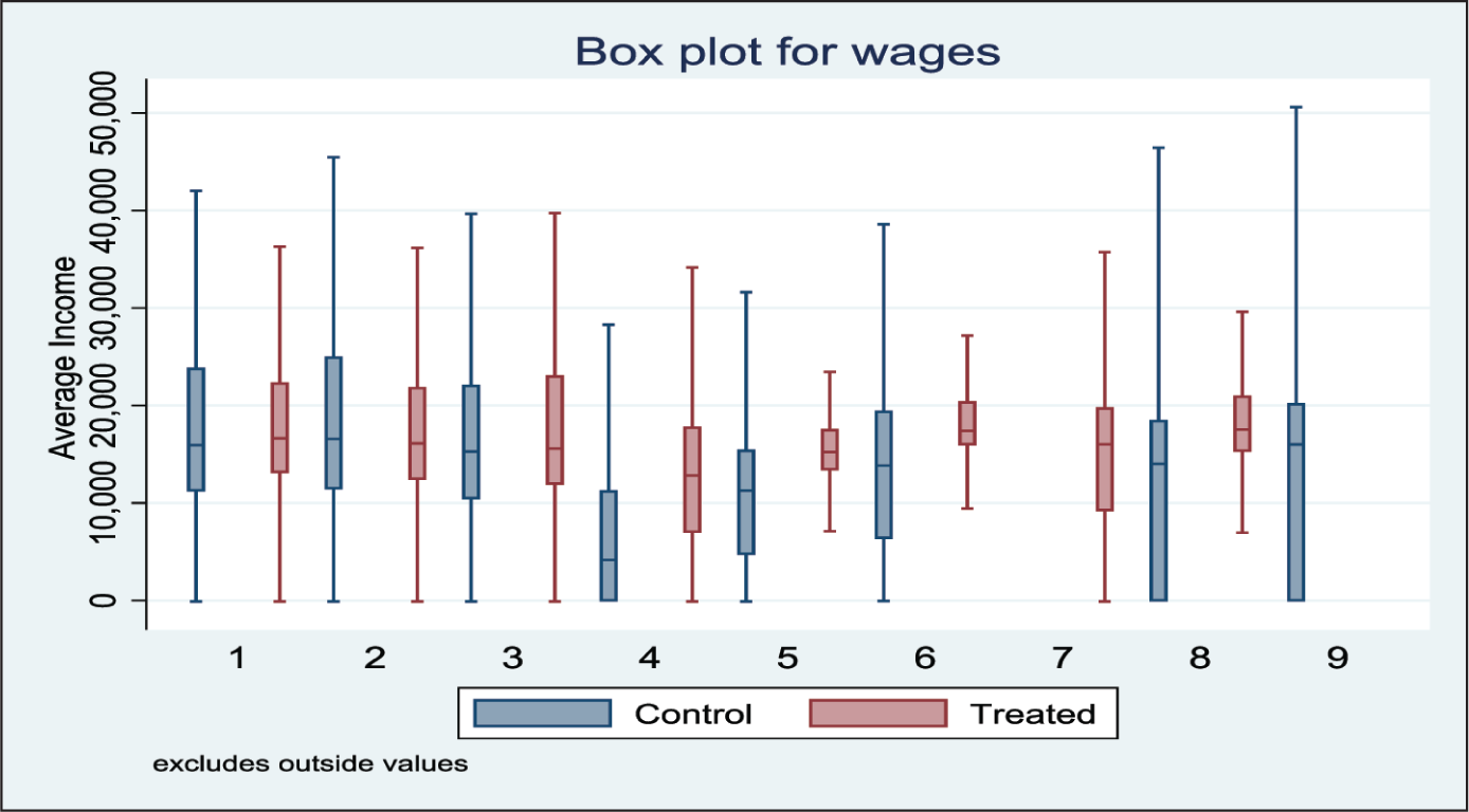
The box plot in Figure 1 above describes the data for nine periods from January 2019 to December 2021. The control group is comprised of the households that did not borrow from the SHG and treated are those that borrowed from the SHGs. Period 5 is the period of setting in of the COVID. And the interquartile range of the average income of people who borrowed during the pandemic, that is, fifth and sixth cycles, shows a significant decline. In contrast, the interquartile range of the control group increased tremendously. However, the boxes of the treated group during the pandemic remained above the control group in all the periods about the treated group, which implies that SHG borrowing reaped benefits for the households. There was an overall increase in the income of the households that borrowed from the SHGs during COVID-19.

Figure 1.

Box Plots for the SHG in Rural and Urban Areas During Pre-COVID (Control) and Post-COVID.

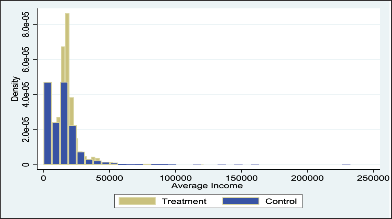
Distribution of the sample data between the pre-treatment (COVID) and post-treatment (COVID) period is given in Figure 2.

The treatment and control groups’ distributions overlap for the lower income levels. This is expected; however, the average income increases with the treatment effect, that is, the implementation of the SHG programme. Thus, the treatment households might have had a higher average income in the pre-COVID period, as shown in Figure 2.

Figure 2.

Distribution of Average Income of Members Who Took SHG Loan in the Pre-COVID Period.

Figure 3 compares the same distribution in the follow-up years 2020 and 2021. We observe that the treatment households are doing better than the control groups.

Figure 3.

Distribution of the Average Income of Members Who Took SHG Loan in the Post-COVID Period.

Next, we tested the baseline balance of the covariates used in the DiD estimation. During the pre-COVID and post-COVID periods, there were significant differences between the treatment group and the control group based on the period of aggregation that is COVID-19 and, accordingly, beneficiaries of the schemes by the state within the ambit of SHG loan borrowings. Our covariates are mainly education, gender of household, number of members in the household and region.

Table 1 shows that overall, the average income of the households that borrowed from the SHGs is significantly higher than the control groups. Expenditure levels, education, gender and the number of members in a household have a positive and significant impact on the income of households.

Table 1.

Difference-in-Difference Estimation Results.

	Mean Control	Mean Treated	Difference	T Statistics	P(ϰ)
Average income	1,50,000	1,70,000	2,301.75	9.17	0.000***
Expenses	8,387.18	9,628.32	1,241.14	11.98	0.000***
Education	3.142	3.549	0.408	11.62	0.000***
Gender	0.521	0.381	–0.141	13.69	0.000***
Number of members	2.711	3.302	0.591	23.48	0.000***
Region	0.303	0.385	0.082	8.32	0.000***

Notes: *P < .1, **P < .05, ***p < .01.

Average Treatment Effect

In both the pre-treatment and post-treatment periods, the average treatment effect estimator is the difference between the control and treatment groups. Calculating the pre-treatment difference between the treated and control groups, as well as the post-treatment difference between the treated and control groups, is necessary to determine the average treatment effect (Albouy, 2012).

If we take a simple model in which the difference is calculated in the outcome before and after the treatment, the results will be biased:

δ_{1} = {\bar{Y}}_{t 1} - {\bar{Y}}_{t 0} .

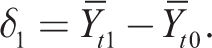
This means that as long as the time trend in the outcome Y_i exists, the estimator will be biased, and the time trend will be confounded as part of the treatment effect. In many circumstances, the estimator is calculated by comparing the average difference in result Y_i post-treatment between the treatment and control groups without considering the pre-treatment outcomes. If the assumption of a shared trend between the treatment and control groups is violated, one of the fundamental issues with the DiD estimator arises. Otherwise, the estimation will be skewed if the treatment and control groups have the same trend. We used the parallel trend method to resolve the confoundedness in the case of a data panel.

The estimator is based on comparing the average difference in outcome Y_i post-treatment between the treatment and the control groups, ignoring the pre-treatment outcomes.

Δ_{2} = {\bar{Y}}_{t 1} - {\bar{Y}}_{c 1} .

Figure 4.

Difference-in-Difference Graph for the Treated and Control Groups.

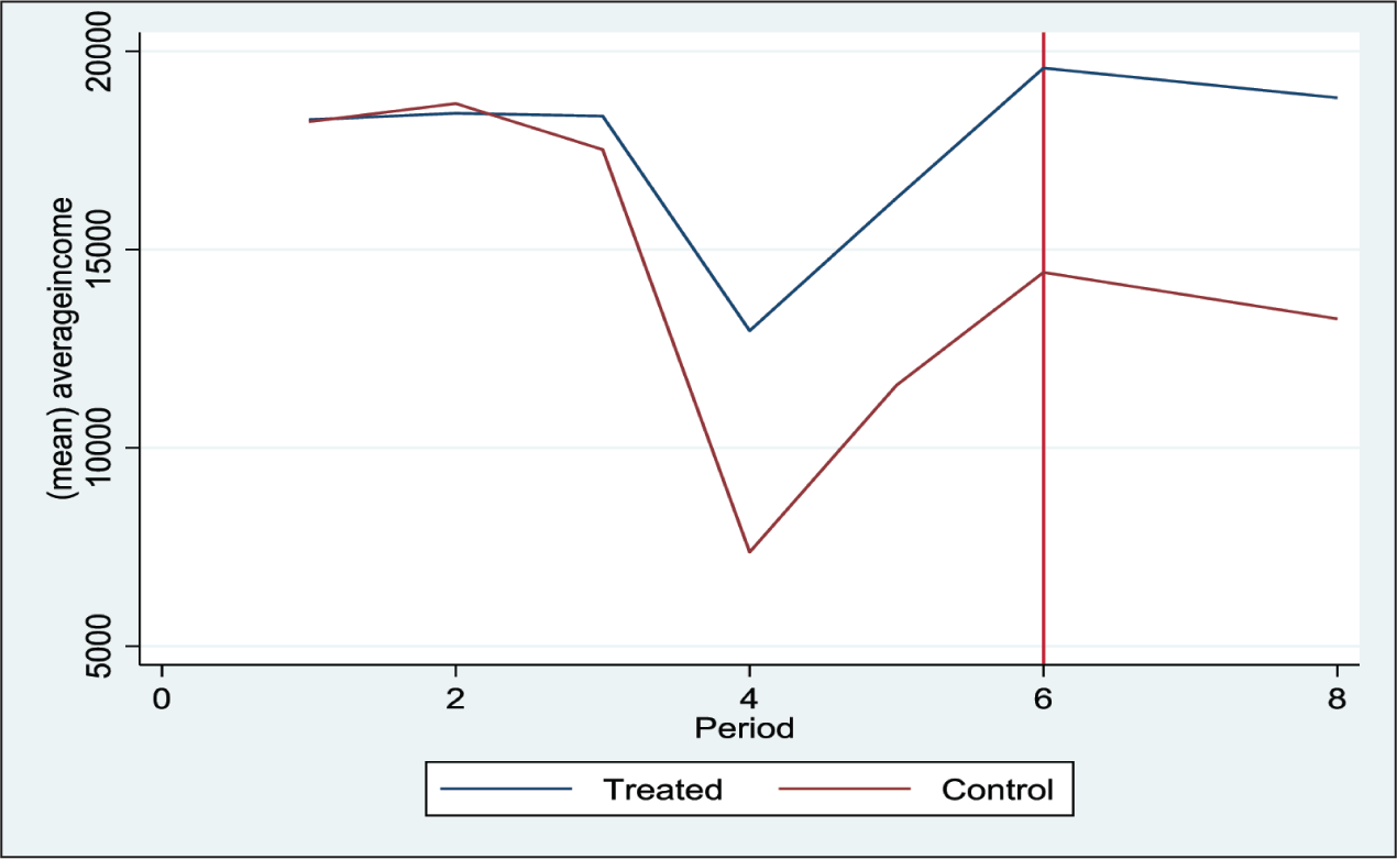
Figure 4 exhibits the presence of parallel trend in the data that authenticates the use of difference in difference. The actual treatment effect will be masked by the permanent differences in the treatment and control groups before treatment. This refers to the model’s fixed individual effects. According to the model’s analysis, the fixed effects are appropriately modified when calculating the DiD effects in a panel that consists of the same individuals. To estimate the average treatment effect using the DiD method, the regression equation has been specified as follows:

Y_{i} = α + β T_{i} + γ t_{i} + δ (T_{i} • t_{i}) + ε_{i} .

In this model, T refers to the treatment group, and β relates to the group-specific effect that accounts for the average permanent differences between the control and treatment. Γ refers to the time trend common to both control and treatment groups. Δ refers to the actual effect of the treatment.

The Difference-in-Difference for SHG Borrowing

To estimate the average treatment effects using the DiD method. The results of the DiD using t-test calculations are given in Table 2.

Table 2.

Baseline Difference in Covariates and Outcome of Interest Between Treatment and Control Groups in the Pre-COVID and Post-COVID Periods.

Variable	Mean Pre-COVID	Mean Post-COVID	Difference	T Statistics	Pr. (T > t)
Income	14,497.51	17,227.17	2,301.37	9.17	0.000***
Expenses	9,941.14	8,327.61	1,241,47	8.32	0.000***
Education	3.142	3.549	0.082	8.32	0.000***
Gender	0.521	0.381	–0.141	13.69	0.000***
No. of members	2.711	3.302	0.591	11.98	0.0000***
Region	0.303	0.385	0.408	11.62	0.000***

Note: ***p<0.01.

As per Table 2, in the initial t-test, it was apparent that the difference between the control group and the treatment group was significantly based on income, expenses, education, gender, number of members in the family and rural region. Table 2 shows that overall, the income of the rural households in our sample increased by ₹2,301.37 during COVID-19.

Matching

In this study, in Table 3, the treatment and control groups are matched using the propensity score kernel matching. A total of 21,249 households have been identified for analysis. Of total, 11,184 households are in the control group, and 10,065 groups are in the treated group. There were 9,444 households studied during the pre-COVID-19 and 11,805 households surveyed during the after-COVID-19 period. Table 4 shows that the key covariates are highly balanced at the baseline even though the differences between the treatment and the control groups are significantly different from 0 based on expenses, education, gender and the number of members.

Table 3.

Treatment and Control Groups.

	Before	After	Total
Control	5,413	5,771	11,184
Treated	4,031	6,034	10,065
	9,444	11,805

The Difference-in-Difference Estimation Results for Average Income as a Function of Covariates

Table 4 calculates the impact of SHG borrowing on household income, using the control and treatment groups as proxies for SHG borrowing. Based on expenditure, gender of the household (where gender represents the masculine gender of the household), number of members in the household and rural region, the difference in income of households with SHG borrowing is significant.

Table 4.

Impact of SHG Borrowing on Income.

	Coefficient	Std. Error	T Statistics	P Statistics
Expenses	1.556	0.022	69.25	0.000***
Education	1110.84	79.12	14.04	0.000***
Gender	1039.21	186.20	5.58	0.000***
Number of members	–516.16	83.57	–6.17	0.000***
Region	2116.042	198.045	10.68	0.0000***

Note: ***p<0.01.

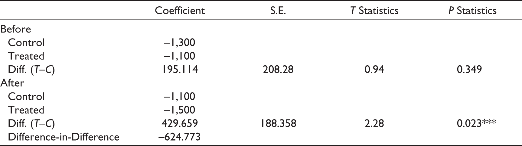
From the analysis of the results, the difference in income between the control and treatment groups after the COVID-19 period is highly relevant. After the COVID-19 period, the difference between the income of the control and treatment groups was ₹429.65, which is significant. This DiD analysis shows a substantial difference between the treated and the control groups. Table 5 shows the significant difference between the post-COVID-19 and pre-COVID-19 periods.

Table 5.

Difference-in-Difference Based on COVID-19 for the Control and Treatment Groups.

	Coefficient	S.E.	T Statistics	P Statistics
Before
Control	–1,300
Treated	–1,100
Diff. (T–C)	195.114	208.28	0.94	0.349
After
Control	–1,100
Treated	–1,500
Diff. (T–C)	429.659	188.358	2.28	0.023***
Difference-in-Difference	–624.773

Note: ***p<0.01.

Mixed Regression Model

CMIE Consumer Pyramids dx data are nested data, so we intend to use the mixed effect regression method. Unlike the normal ordinary least squares, which aims to reduce the residual, mixed regression seeks to minimize the deviance. Deviance is a more generalized form of error; like a full maximum likelihood method, this method considers both random and fixed effects. This method allows the researcher to compare both the fixed effects and the random effects. The mixed effect regression model is an unconditional model of time as each individual’s average income over the period can be represented as a trajectory. A model facilitates multilevel analysis. At Level 1, the data points and time can vary within the individuals; on a higher level, the slopes and intercept at Level 2 vary between the individuals. The data are indexed by the time point and by a participant.

L e v e l 1 : Y_{i j} = β_{0 j} + β_{1 j} (x_{i j}) + ε_{i j}

L e v e l 2 : I n t e r c e p t s : β_{0 j} =_{} γ_{00} +_{} U_{0 j};_{} L e v e l 2 : S l o p e s_{} β_{1 j} =_{} γ_{10} + U_{1 j},

where γ represents the fixed and group effects, which can be interpreted as the average intercept or average slope across the participants. Random effects U are the individual deviations away from the group-level effects. The final fixed and random effect model is

y_{i j} = γ_{00} + U_{0 j} + γ_{10} (x_{i j}) + U_{1} j (x_{i j}) + \int_{i j} .

has defined fixed effects as variables for which all the levels are present, and the random effect are variables that are only samples of the larger population. In a quasi-experimental study, the fixed effects of the group are the classification of the treatment and control groups, and the random effect will be the sample from the larger population.

Results of the Mixed Effect Regression Model

In this article, the study discusses the mixed effect regression model. Interactions between the period and individual treatment level, that is, SHG, show the effects of the period and treatment on individual slopes. In this model, the households are nested in the treatment.

Fixed Effect Model

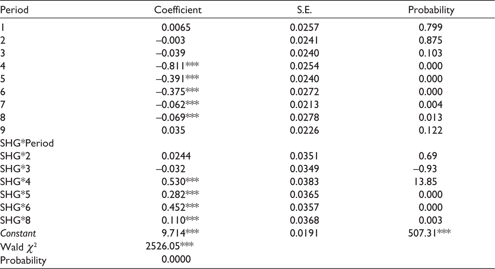
Table 6 depicts the fixed effects of SHG borrowing on the household’s average income. During the 4–8 periods, the income of the households decreased significantly. These were the periods of COVID-19. Further analysis of the SHG during the COVID-19 period depicts that the SHG has a significant impact on the income of the households during COVID-19, that is, the income of the households who have taken loans from the SHG increased significantly. Period 5 is the period of COVID-19. The income of the households that borrowed from the SHGs increased significantly during COVID-19, that is, during the periods 4, 5, 6 and 9.

Table 6.

Fixed Effects.

Period	Coefficient	S.E.	Probability
1	0.0065	0.0257	0.799
2	–0.003	0.0241	0.875
3	–0.039	0.0240	0.103
4	–0.811***	0.0254	0.000
5	–0.391***	0.0240	0.000
6	–0.375***	0.0272	0.000
7	–0.062***	0.0213	0.004
8	–0.069***	0.0278	0.013
9	0.035	0.0226	0.122
SHG*Period
SHG*2	0.0244	0.0351	0.69
SHG*3	–0.032	0.0349	–0.93
SHG*4	0.530***	0.0383	13.85
SHG*5	0.282***	0.0365	0.000
SHG*6	0.452***	0.0357	0.000
SHG*8	0.110***	0.0368	0.003
Constant	9.714***	0.0191	507.31***
Wald χ² Probability	2526.05*** 0.0000

Note: ***p<0.01.

Random Effect Model

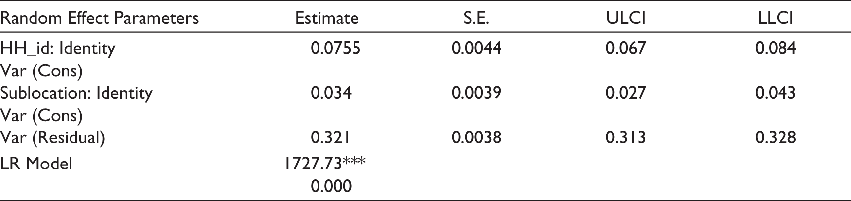
The random effects in Table 7 also depict that the results are highly significant.

Table 7.

Random Effects.

Random Effect Parameters	Estimate	S.E.	ULCI	LLCI
HH_id: Identity Var (Cons)	0.0755	0.0044	0.067	0.084
Sublocation: Identity Var (Cons)	0.034	0.0039	0.027	0.043
Var (Residual)	0.321	0.0038	0.313	0.328
LR Model	1727.73*** 0.000

Note: ***p<0.01.

Impact of the Regional Divide, COVID-19 and Poverty on the Propensity to Take a Formal Loan from Various Sources

To measure the causal impact of gender during COVID on the propensity to take a loan from different sources such as SHGs, banks, non-banking finance companies, microfinance institutions, shops and moneylenders, the article employs a DiD strategies. The period before COVID, April to May 2019, is taken as pre-COVID and the period from April to May 2021 is post-COVID.

\begin{array}{l} S o u r c e o f F i n a n c e_{i t} = β_{0} + β_{1} C O V I D . Re g i o n + β_{2} C O V I D + β_{3.} Re g i o n \\ + β_{4} I n c o m e S h o c k_{+} β_{5.} S c o r e + β_{6} . G e n d e r + X_{i} + M_{m} + ε_{i h d t}_{} \end{array}

Table 8 shows that during COVID-19, gender did not have any significant impact on borrowing from the SHG. Though overall the SHGs headed by males have a lower probability of borrowing from the SHGs. COVID-19 increased the propensity of borrowing from SHGs. Thus, during COVID-19 there was an increased propensity to borrow from SHGs.

Table 8.

Summary of Gender Impact on Borrowing from the SHG During COVID-19.

Variables	MODEL 1	MODEL 2
Variables	SHG	Bank
Male. COVID	–0.0958	–0.095
	(0.0657)	0.065
Male	–0.867***	–0.866
Male	(0.133)	0.133
COVID	0.0953*	0.095**
COVID	(0.0549)	0.054
Poverty score	–0.00157	–0.001
Poverty score	(0.00164)	0.001
Loginc	–0.0589*	–0.058**
Loginc	(0.0306)	0.030
Education	0.137	0.137
Education	(0.125)	0.124
Migration	0.223	0.222
Migration	(0.490)	0.490
Observations	18,156	18,156
Number of HH_id	9,078	9,078

Notes: *p<0.1, **p<0.05, ***p<0.01.

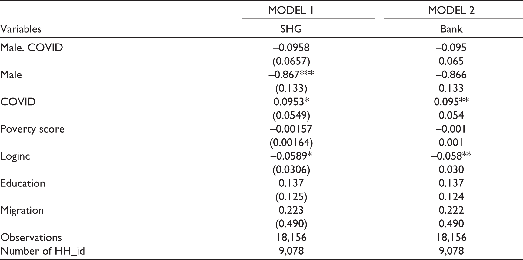
Difference-in-Difference (Male a Binary Variable, Depicts Households Headed by Males, COVID is a Binary Variable Where 1 is the Presence of COVID-19 and 0 is the Absence of COVID-19, Poverty Score Refers to Ownership of Assets—Calculated by Summation of Assets Owned. Education is a Binary Variable, 1 is an Educated Household, and 0 Uneducated Households, Migration is a Binary Variable, Where 1 is Family Migrated and 0 did not Migrate).

Table 9 analyses the impact of poverty and region on the propensity to borrow from various information sources such as non-banking finance corporations (NBFC), microfinance institutions (MFIs), banks, moneylenders and shops. Gender, income, education, poverty level, geography and occupation affect a household’s loan demand. Poor rural households borrow more from banks and moneylenders. Rural populations depend on informal sources like moneylenders because they can’t acquire formal loans without collateral, and various Government schemes like PMJDY promote lending to the poor by banks. Due to their superior financial capabilities and literacy, male-headed households are more likely to borrow from NBFCs than banks, MFIs, moneylenders and stores. Woman-headed households are more likely to borrow from moneylenders, shops and microfinance organizations due to inability, not lack of choices. Thus, financial literacy and education are needed to empower the disadvantaged through capacity building and financial inclusion. Social capital and government programmes helped the underprivileged get bank loans. However, poverty and illiteracy keep the poor dependent on moneylenders. Higher-income households borrow more from banks than moneylenders. Higher-income persons can borrow from formal institutions since they have better collateral. Higher-educated households borrow more from banks. Uneducated households borrow more from MFIs, moneylenders and shops. This financial behaviour of uneducated people is mostly due to a lack of financial education and awareness of financial services and goods. Literate persons comprehend financial service possibilities. They get state loans and subsidies.

Table 9.

Impact of Poverty and Region.

Variables	(1)	(2)	(3)	(4)	(5)
Variables	NBFC	Bank	MFI	Moneylender	Shops
Poverty. Rural	0.0361	0.0879**	0.339	0.301***	–0.0106
	(0.0846)	(0.0434)	(0.220)	(0.106)	(0.0295)
Poverty score	0.00134	–0.0464	–0.259	–0.292***	0.00240
	(0.0895)	(0.0463)	(0.230)	(0.111)	(0.0313)
Log income	0.00931	0.120***	–0.0451	–0.109**	–0.0126
	(0.0379)	(0.0317)	(0.103)	(0.0473)	(0.0133)
Migration	0.361	–0.325		0.00294	0.369*
	(0.915)	(0.355)		(0.779)	(0.219)
Male	0.217***	–0.426***	–0.457***	–0.584***	–0.0775***
	(0.0493)	(0.0284)	(0.155)	(0.0742)	(0.0181)
Education	–0.0705	0.120***	–0.418***	–0.481***	–0.424***
	(0.0620)	(0.0317)	(0.153)	(0.0729)	(0.0209)
Occupation	–0.0120	–0.0433*	0.226*	–0.325***	0.0718***
	(0.0445)	(0.0232)	(0.124)	(0.0571)	(0.0157)
Observations	9,520	36,010	1,370	6,616	78,738
Number of HH_id	4,760	18,005	685	3,308	39,369

Notes: *p<0.1, **p<0.05, ***p<0.01.

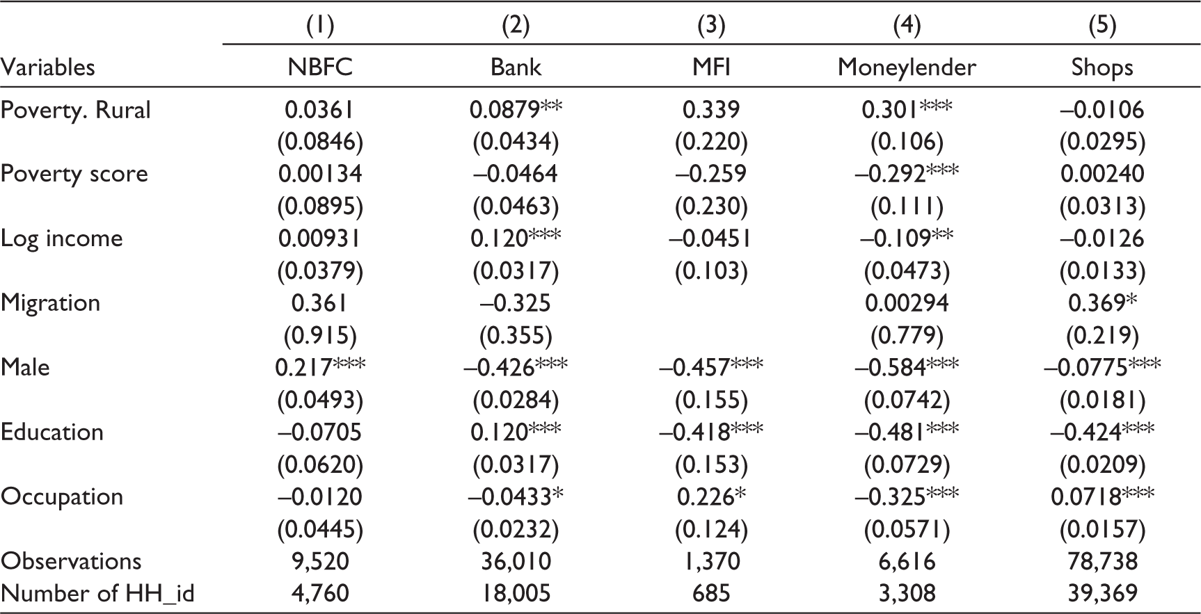
Standard errors in parentheses, *** p<0.01, ** p<0.05, * p<0.1. Poverty score refers to ownership of assets; Rural is a binary variable, where 1 is rural region; male is a binary variable for a household headed by males; Educated is a binary variable, 1 for educated households and occupation is a binary variable that refers to small and medium enterprises.

Discussion

From our analysis, we found evidence that during COVID-19, credit creation by SHGs increased and increased household income. This supports the finding of earlier studies that collaborative lending improves the income levels of households. The study finds evidence that factors such as gender, income and education impact credit generation through SHGs and banks. The study further demonstrates that higher-income individuals borrow less than low-income households. This conforms with earlier findings. They prefer savings to debt due to the higher risk of credit, which supports the pecking order theory.

Moreover, households headed by men borrow less from SHGs than women. This is because male-headed households have better livelihood opportunities and are more financially independent. Our study establishes that formal financial institutions tend to lend more to households headed by educated members. Moreover, educated households are better able to manage debt and repayment obligations, due to which the increase in education increases the propensity to borrow from the SHG banks and banks. Moreover, education minimizes the likelihood of borrowing from MFIs, moneylenders and stores. Female-headed households borrow more from moneylenders and shops than male-headed households. Females are less financially literate and have fewer financial services and credit options since they rely more on personal contacts and social networks, conformity with findings (Dang & Nguyen, 2021). Small entrepreneurs borrow more from MFIs than moneylenders, SHGs and banks. Small businesses prefer MFIs over banks because MFIs lend without collateral to improve entrepreneurial skills. Through micro-savings, micro-credit and micro-insurance, MFIs provide micro-entrepreneurs with the ‘silver bullet’ of financial inclusion. Our analysis confirms that microentrepreneurs access more loans from the shops as an informal channel due to the informational advantage and no need for collateral. Rural poor households prefer moneylenders. They lack financial awareness and collateral to access formal financial services. SHG bank linkage enables the poor to borrow by overcoming the information asymmetry. The Government of India has used MFI- and bank-financed initiatives for community groups and micro-borrowers to reduce financial exclusion, recognizing the social significance and acceptability of informal and semi-formal sources by low-income groups (Roodman & Morduch, 2014). The SHG bank linkage initiative improved bank credit for disadvantaged rural households.

Future Research

The impact of microfinance on rural income is highly debated. Capitalists believe that microfinance hurts the public’s finances. According to Marxists, microfinance improves the financial and social well-being at the bottom of the pyramid. No paper defines the social impact of community programmes like microfinance at the bottom of the pyramid (Roy, 2011). Microfinance institutions are changing globally. SHG linkage is a game changer in India. Further research may be done to understand how innovative microfinance institutional frameworks might lead to the development and economic growth (Khavul, 2010).

Conclusion

Microfinance is emerging as an essential vehicle for the economic development of microentrepreneurs and the well-being of poor households. The study establishes that various demographic factors such as gender, education and income level impact access to microfinance from the formal and informal sources of microfinance. The pandemic, such as COVID-19, has increased the likelihood of borrowing from the SHG and formal financial institutions like banks. There is no access to bank loans for borrowers without physical collateral due to the lack of information about the borrower’s creditworthiness. SHG bank linkage is a unique financial intermediation initiative that ensures access to financial services for the people at the bottom of the pyramid. From the policy perspective, the regulatory authorities should take more measures to impart literacy to the members of the SHGs. In designing personal finance theory, economists should pay more attention to gender disparity. More financially inclusive measures should be targeted towards the inclusion of women. And efforts should be made to reduce women’s reliance on informal sources of finance. More policy measures should be designed to harness the potential of the group lending mechanism for financial inclusion without collateral. More research can be conducted to measure the impact of digital literacy on the personal financing mix and income of households.

Footnotes

Declaration of Conflicting Interests

The authors declared no potential conflicts of interest with respect to the research, authorship and/or publication of this article.

Funding

The authors received no financial support for the research, authorship and/or publication of this article.

References

Albouy

D. Y.

(2012). The colonial origins of comparative development: An empirical investigation: Comment. The American Economic Review, 102(6), 3059–3076. https://www-jstor-org.web.bisu.edu.cn/stable/41724681

Anderson

C. L.

, Locker

, & Nugent

(2002). Microcredit, social capital, and common pool resources. World Development, 30, 95–105.

Armendariz

, & Morduch

(2010). The economics of microfinance (2nd ed., pp. 1151–1152). MIT Press Books.

Asongu

S. A.

, & Nting

R. T.

(2020). The comparative economics of financial access in gender economic inclusion (Working Papers of The Association for Promoting Women in Research and Development in Africa (ASPROWORDA), No. 20/005). The Association for Promoting Women in Research and Development in Africa (ASPROWORDA).

Banerjee

S. B.

, & Jackson

(2017). Microfinance and the business of poverty reduction: Critical perspectives from rural Bangladesh. Human Relations, 70(1), 63–91. 10.1177/0018726716640865

Basargekar

(2009). How empowering is micro entrepreneurship developed through microfinance? Asia Pacific Business Review, 5(1), 67–76. 10.1177/097324700900500108

Brown

A. W.

, Bohan Brown

M. M.

, & Allison

D. B.

(2013, November). Belief beyond the evidence: Using the proposed effect of breakfast on obesity to show 2 practices that distort scientific evidence. The American Journal of Clinical Nutrition, 98(5), 1298–308. 10.3945/ajcn.113.064410.

Dang

H.-A. H.

, & Nguyen

C. V.

(2021). Gender inequality during the COVID-19 pandemic: Income, expenditure, savings, and job loss. World Development, 140(C), 105296.

Demirguc-Kunt

, & Levine

(2008). Finance, financial sector policies, and long-run growth (Working Paper, No. 11). World Bank. 10.1596/1813-9450-4469

10.

Desai

R. M.

, & Joshi

(2014). Collective action and community development: Evidence from self-help groups in rural India (Working Paper, No. WPS 6547). World Bank Group.

11.

Gopal

, & Malliasamy

(2022). Transformational impact of COVID-19 on savings and spending patterns of Indian rural households. SAGE Open, 12(1). 10.1177/21582440221079885

12.

Hannig

, & Jansen

(2010). Financial inclusion and financial stability: Current policy issues (Working Paper Series, No. 259). Asian Development Bank Institute, Tokyo.

13.

Hoff

, & Stiglitz

(1990). Imperfect information and rural credit markets—Puzzles and policy perspectives. The World Bank Economic Review, 4(3), 235−250

14.

Huston

S. J.

(2010). Measuring financial literacy. Journal of Consumer Affairs, 44(2), 296–316.

15.

Khavul

(2010). Microfinance: Creating opportunities for the poor? Academy of Management Perspectives, 24(3), 58–72. https://www-jstor-org.web.bisu.edu.cn/stable/29764974

16.

King

R. G.

, & Levine

(1993). Finance and growth: Schumpeter might be right. The Quarterly Journal of Economics, 108, 717–737.

17.

Kislat

(2015). Why are informal loans still a big deal? Evidence from North-East Thailand. Journal of Development Studies, 51(5), 569–585.

18.

Kumar

(2005). Research methodology: A step-by-step guide for beginners. SAGE.

19.

Lusardi

(2019). Financial literacy and the need for financial education: Evidence and implications. Swiss Society of Economics and Statistics, 155(1), 1–8. 10.1186/s41937-019-0027-5

20.

Lusardi

, & Tufano

(2015). Debt literacy, financial experiences, and over-indebtedness. Journal of Pension Economics & Finance, 14(4), 332–368.

21.

Liegey

, & Nelson

(2020). Exploring degrowth: A critical guide. Pluto Press. 10.2307/j.ctv15d81qc.

22.

Mader

(2018). Contesting financial inclusion. Development and Change, 49(2), 461–483.

23.

Marx

(1996). Das Kapital: A critique of political economy. Eagle.

24.

Morduch

(1999). The microfinance promise. Journal of Economic Literature, 32, 1569–1614. 10.1257/jel.37.4.1569

25.

Nguyen

, & Canh

N. P.

(2021). Formal and informal financing decisions of small businesses. Small Business Economics, 57, 1545–1567. 10.1007/s11187-020-00361-9.

26.

Neely

M. T.

, & Carmichael

(2021). Profiting on crisis: How predatory financial investors have worsened inequality in the coronavirus crisis. American Behavioral Scientist, 65(12), 1649–1670. 10.1177/00027642211003162

27.

Nagayya

, & Rao

D. K.

(2009). Micro finance and support organisations in the Southern states. Small Enterprises Development, Management & Extension Journal, 36(4), 1–24. 10.1177/0970846420090401

28.

Onuka

O. I.

(2021). Microcredit and Poverty alleviation in Nigeria in COVID-19 pandemic. Asia-Pacific Journal of Rural Development, 31(1), 7–36. 10.1177/10185291211007925

29.

Pitt

M. M.

, & Khandker

S. R.

(1998). The impact of group-based credit programs on poor households in Bangladesh: Does the gender of participants matter? Journal of Political Economy, 106(5), 958–996. https://www.journals.uchicago.edu/doi/10.1086/250037

30.

Roodman

, & Morduch

(2014, April). The impact of microcredit on the poor in Bangladesh: Revisiting the evidence. Journal of Development Studies, 50(4), 583–604.

31.

Roy

(2011). Urbanisms, worlding practices and the theory of planning. Planning Theory, 10(1), 6–15. https://www-jstor-org.web.bisu.edu.cn/stable/26165893

32.

Sinha

, Parida

P. C.

, & Baruah

(2012). The impact of NABARD’s self-help group-bank linkage programme on poverty and empowerment in India. Contemporary South Asia, 20(4), 487–510.

33.

Tchamyou

V. S.

(2018). Education, lifelong learning, inequality and financial access: Evidence from African countries. Contemporary Social Science, 15(2), 1–19.

34.

Weber

(2004). The new economy and social risk: Banking on the poor? Review of International Political Economy, 11(2), 356–386. https://www-jstor-org.web.bisu.edu.cn/stable/4177502

35.

, Guo

, & Xie

(2017). Borrowing constraints, financial literacy, and China’s the household stock market’s limited participation puzzle. Modern Finance and Economics, 12, 20–35.