



Abstract
In this study, we attempt to identify the channels through which economic reforms enhanced the productivity growth in total manufacturing sector in India. Because one possible channel is better utilization of plant capacity, we estimate the capacity utilization rate in Indian manufacturing. Empirical estimates show that the annual average capacity utilization rate in Indian manufacturing was lower over the post-reform years. However, after the reforms, the capacity utilization rate grew faster at the all-India level as well as for most of the major industrial states. Subsequent regression analysis confirms that there was evidence of a favourable impact of economic reforms on productivity growth in total manufacturing, beyond the positive impact of improved capacity utilization.
Keywords
Introduction
The most important rationale of the economic reform process of 1991 was to make a deliberate shift toward an open economy to improve efficiency and productivity. Introduced gradually, these reforms led to a significant reduction in the number of industries reserved for the public sector. Privatization of a large segment of the economy, elimination of licensing requirements for industrial investment in most industries and amendment of the Monopolies and Restrictive Trade Practices (MRTP) Act to remove barriers to entry and capacity expansion by large industrial houses prompted a more flexible and liberalized industrial structure. To supplement these new industrial policies, drastic depreciation of the Indian Rupee, removal of licensing and other physical controls on importation of capital and consumer goods, widening the scope of foreign direct investment and lowering of tariffs were the major components of the trade liberalization process.
The impact of economic reforms on total factor productivity of the Indian organized manufacturing sector has been a subject of intense debate among empirical analysts over the last two decades. A large body of literature including (but not limited to) Aghion et al. (2003), Das (2004), Das and Kalita (2009), Goldar (2004), Goldar and Kumari (2003), Milner et al. (2007), Ray (2002), Topalova (2004), Trivedi (2004), Trivedi et al. (2000), Trivedi et al. (2011) and Unel (2003) evaluated manufacturing industries in terms of total factor productivity growth and found mixed evidence on the same. In a recent study, using the non-parametric Data Envelopment Analysis (DEA) method, Deb and Ray (2013) constructed a Malmquist index of total factor productivity and examined how the nature and pace of the growth in manufacturing productivity in different Indian states have differed during the pre-reform and post-reform years. Measured rates of growth in total factor productivity over the years 1970–1971 through 2007–2008 reveal that even though there was variation across states, post-reform years witnessed faster productivity growth in Indian manufacturing. This observed improvement in productivity growth rate can readily be credited to economic reforms. Nevertheless, the important question is: What are the channels through which reforms enhanced productivity growth?
Total factor productivity growth measured by the difference between growth rates of output and aggregate input is based on a production and optimization framework which assumes that all inputs are instantaneously adjustable leading a firm to be in long-run equilibrium. This ignores the important role of the short-run fixity of certain inputs. In fact, a firm is often in a short-run or temporary equilibrium. Temporary equilibrium occurs when, because of high adjustment costs, it is not economically meaningful to adjust certain inputs instantly as the output changes due to demand fluctuations. The factors causing demand fluctuations include changes in domestic or foreign demand caused by changes in tastes or by the cyclical variations in the macroeconomic situation. Inaccurate forecasts of the quantity demanded or of changes in demand patterns and creation or expansion of capacities based on such forecasts may result in excess capacities when realized demand falls short of the anticipated levels (Srinivasan, 1992). Consequently, underutilization of capacity resulting from a shortfall in demand yields a low level of production and accordingly can slow down the productivity growth in an industry. On the other hand, even in the presence of sufficient demand, the supply factors can also affect capacity utilization and generate excess capacity. These factors include unavailability of inputs such as raw materials, infrastructural bottlenecks such as power shortage and transport bottlenecks, and factors such as closure of units due to labour disputes.
This article extends Deb and Ray (2013) and aims to statistically verify whether the observed improvement in manufacturing productivity took place through better capacity utilization alone or did economic reforms enhance productivity through other channels as well. We measure the productivity change in Indian manufacturing using the Malmquist index of total factor productivity for an ‘average’ firm from the state level input–output data for the period from 1970–1971 through 2007–2008. In order to get a measure of capacity utilization rate we first compute annual ‘physical capacity output’ for the same ‘average’ firm. We choose to measure physical measure of capacity output primarily because of two reasons. First, since ‘actual’ output produced is used to compute the capacity output, capacity utilization rate measured from it agrees more with the fluctuations in production associated with the demand for output. Second, unlike the economic measure, the physical measure of capacity output does not require information on input prices and thus provides an alternative when information on input prices is unavailable or unreliable. Since we do not have information on the interstate variation in input prices, computing economic capacity output could provide inaccurate estimate of capacity utilization rate. Next, on the basis of the resulting estimate of capacity output we measure both gross and net capacity utilization rates (explained below) of the ‘average’ manufacturing firms in major Indian states and examine how the growth pattern of capacity utilization rate has changed over the years.
This article unfolds in the following manner. The second section provides a review of relevant literature on the relationship between plant capacity utilization and total factor productivity growth. We also discuss those studies which provide evidence on variation in capacity utilization rate in Indian manufacturing. The third section briefly describes and differentiates between the concepts of economic and physical capacity output. In the fourth section we discuss how we measure gross and net capacity utilization rate. The fifth section briefly discusses the concept of the Biennial Malmquist index and the non-parametric DEA modes used for the estimation of it (see Deb and Ray, 2013 for details). Moreover, this section also provides a detailed discussion on the DEA model introduced by Färe et al. (1989) to compute capacity utilization rates. We discuss the data and empirical application in the sixth section. We present the measured capacity utilization rate in Indian manufacturing for major Indian states in the seventh section. The specification of a one-way fixed effect model, and the estimation of it by the between-effects estimation technique to identify the channels through which productivity growth in Indian manufacturing accelerated, are presented in the eighth section. The ninth section concludes.
Literature Review
Several studies have used a variety of cyclical adjustments to take account of variations in the utilizations of capacity of fixed inputs. Jorgenson and Grileches (1967) adjust for the variation in capital utilization using the relationship between electricity consumption and the horse power rating of electric motors. Denison (1974), in a number of studies, uses variations in capital’s share of income as a measure of capacity utilization. These adjustment procedures have been controversial primarily because they lack any theoretical motivation.
Berndt and Fuss (1982, 1986) use the Marshallian framework of a short-run production or cost function with a subset of quasi-fixed inputs and provided a basis for accounting for temporary equilibrium effects, such as variation in capacity utilization. Their empirical application to US manufacturing data for the period 1958–1959 through 1981 shows that depending on the measures of output, between 18 per cent and 65 per cent of measured decline in total factor productivity growth can be attributed to the effects of capacity utilization.
Morrison (1986) focuses on the distinction between short- and long-run production behaviour represented by capacity utilization indexes, and on the adjustment of observed productivity measures for the effects of short-run fixity captured by these indexes. She develops a dynamic optimization model based on adjustment costs for quasi-fixed inputs to calculate capacity utilization adjustments for productivity growth measures. The resulting framework was then used to identify empirically the effects of capacity utilization, non-static expectations, adjustment costs and non-constant returns to scale on productivity in the US manufacturing sector. The primary finding from that study was that both capacity utilization and anticipatory behaviour had a substantial impact on observed productivity measures.
On the basis of Berndt and Fuss (1982, 1986) framework, Hulten (1986) defines the change in economic efficiency as the rate of change of real short-run cost and decomposes growth rate of real short-run average cost into two terms: long-run changes due to growth of technical efficiency and short-run changes in efficiency due to variation in the utilization in capital. Instead of an econometric estimation of the parameters of the production function as in Morrison (1986), the cost-utilization decomposition is carried out along index number line. He also examines the relationship between the ‘false’ multi-factor productivity residual obtained by erroneously assuming that all factors are fully flexible and the ‘true’ multi-factor productivity residual. It is shown that the difference between false and true multi-factor productivity residuals is due to capacity utilization effect.
Another strand in the literature took the Federal Reserve’s measure of capacity utilization and investigates the macroeconomic implications of a high or low utilization rate. Shapiro (1989) investigates the dynamic relationship between lagged capacity utilization rates (as measured by the Federal Reserve) and production, between lagged utilization rates and changes in relative prices, and also between utilization and other macroeconomic variables. His findings do not support the hypothesis that high capacity utilization acts as a barrier to further output expansion. On the other hand, using the Federal Reserve’s capacity utilization measures for the aggregate US manufacturing sector for 1967–1995, Corrado and Mattey (1997) find noticeably positive correlation between the capacity utilization rates and the acceleration of consumer prices excluding food and energy. The correlation between manufacturing capacity utilization and acceleration of manufactured goods prices is even higher. They find that inflation begins to accelerate particularly when capacity utilization exceeds a threshold level.
In the context of Indian manufacturing, to date there is only one study by Goldar and Kumari (2003) that examines the role of variation in the capacity utilization in explaining the inter-industry and inter-temporal variation in productivity growth rates. They estimate capacity utilization at the national level for different industry groups on the basis of electricity consumption 1 and identify underutilization of industrial capacity as an important cause of productivity slowdowns. Other studies which also provide empirical evidence of inter-temporal variation in manufacturing capacity utilization during the post-reform years are Azeez (2005), Gajanan and Malhotra (2007), Goldar and Renganathan (2008) and Uchikawa (2001). But these studies mainly focus on explaining the variation in capacity utilization changes rather than the effect this variation might have on the variation in total factor productivity growth rates.
Concept of Capacity Output
Measuring the rate of capacity utilization requires identifying the capacity output. Capacity is a short-run concept, for which firms and industry face short-run constraints, such as the stock of capital or other fixed inputs, existing regulations, the state of technology and other technological constraints (Morrison, 1986). In the relevant literature, capacity output has been defined in two alternative ways: (a) the economic concept; and (b) the physical or engineering concept.
The Economic Concept
According to Cassels (1937), economic capacity output of the firm is the level of production where the firm’s long-run average cost curve reaches a minimum. Because long-run average cost is considered, no input is held fixed. So, the economic measure pertains to capacity utilization of ‘all inputs’. For a firm with the typical U-shaped average cost curve, at this capacity level of output, economies of scale have been exhausted but diseconomies have not yet set in Ray et al. (2006). If the technology exhibits constant returns to scale, the long-run average cost curve is horizontal and does not have a minimum. So the capacity level of output is not defined. Klein (1960) proposes the output level where the short-run average cost curve is tangent to the long-run average cost curve as a measure of the capacity output. This is also the approach adopted by Berndt and Morrison (1981). This helps to determine the economic capacity output level in the short run and yields a measure of the rate of capacity utilization of the fixed input. 2
The Physical Concept
In contrast, under the physical or engineering measure, capacity output is defined as the maximum output that can be produced from a specific bundle of the quasi-fixed inputs even when there is no restriction on the availability of variable inputs (Johansen, 1968). Therefore, the physical limit defines the capacity of one or more quasi-fixed input. Capacity output thus defined is related to the concept of a short-run production function, rather than the more commonly used cost framework.
Theoretically capacity output (physical) can be explained in the following manner. Consider an m-output, n-input production technology. An input–output combination (x, y) is a feasible production plan if the output bundle y can be produced from the input bundle x. The set of all feasible production plans constitute the production possibility set
In the single output case the production function may be defined as
Under the assumptions of free disposability of inputs and output, the maximum producible output by a production unit using input bundle x0 is

The output oriented technical efficiency of firm producing output y0 from input x0 is

Suppose the input vector x of the production unit can be partitioned into a sub-vector of variable inputs xv and sub-vector of quasi-fixed inputs xf. Then following Johansen (1968) the capacity output for the quasi-fixed input

Note that Equation (5) implies that xf can be kept partially idle. Also there is no upper limit on xv.
Measure of Capacity Utilization Rate
We measure physical capacity utilization rate in two different ways. First, we measure the capacity utilization rate as the ratio of ‘actual’ output produced by a firm over maximum potential plant capacity when fixed inputs are given as observed and all other inputs are allowed to vary freely. We denote this capacity utilization rate as gross capacity utilization rate (gcur). Accordingly, the gross capacity utilization rate is measured as

where,
An alternative measure is the net capacity utilization rate (ncur). The gross measure of capacity utilization is based on the gap between the actual and the physical capacity output. When technical inefficiency exists, part of this gap can be bridged by merely eliminating such inefficiency. However, this is an improvement in efficiency rather than an increase in the rate of capacity utilization. 3 The remaining gap between capacity and technically efficient output then gives the net measure of capacity utilization. Therefore, the net capacity utilization rate of a production unit is defined as the ratio of maximum potential output when all inputs are given as observed over maximum potential plant capacity when fixed inputs are given as observed and all other inputs are allowed to vary freely.
The net capacity utilization rate is measured as

where,
It should be noted that gcur # ncur because
Figure 1 illustrates graphically the concepts of different measures of capacity utilization rate described above, for the case of one output-two input. The total product curves in Figure 1 show the maximum quantities of output from different quantities of variable inputs L when equipped with two different quantities of the quasi-fixed input (K0 and K1). For K equal to K0 the total output increases with L (up to
Thus, the technically efficient output is
Similarly, for the higher level of the quasi-fixed input, K1 the total product curve becomes horizontal at the point H once L has increased to
Measure of Gross and Net Capacity Utilization Rate
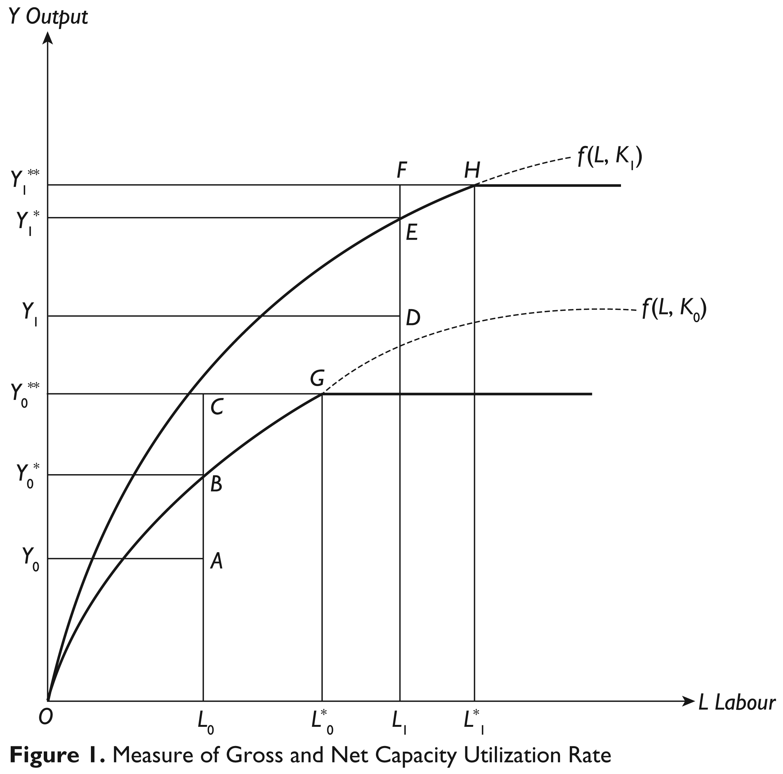
Suppose that a firm is producing output Y0 from the input bundle (L0, K0). This is shown by the point A. In that case, its technical efficiency is
The net measure of capacity utilization rate is
Similarly, for output Y1 produced from the input bundle (L1, K1) as shown by point D, technical efficiency is
The gross measure of capacity utilization rate is
Non-parametric Methodology to Estimate Total Factor Productivity Change and Capacity Utilization Rate
This article adopts the non-parametric method DEA introduced by Charnes et al. (1978) (CCR) and further generalized for variable returns to scale technology by Banker et al. (1984) (BCC) in order to measure ‘gross’ and ‘net’ capacity utilization rate.
Measurement of Technical Efficiency Using DEA
The major advantage of using DEA is that, unlike in the parametric approach, there is no need to specify any explicit functional form for the production function (for example, Cobb-Douglas or Translog) and mathematical programming techniques can be used to get point-wise estimates of the production function. In fact, DEA allows one to construct the production possibility set from observed input–output bundles on the basis of the following four assumptions:
All observed input–output combinations are feasible. The production possibility set is convex. Inputs are freely disposable. Outputs are freely disposable.
Now, consider an industry producing one output y from one input x. The input–output bundle (x, y) is considered as feasible if the output y can be produced from the input x. Let (xj, yj) represent the input–output bundle of firm j; and suppose that input–output data are observed for n firms. Then, based on the above assumptions, the production possibility set showing a variable returns to scale (VRS) technology is

Under the constant returns to scale (CRS) assumption, if any (x, y) is feasible, so is the bundle (kx, ky) for any k > 0. The production possibility set then becomes

One can measure the output-oriented technical efficiency TE(xs, ys) of a firm S by comparing its actual output ys with the maximum producible quantity from its observed input xs. Therefore, the output-oriented technical efficiency of firm S is

and T represents the production possibility set. 4
An alternative characterization of technical efficiency in terms of the Shephard Distance Function is
The standard non-parametric DEA model used to estimate output-oriented technical efficiency of a firm S, relative to a CRS frontier is


By imposing the additional restriction
Measurement of Biennial Malmquist Index of Total Factor Productivity
As mentioned above, this article primarily intends to examine the role of capacity utilization in explaining the variation in productivity growth rates across states over the period of 1970–1971 through 2007–2008. For the purpose we construct the Malmquist index of total factor productivity for Indian manufacturing using the state level input–output data. Although the detailed discussion on estimating productivity changes using DEA is available in Deb and Ray (2013), following paragraphs briefly describe the Malmquist index and its non-parametric estimation process.
Caves et al. (1982) define the Malmquist Productivity Index as the ratio of the period t and period t + 1 output-oriented Shephard distance functions pertaining to a certain benchmark technology. Equivalently, the Malmquist Index of total factor productivity of the firm S is

However, following Ray and Desli (1997), the decomposition of the Malmquist index, constructed in this manner, may result in linear programming infeasibilities for some observations while estimating the scale efficiency change. In order to avoid this problem we construct the Biennial Malmquist index using a revised procedure introduced by Pastor et al. (2011). Instead of using a contemporaneous production possibility frontier, we estimate the technical efficiency of a production unit with reference to a biennial production possibility frontier. Using the output-oriented technical efficiency scores with reference to a CRS biennial frontier, the Biennial Malmquist Productivity Index of the firm S producing a single output from multiple inputs is measured as

The appropriate DEA model to estimate period t output-oriented technical efficiency


where nk is the number of observed firms in period k and
Period t output-oriented technical efficiency

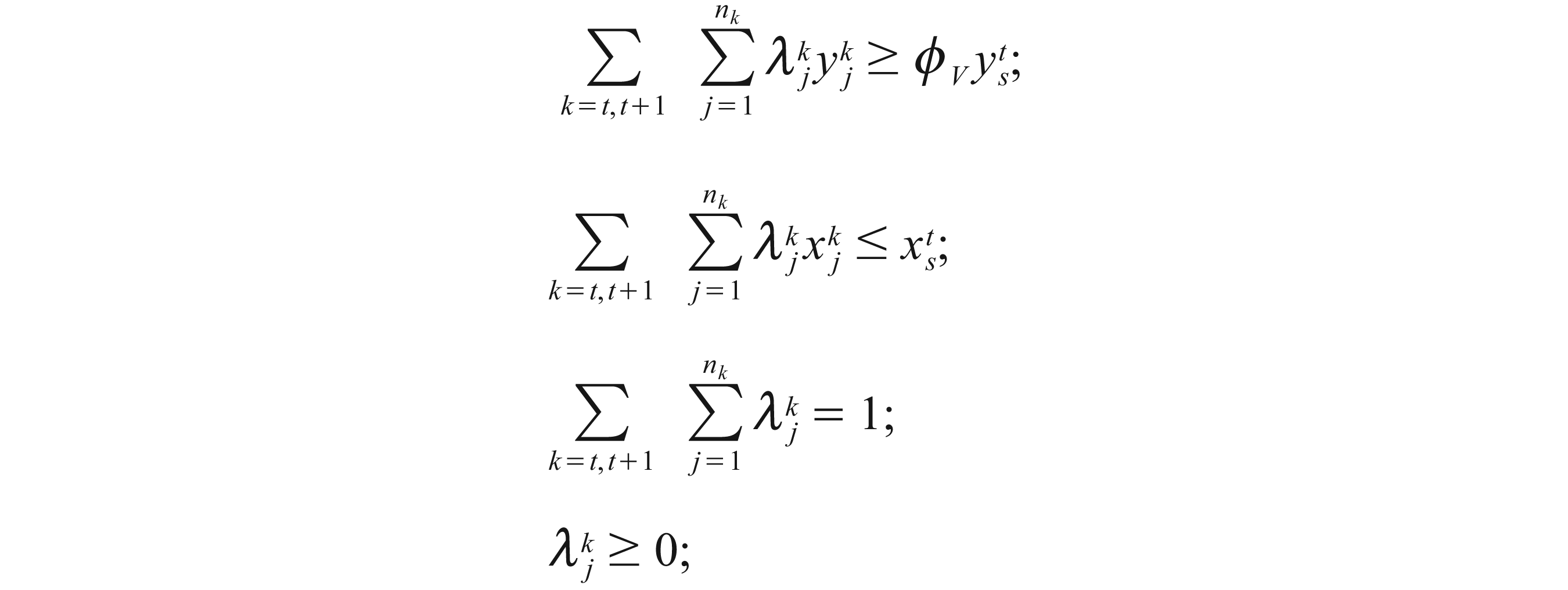
where nk is the number of observed firms in period k and
Measurement of Change in Capacity Utilization Rate Using DEA
Färe et al. (1989) developed a non-parametric (linear programming) framework in which physical capacity and a measure of the capacity utilization rate can be determined from data on observed inputs and outputs.
Suppose that

Following Banker et al. (1984) for the input–output bundle


Further, as shown by Färe et al. (1989),


Note that because the vector of variable inputs x in the constraint is itself unrestricted, there is effectively no constraint on these inputs.
We measure technically efficient output and capacity output by solving model (16) and (17) respectively, with respect to a production possibility frontier which is constructed by pooling input–output data for two adjacent years.
5
Accordingly capacity utilization index measuring rate of change in capacity utilization for the firm S becomes

Data and Empirical Application
Using the state level input–output data obtained from ASI, we compute the measure of gross capacity utilization rate (gcur) and the measure of net capacity utilization rate (ncur) for Indian manufacturing for the period 1970–1971 through 2007–2008. The period from 1970–1971 through 1991–1992 is treated as the pre-reform period and the remaining years are considered as the post-reform years. Twenty major states are covered in this study and these states together produce 91 per cent of the total manufacturing output, and generate 93 per cent of the total manufacturing employment in 2007–2008.
The DEA models discussed conceptualize a single-output, five-input production technology for the manufacturing industry in India. The inputs considered are: (a) capital; (b) non-production workers; (c) production workers; (d) raw materials; and (e) energy. 6
The input–output data reported in the ASI for individual states are aggregates over all firms in the state covered by the survey. Even though, the actual input–output quantities of the individual firms are all feasible bundles, the total input–output bundle—the sum of those feasible bundles—is neither observed nor a weighted average of feasible observations. This aggregation poses a serious technical problem and applying DEA to this data violates underlying assumption for constructing production possibility frontier. Assumptions of constant returns to scale along with convexity of the production possibility set would ensure the feasibility of these aggregate input-output bundles. Nevertheless, the assumption—a reference technology showing CRS throughout the production process—is quite restrictive for such an analysis. Therefore, in order to avoid this aggregation problem we use the average input–output bundle for any state as a feasible combination and as a basis for constructing the non-parametric production possibility frontier.
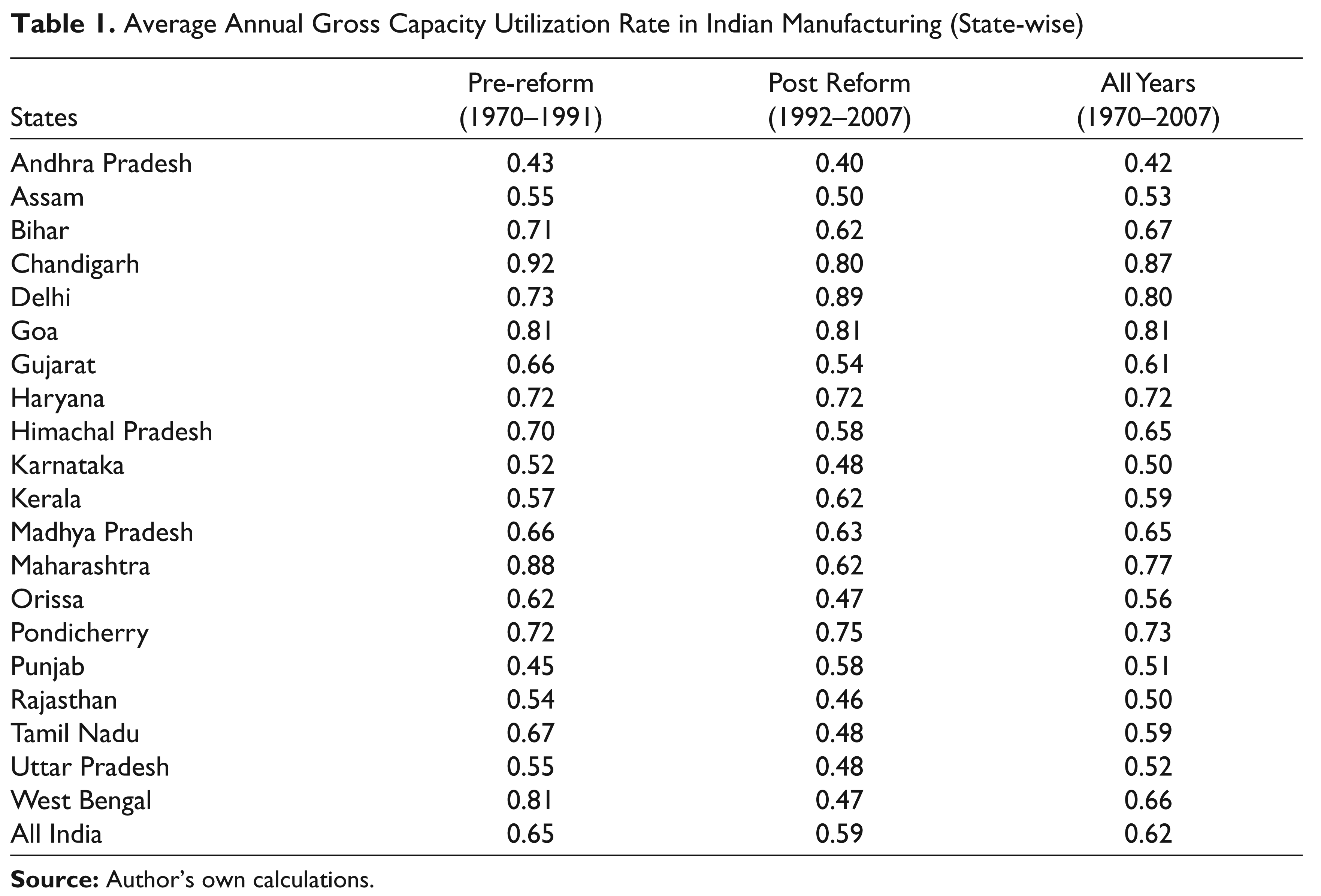
Average Annual Gross Capacity Utilization Rate in Indian Manufacturing (State-wise)
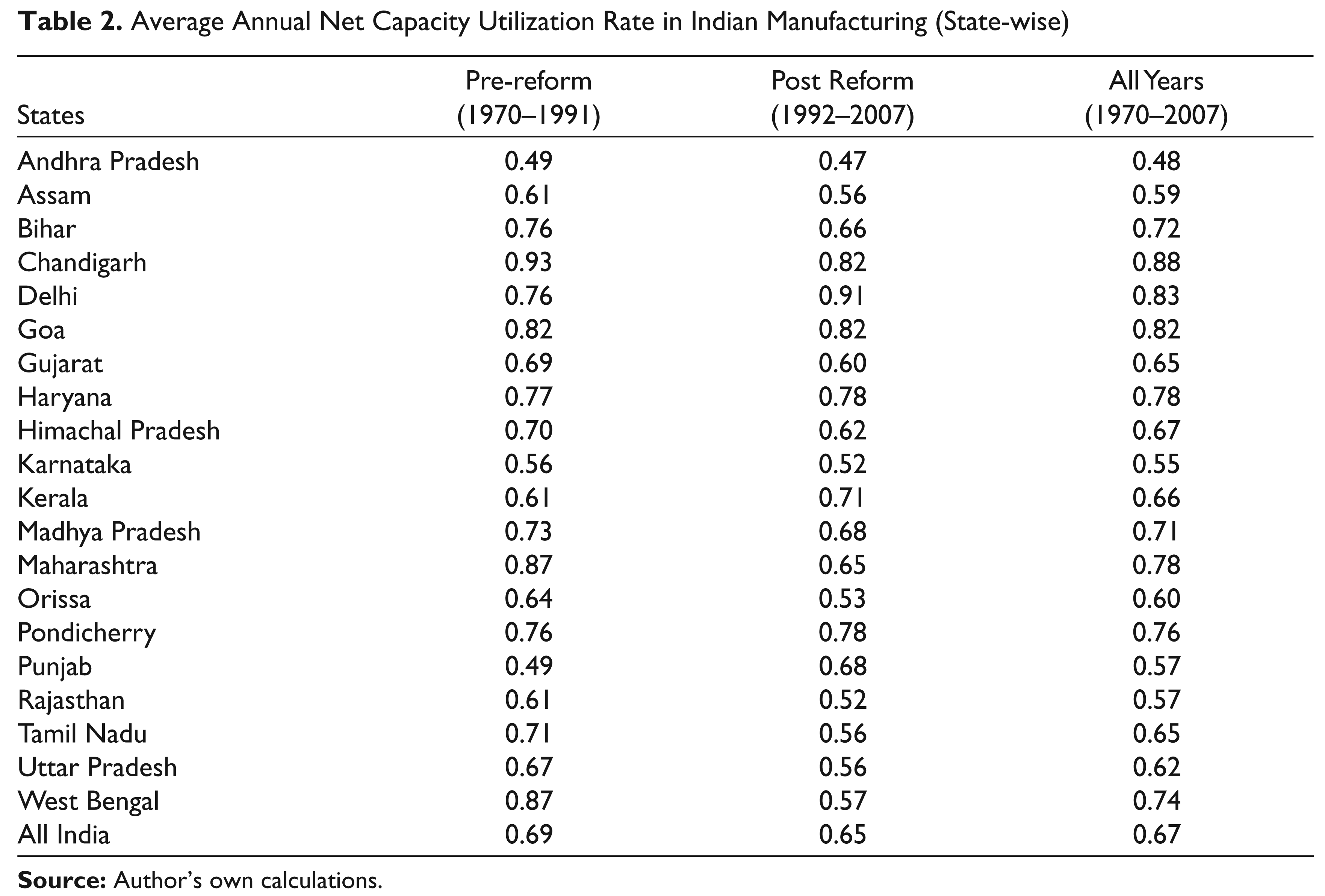
Average Annual Net Capacity Utilization Rate in Indian Manufacturing (State-wise)
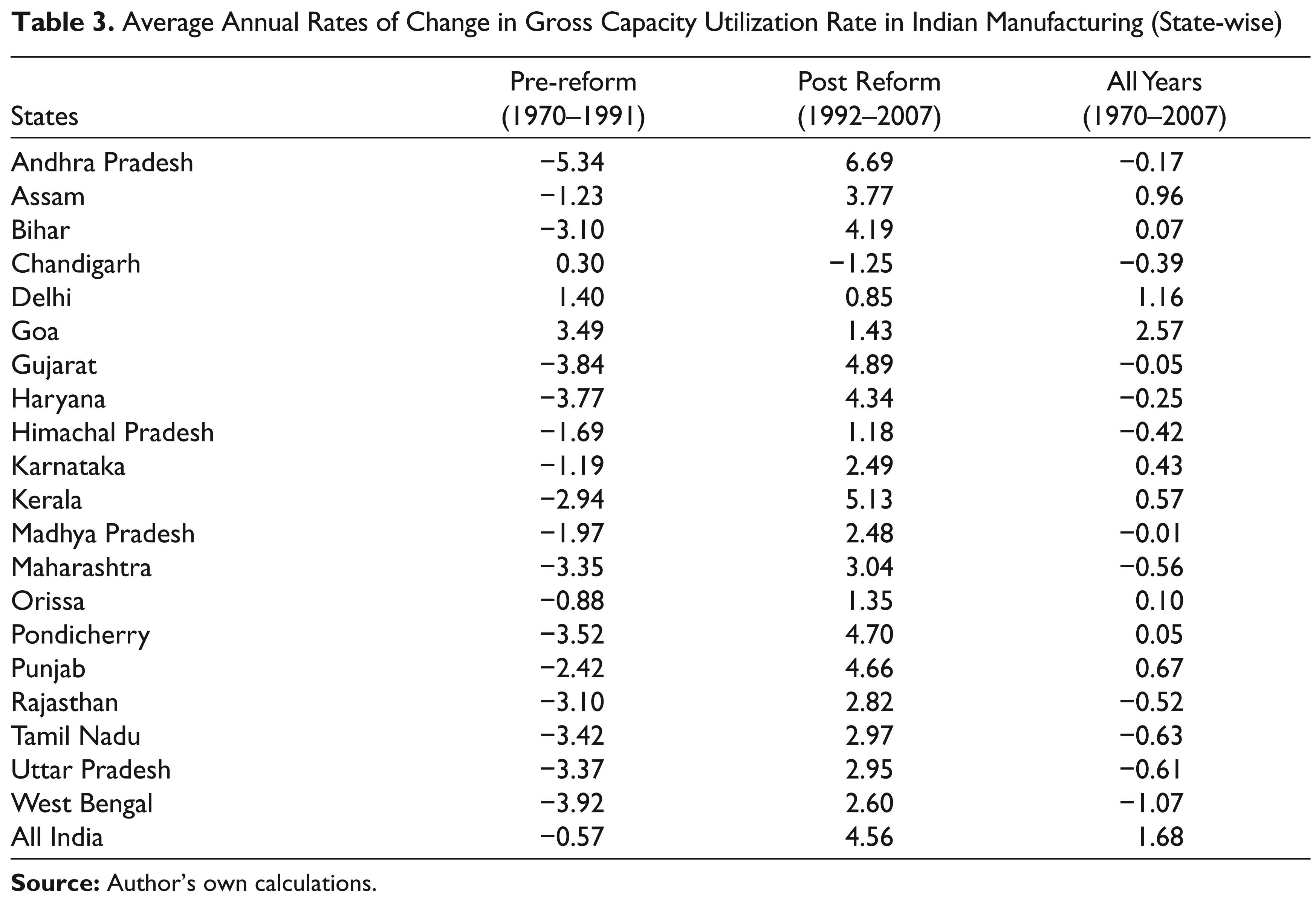
Average Annual Rates of Change in Gross Capacity Utilization Rate in Indian Manufacturing (State-wise)
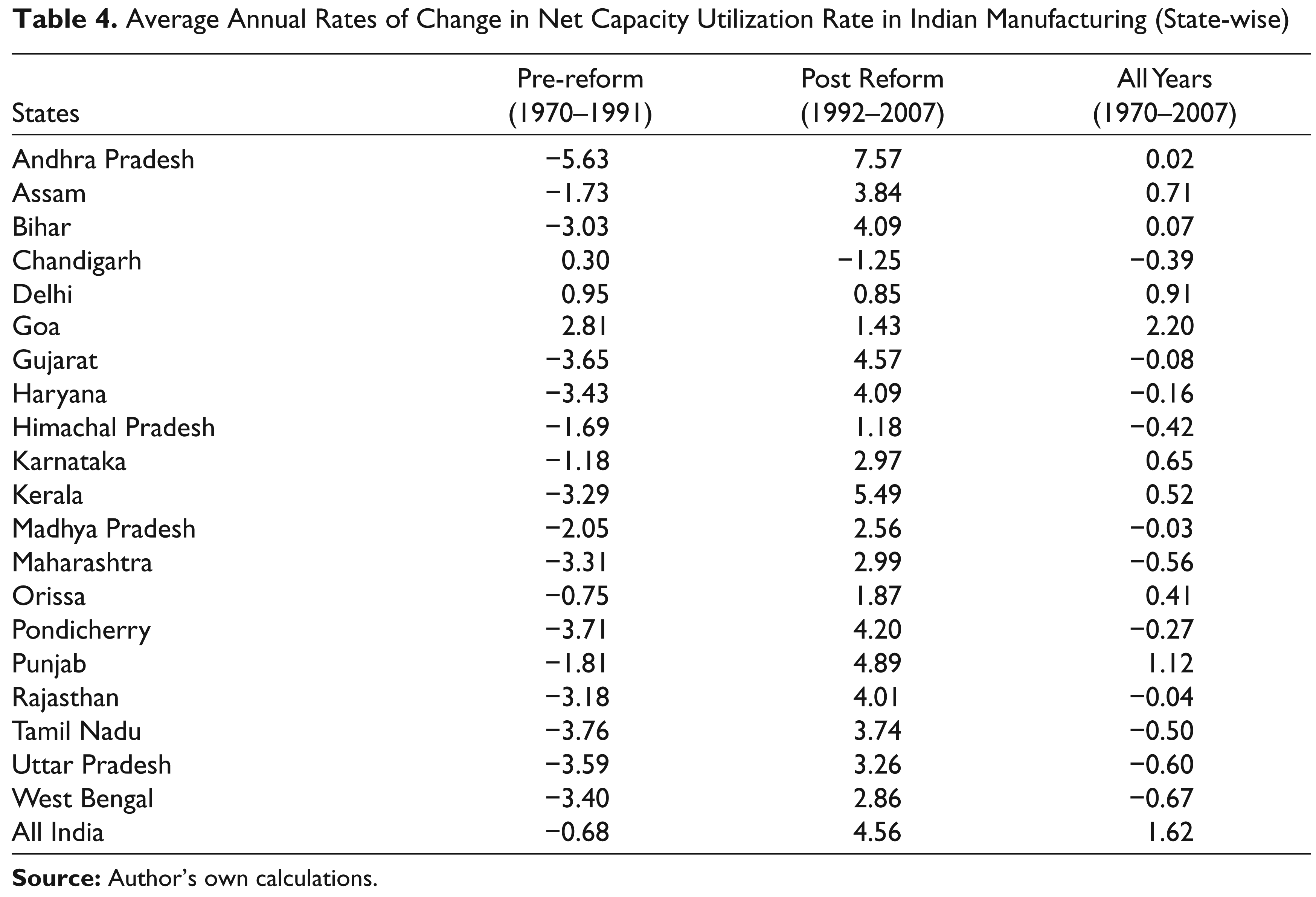
Average Annual Rates of Change in Net Capacity Utilization Rate in Indian Manufacturing (State-wise)
Empirical Estimates of Capacity Utilization Rate and Capacity Utilization Growth
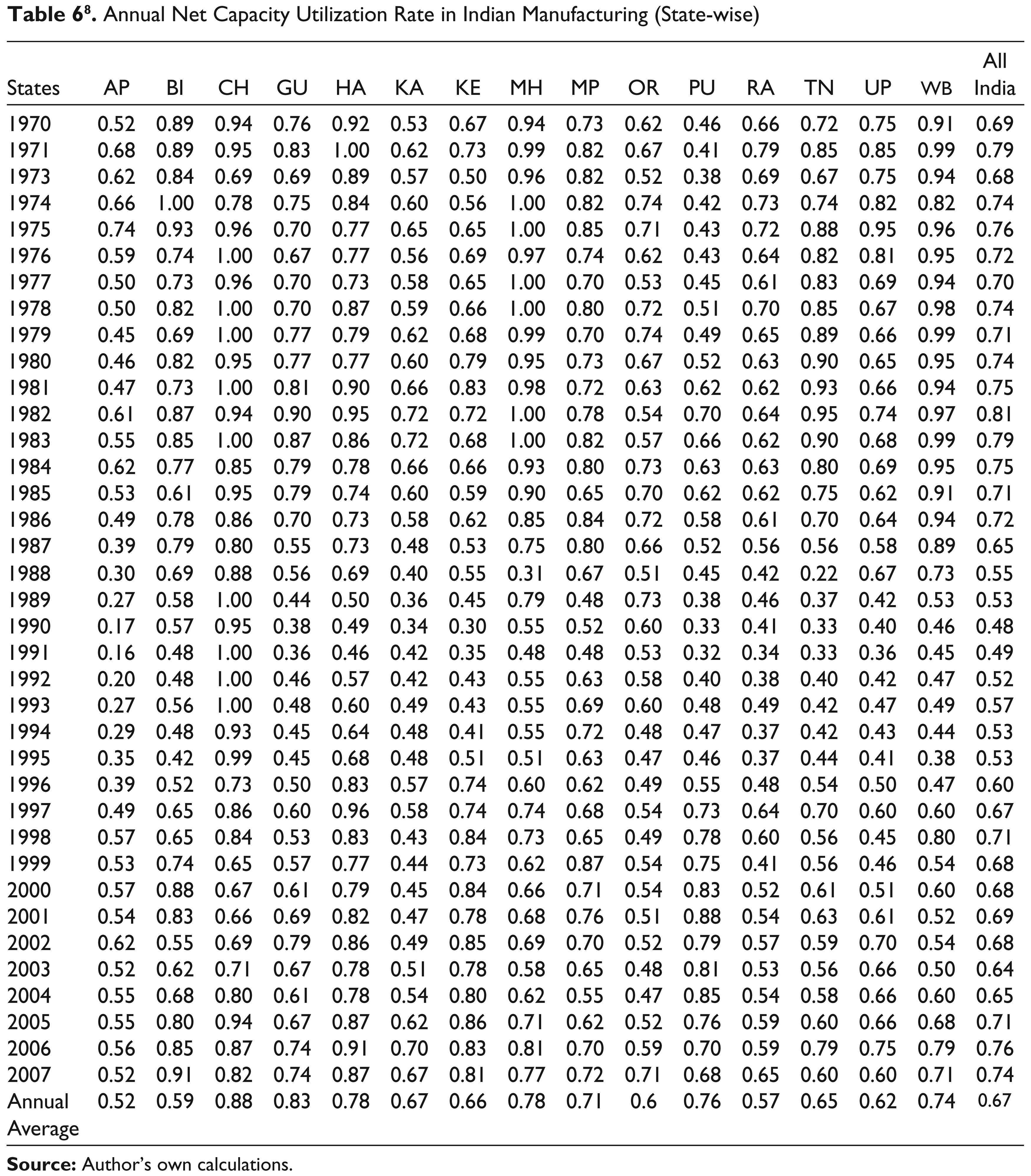
In Tables 1 and 2 we report the annual averages of these two measures at the All-India as well as at the state level. Also in Tables 3 and 4 we provide state-wise estimates of rates of change in gross and net capacity utilization rate for the pre-reform as well as for the post-reform years.
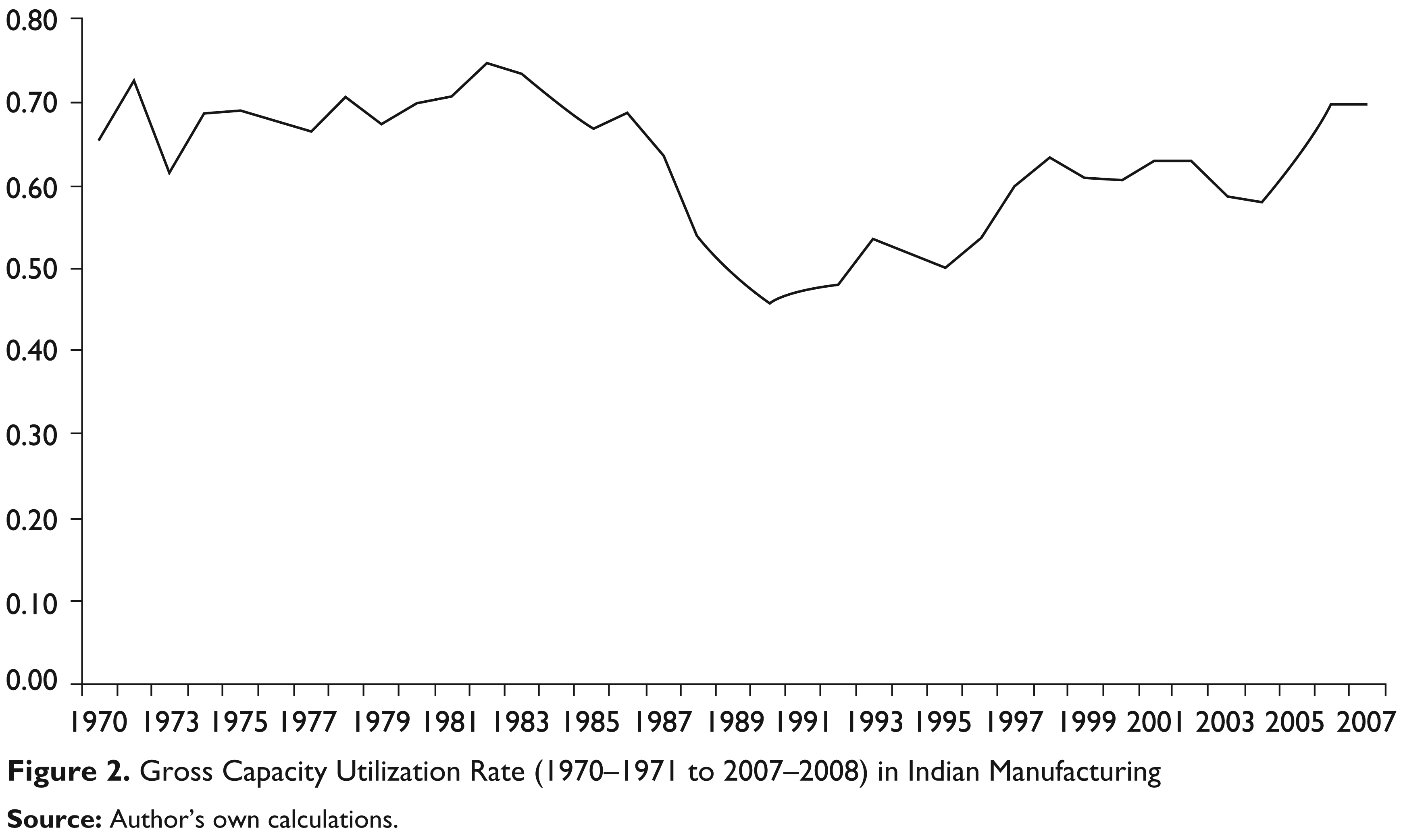
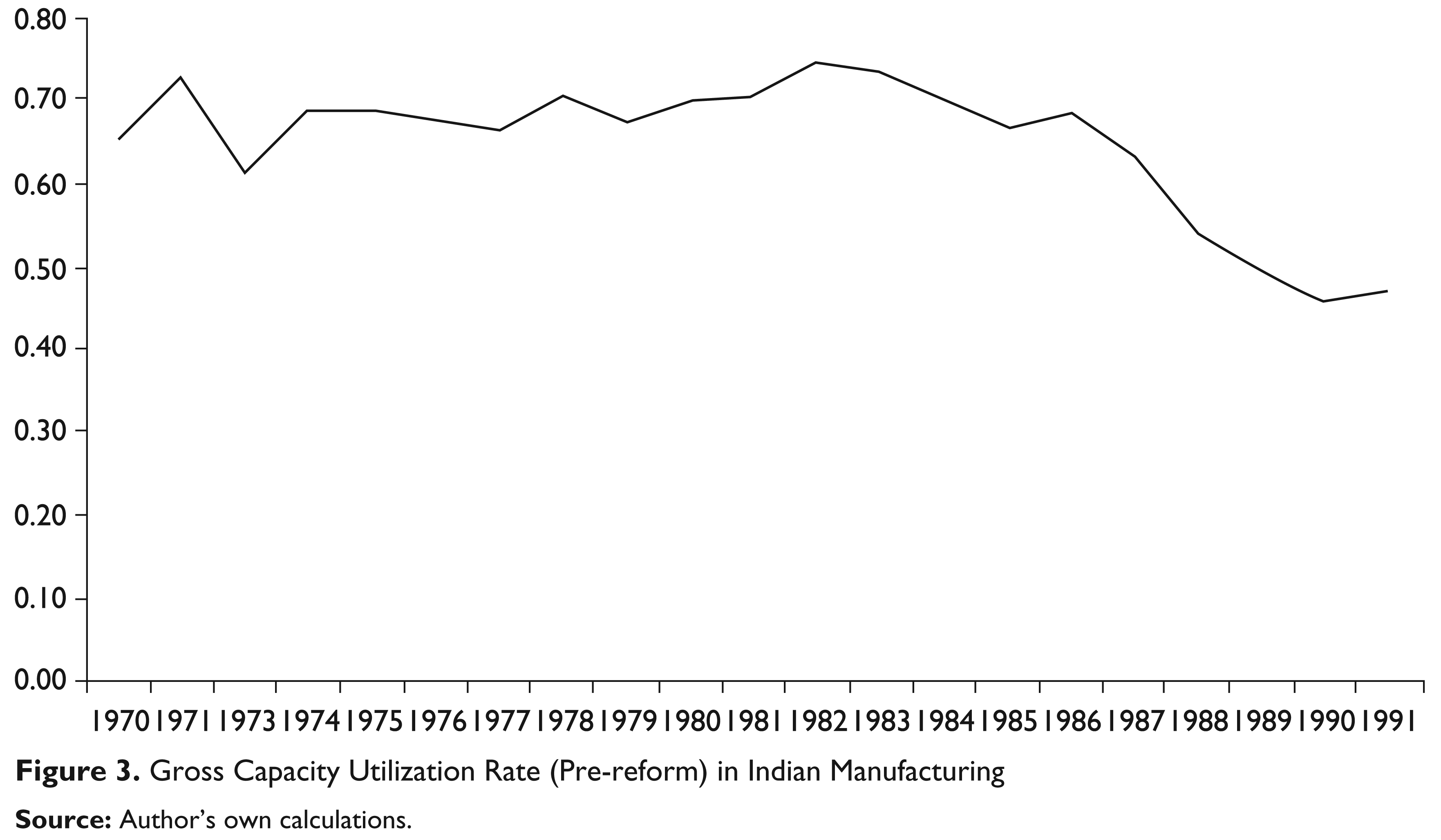
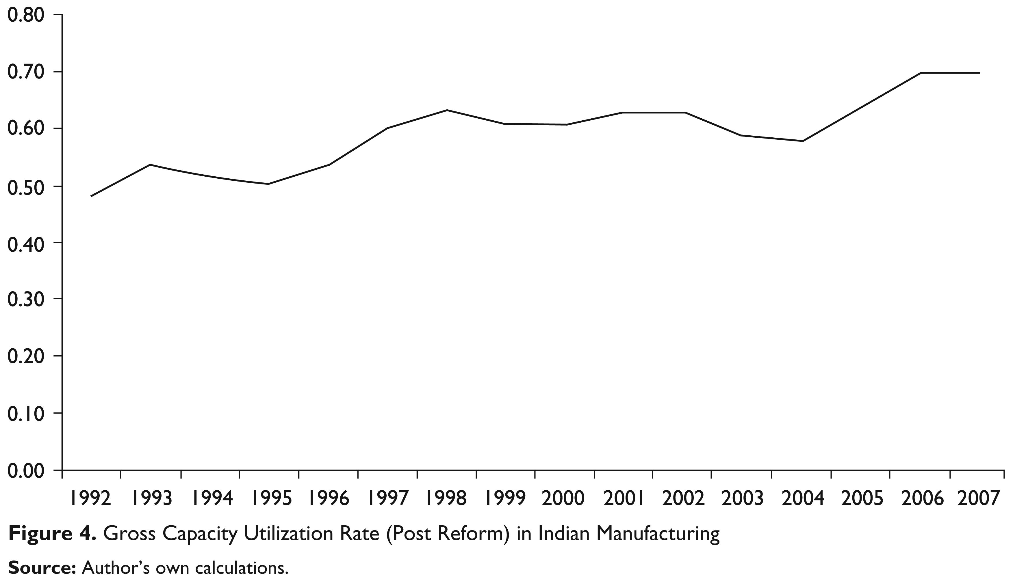
Estimates of rates of change in gross capacity utilization in total manufacturing show that, at the all-India level the capacity utilization rate improved by 1.68 per cent per year during the entire sample period. We also observe that during the entire study period, on a year-to-year average Indian manufacturing utilized 62 per cent of its capacity at the national level. Over the years 1970–1971 through 1991–1992 average capacity utilization rates was 65 per cent per year. However, during this period the annual capacity utilization rate showed a steady downward trend (see Figure 3) and declined by around 0.6 per cent per year. The year-wise analysis (see Table 5 and Figure 2) reveals that there is continuous decline in capacity utilization rate during the period of 1982–1983 to 1990–1991. In the year 1982–1983 capacity utilization rates reached its peak of 75 per cent. The lowest rate of 46 per cent was attended in 1990–1991. One possible explanation for this sharp decline, mainly during the latter part of this period, is increasing labour dispute in Indian states. The average duration of lockouts and strikes increased considerably in the 1980s and consistently remained high relative to that in the previous decades (see Shyam Sundar, 2004) for detailed statistics on labour dispute in this period). Saha and Pan (1994) characterized this latter part of the 1980s as the period of ‘lock-out dominance’. Even though Indian manufacturing started to get access to better access to capital goods during this period the restricted availability of labour input possibly explains the underutilization of capital inputs. Because annual capacity utilization rate reached the lowest in 1990–1991, in spite of the fact that it started to grow at the rate of 4.56 per cent per year, the annual average dropped to 59 per cent over the post-reform period (Figure 4).
From state-level estimates of capacity utilization rate we observe that on an average, manufacturing sectors in Chandigarh, Delhi and Goa were able to utilize more than 80 per cent of plant capacity over the entire study period. Maharashtra comes next. Over the entire sample period, in Maharashtra a high capacity utilization rate of 77 per cent is observed. However, it should be noted that in 1990–1991 Maharashtra experienced a substantial decline. Relative to other states on an annual average Andhra Pradesh utilized the minimum plant capacity of 42 per cent during this period. Among other major industrial states both in Gujarat and Tamil Nadu around 60 per cent of plant capacity has been utilized during this period.
For most states capacity utilization rate declined over the pre-reform years. However, a noteworthy aspect of these pre-reform estimates at the state level is the steady decline in capacity utilization rate in West Bengal over the years 1970–1971 through 1990–1991. The annual capacity utilization rate of 90 per cent in 1970–1971 dropped to 40 per cent in 1990–1991. It should be noted that during this period West Bengal accounted for more than 60 per cent of total workdays lost in India (Shyam Sundar, 2004). Along with labour dispute, successive closures of industrial units (partially due to labour unrest) during this period possibly explain the observed decline in plant capacity utilization rate in this state. As discussed in Deb and Ray (2013), during this period annual average manufacturing productivity in West Bengal also declined substantially.
7 Annual Gross Capacity Utilization Rate in Indian Manufacturing (State-wise)
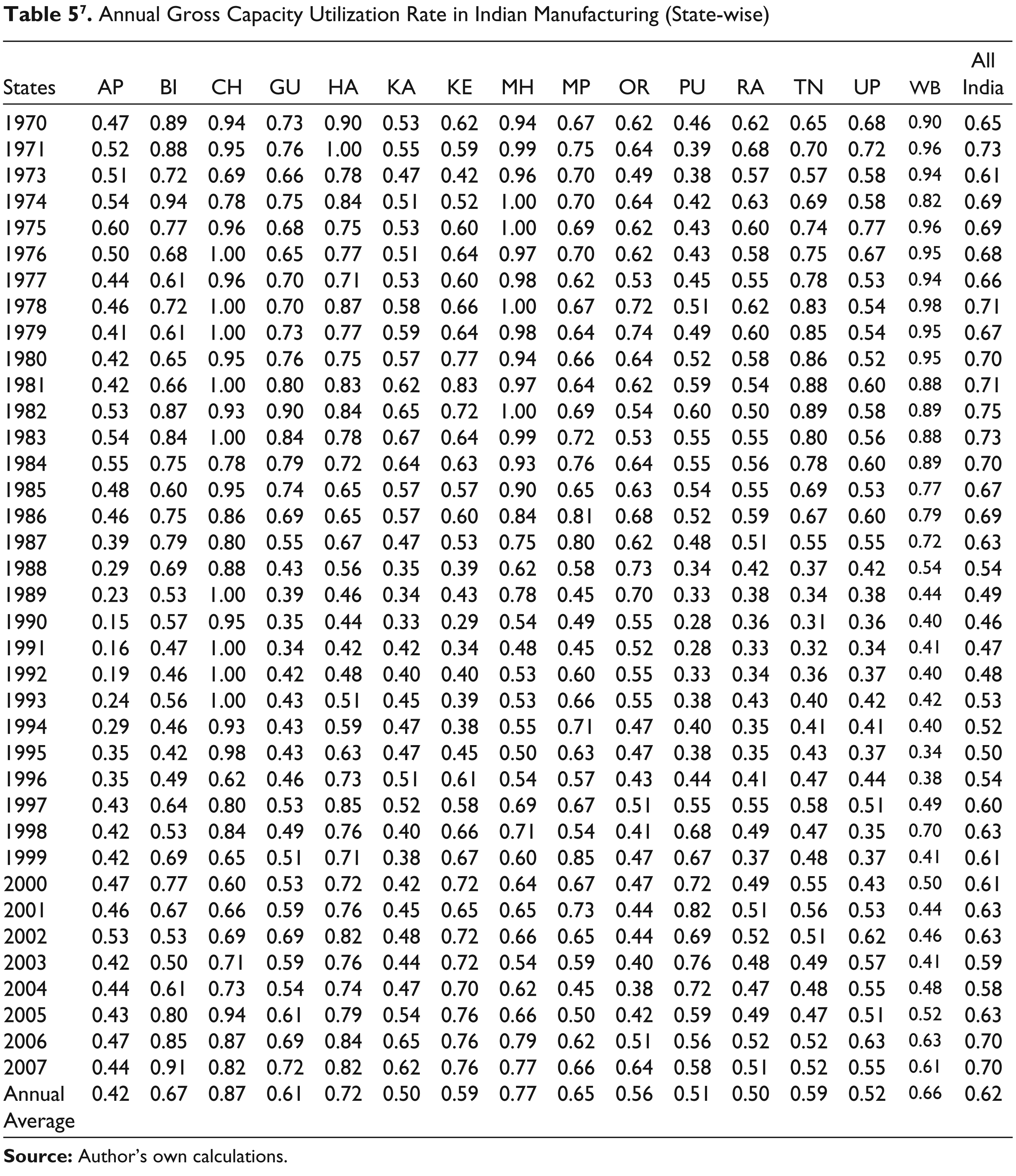
Over the entire post-reform period in most states average annual capacity utilization rate became lower. However, the capacity utilization growth rates for these states substantially improved after the reforms. Noticeable improvement was observed for the major states including Andhra Pradesh, Bihar, Gujarat, Maharashtra, Tamil Nadu and West Bengal. Since West Bengal experienced a decline in capacity utilization rate by around 4 per cent per year before the reforms, even though it grew by around 3 per cent per year after the reforms, the average annual capacity utilization rate in this state became around 57 per cent which was lower than its pre-reform estimates by more than 25 percentage points.
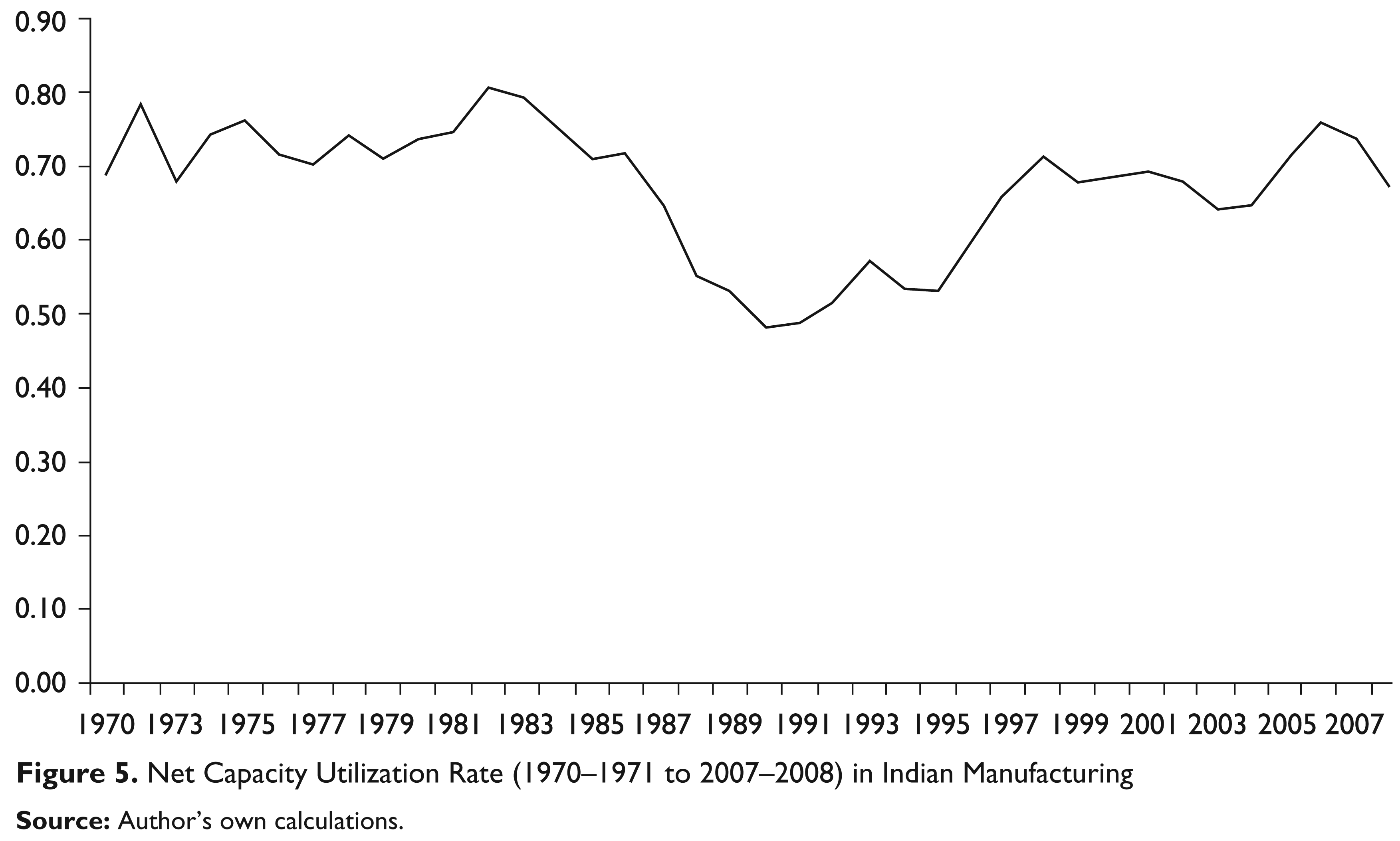
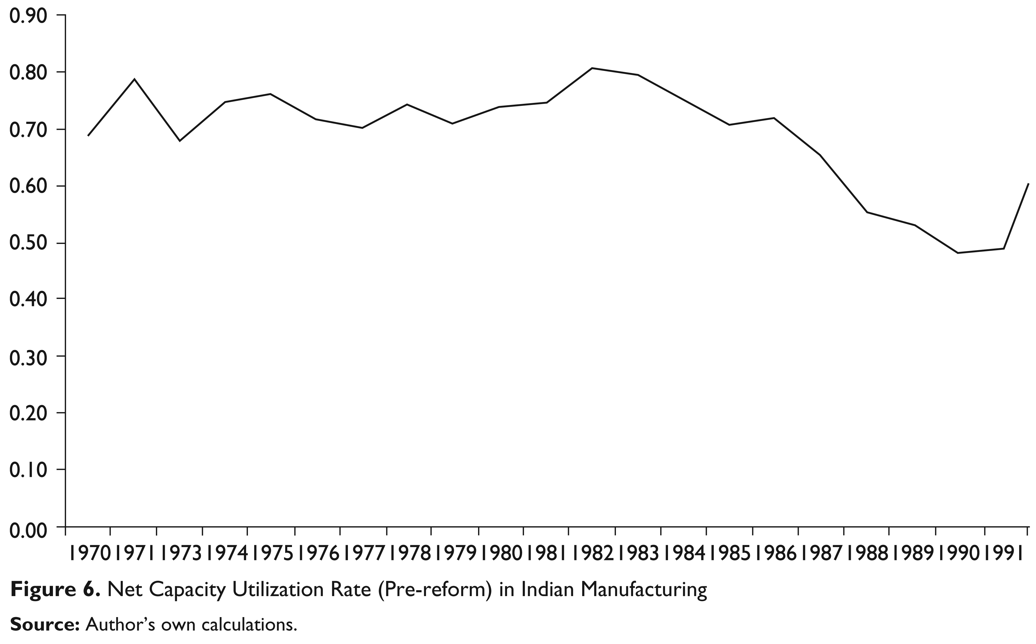
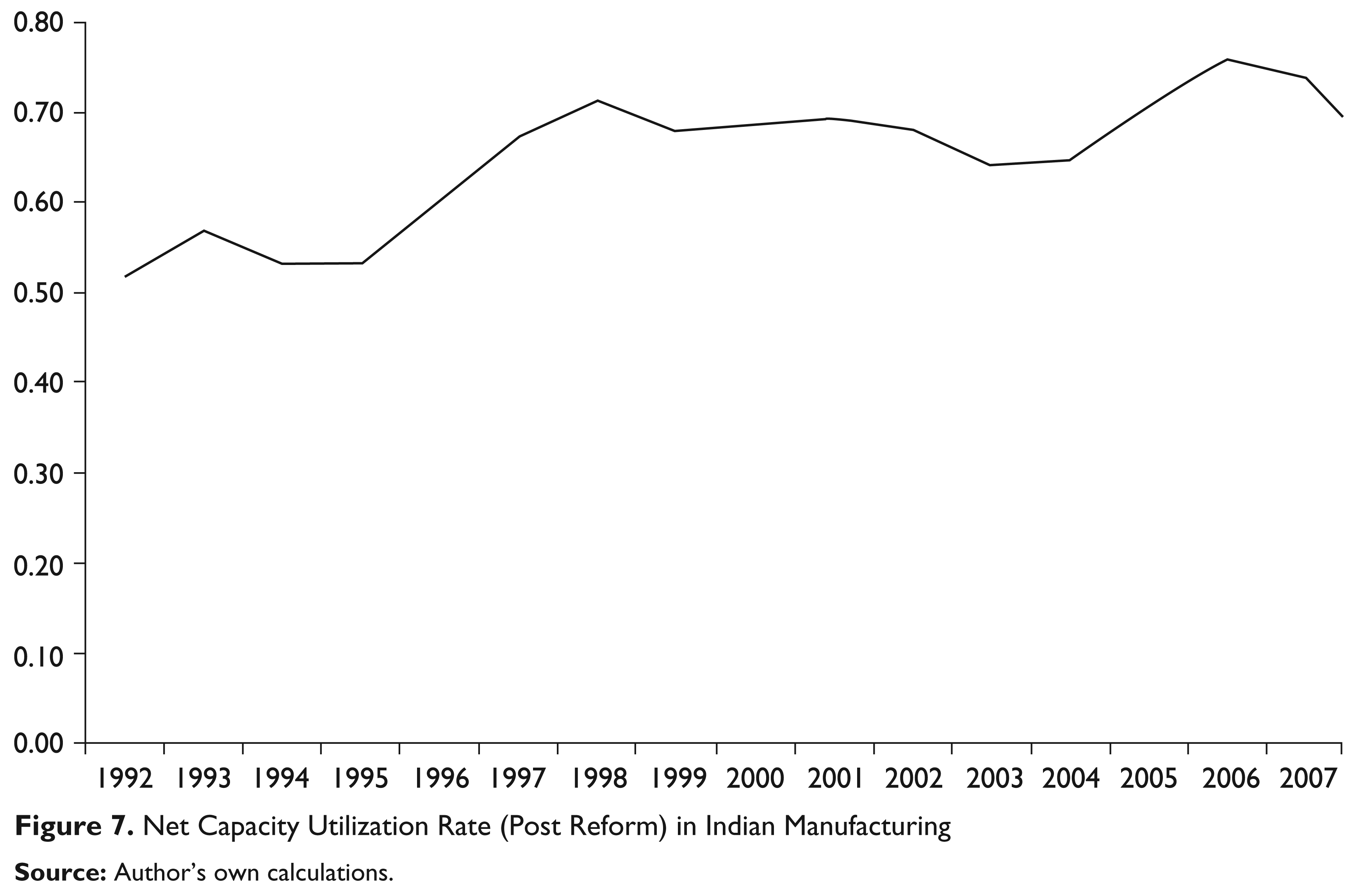
Estimates of net capacity utilization rates (see Tables 2, 4 and 5 and Figures 5, 6 and 7) reveal a trend similar to what we observe from the estimates of gross capacity utilization rate both at the state and the national level. However, estimates from these two measures are substantially different reflecting the level of technical inefficiency or wasted capacity in Indian manufacturing. Also we find that growth rate in net capacity utilization (see Table 6) in post-reform period was substantially higher at the national as well as at the state level.
8 Annual Net Capacity Utilization Rate in Indian Manufacturing (State-wise)
Regression Analysis
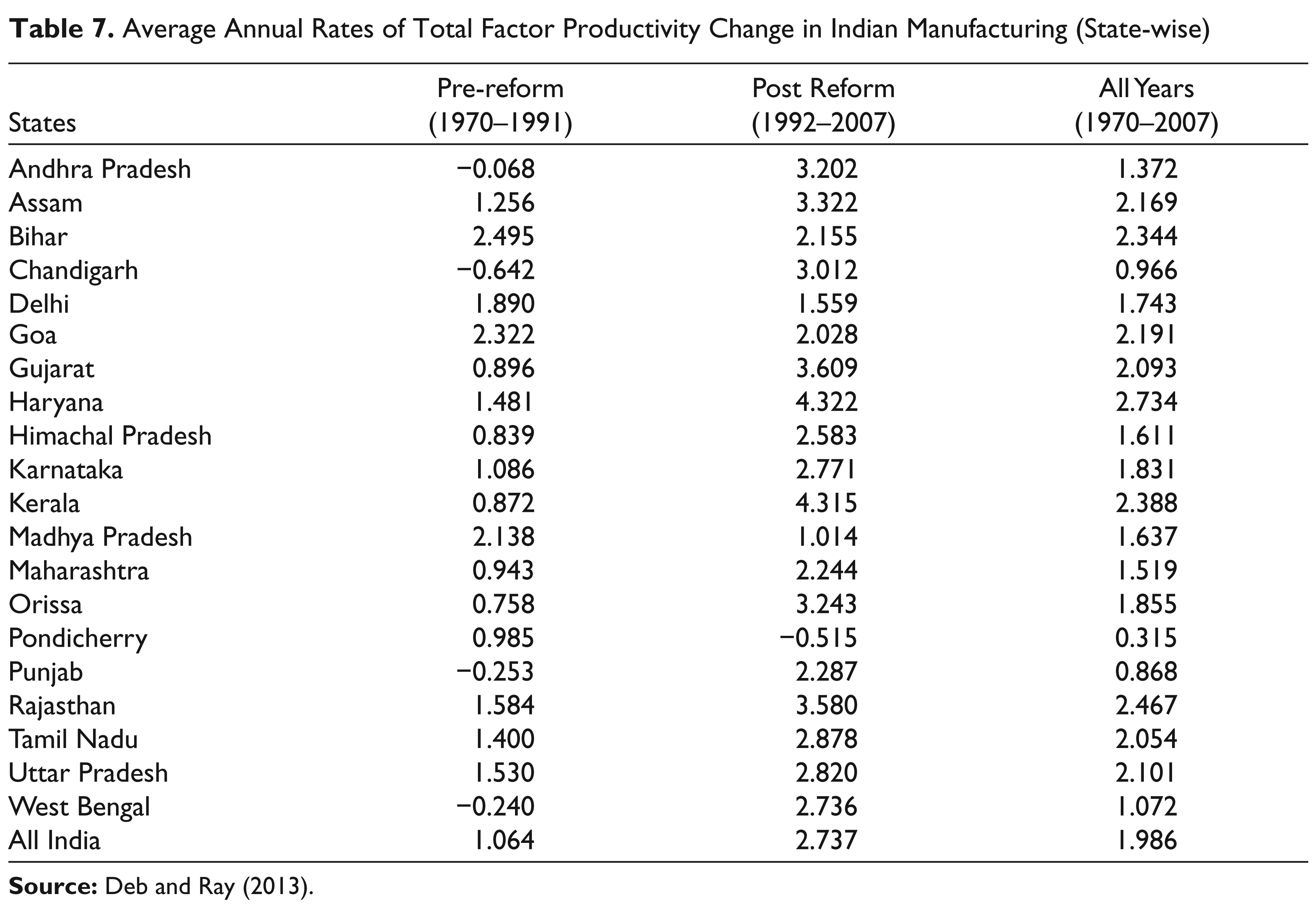
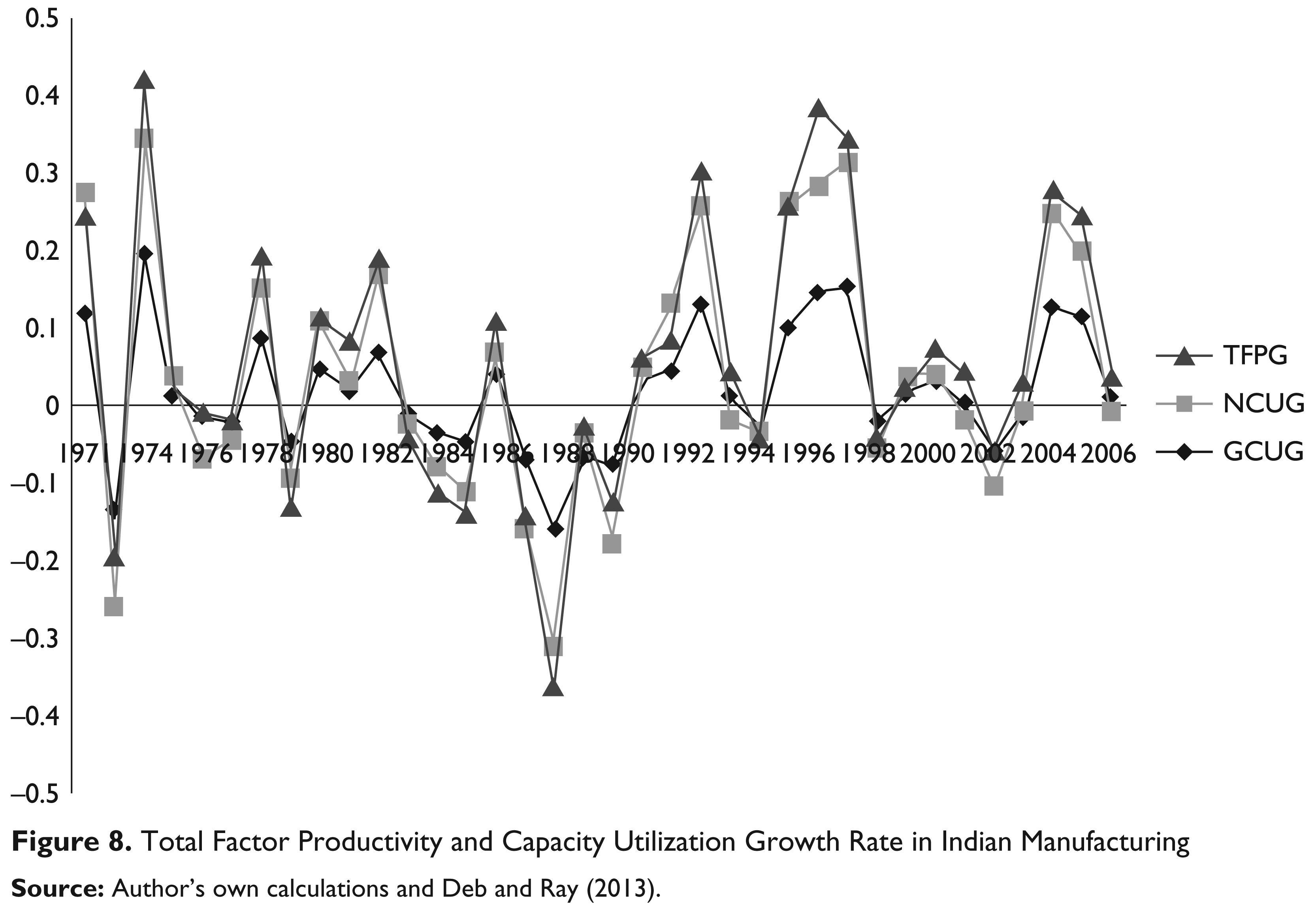
The empirical estimates of rates of productivity change presented in Table 7 show that at the individual level, most states enjoyed faster productivity growth after the reform. Despite the fact that some states experienced a slowdown in productivity growth or even a productivity decline after the reforms, manufacturing productivity grew faster during the post-reform period at the national level. Moreover, from Figure 8 we can see that both total factor productivity and capacity utilization rate followed similar growth path over the entire sample period at the national level.
Average Annual Rates of Total Factor Productivity Change in Indian Manufacturing (State-wise)
Given the pro-cyclical nature of productivity, enhancement in plant capacity utilization through stimulation in demand for and removal of infrastructural bottlenecks in manufacturing production during the post-reform years could be the principal factor behind the observed acceleration in productivity growth in Indian manufacturing. If the impacts of economic reforms were channelized through a higher capacity utilization rate, no additional impact of reforms would be detected in a regression model once annual rates of change in capacity utilization was included as an explanatory variables. On the other hand, if other kinds of structural changes, as mentioned before, from the reforms improved productivity, a simple dummy variable signifying the era of economic liberalization would come out to be statistically significant.
Therefore, to identify the role of economic reforms and capacity utilization growth in enhancing the productivity growth we estimate the following regression model using the information on productivity and capacity utilization growth for 20 major Indian states over the period 1970–1971 through 2007–2008:

for
The dependent variable tfpgit is the rate of change in total factor productivity in manufacturing for ith state in year t and is calculated as

where mpiit is the Malmquist Index of total factor productivity for ith state in year t.
To capture the marginal effect of reforms on productivity change in Indian manufacturing we include the qualitative variable reft in our econometric model. The dummy variable reft assumes the value 0 in the pre-reform period and 1 for the post-reform years.
The other explanatory variable cugit is the rate of change in capacity utilization for state i in year t and is calculated as

where cuiit is the index of capacity utilization rate for ith state in year t.
There are some state specific time invariant factors such as geographical location, work culture, and political climate which may influence productivity growth rate. Therefore, we include state-specific factor ni into our model to capture possible unobserved heterogeneity across states. These factors are also very likely to be correlated with the capacity utilization growth rates in different states. So we estimate a one-way fixed effect model by the within-effects estimation technique.
The estimated coefficients in the model are reported in Table 8. We examine the impact of both gross and net capacity utilization growth rate separately by estimating the specified regression model. Regression results show that the gross capacity utilization growth rate is positively related to productivity growth rate. For 1 per cent growth in gross capacity utilization rate, productivity growth rate is expected to increase by 0.16 per cent per year. Moreover, this marginal impact of gross capacity utilization growth rate is statistically significant at 1 per cent level.
On the other hand, even though the estimated regression coefficient implies that productivity growth rate increases by 0.02 per cent when net capacity utilization growth rate increases by 1 per cent, this impact is not statistically significant at 5 per cent or even at 10 per cent level. In fact, it has a p-value of 0.148.
Regression Results
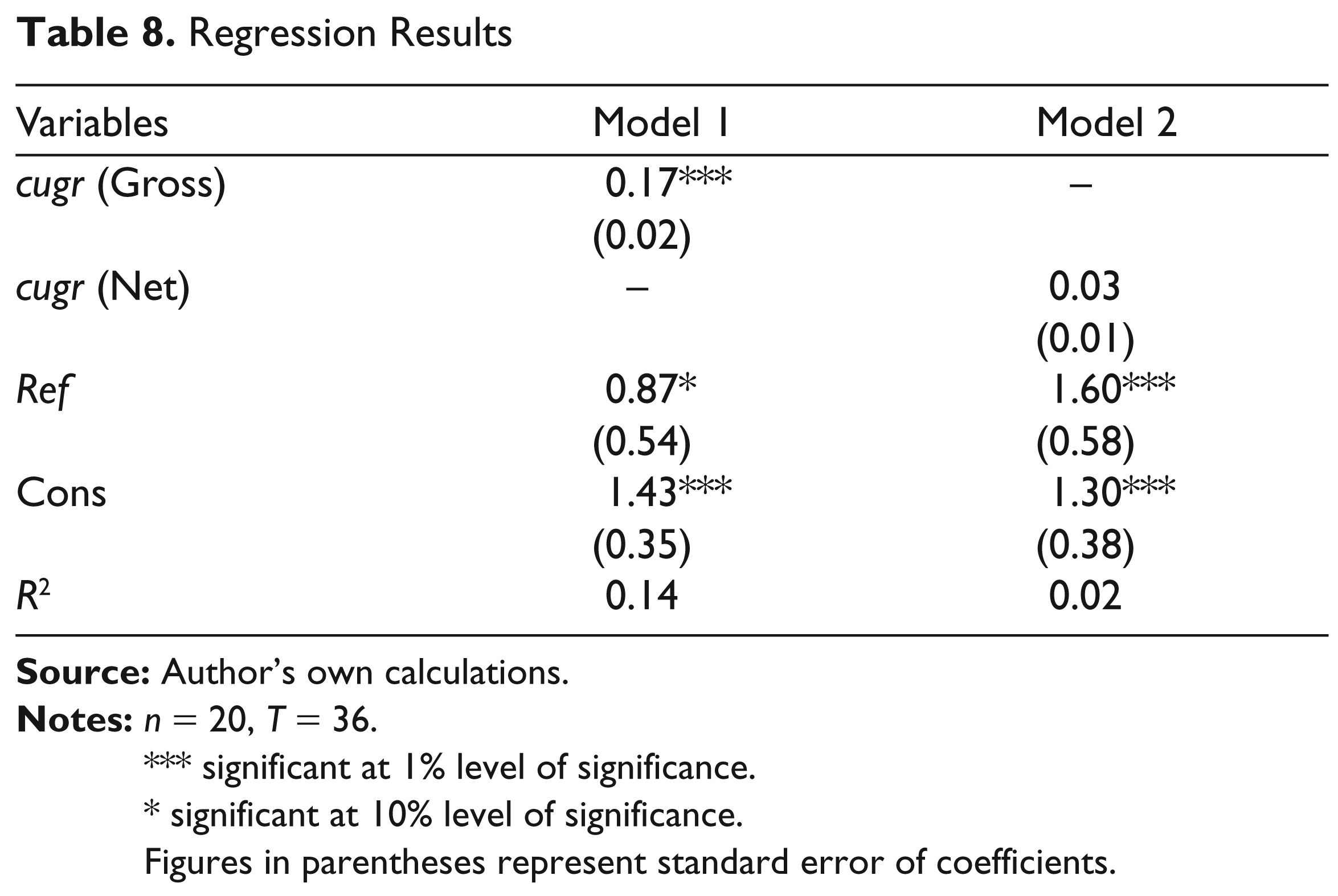
*** significant at 1% level of significance.
* significant at 10% level of significance.
Figures in parentheses represent standard error of coefficients.
These results confirm that the better capacity utilization (presumably through demand stimulation and better access to essential inputs for production such as raw materials and capital goods) led to acceleration in manufacturing productivity growth over the post-reform years.
The coefficient of reft is positive showing that on average manufacturing productivity grew faster over the post-reform years even when capacity utilization is explicitly accounted for. When we control for of gross capacity utilization growth rate, estimated coefficient of reft shows that after the year 1991 productivity growth rate increased by 0.88 per cent. This result is statistically significant at the 10 per cent level. We find a stronger effect of economic reforms when we use net measure of capacity utilization growth rate as the other explanatory variable. The estimated coefficient shows that on average, total factor productivity growth rate in Indian manufacturing is higher by 1.6 per cent per year after the reforms. This result is significant at 1 per cent level of significance.
The difference in the results across these two models is possibly due to the difference in the ways of measuring net and gross capacity utilization rate. The difference between net and gross capacity utilization rate is due to the difference resulting from including and not including the wasted capacity through technical inefficiency. So when we use net capacity utilization growth rate as an explanatory variable, then the technical inefficiency is captured by reforms. This possibly explains the stronger impact of reforms in the second model. Actually reform is enhancing productivity growth through improvement in technical efficiency.
Conclusion
In this article we examine if all the impact of economic reforms of 1991 is channelled through better capacity utilization alone. We argued that structural changes resulting from reforms and better plant capacity utilization in manufacturing could be two possible (but not mutually exclusive) explanations for this accelerated productivity growth. Using the method of DEA we compute gross and net capacity utilization growth rate from the input–output data for major Indian states over the period 1970–1971 through 2007–2008. Empirical estimates of capacity utilization rates show that during the post-reform years annual average capacity utilization rate is lower for most of the states as well as for the country as a whole. However, after the reforms capacity utilization displayed a steady upward trend and growth rate in capacity utilization is substantially higher both at state and at the national level. A subsequent regression analysis confirms that there was evidence of a favourable impact of economic reforms on productivity growth in total manufacturing, beyond the positive impact of improved capacity utilization. Therefore, better utilization of plant capacity can be considered as an important factor in enhancing the productivity growth of a firm. Thus it is a managerial challenge for a firm to produce the capacity output and increase the capacity utilization rate so as to push up the firm to higher growth path.