An Alternative Analysis of Scale Data: A Marketing Application

Abstract

The idea of materialism is one of the most important in modern consumer behaviour literature. In this article we have attempted at studying this component using the celebrated Richins and Dawson (1992) scale, where the required data has been collected using the standard instrument. This data is analyzed with the help of the mechanisms of item response theory (IRT). Specifically the graded response model has been used to analyze and get an insight into the problem of subjective well-being. Item response theory is an increasingly popular approach for development, evaluation and administration of psychological measures. We have used in this article one of the three IRT fundamentals, namely, the item response functions. We next illustrate how IRT modelling can be put to use to analyze the data collected in the study of the judgement component of subjective well-being. To that end, we have used the grm() function available in R. The results obtained are thereafter interpreted.

Keywords

Scale data Cronbach’s alpha classical test theory item response theory

Introduction

Traditional scaling procedures based on reliability measures have received the most attention for attitude scaling in the marketing research literature as evidenced by their rampant use in all marketing articles and go beyond the scope of any possible literature review. The advent of standard computer algorithms and even downloadable software patches enable researchers to accomplish standard analyses of marketing data. However, standardization often lead to loss of, what we term here as, data sensitivity.

Fundamentally, these procedures assume a constant standard error of measurement along the attitude continuum, that is, reliability only indicates the overall efficiency of the scale across all attitude levels. Though the correlation of an item with the scale may help in choosing items that contribute the most to the scale, it is hard to decipher whether these items contribute to the discerning ability at the high or low ends of the attitude scale. In addition, traditional procedures do not provide a measure for the specific contribution of each response category for measurement accuracy. For example, for Likert-type items, does ‘strongly agree’ provide more information than ‘agree’, given the item, along the attitude scale? In this article we present approaches based on multi-method distribution free approach which allow the researcher to select items on the basis of their ability along the attitude continuum.

The data for the study were collected through a structured survey conducted in India using Richins and Dawson’s (1992) materialism scale. Since its inception, the scale has been used in numerous studies in USA and elsewhere, and there now exists a substantial base of information about the psychometric properties of this scale and about its relationship to other consumer constructs. Materialism continues to be of great interest to scholars, social commentators and public policy makers. Since 1992, more than 100 empirical studies have examined materialism, and countless articles in the popular press have discussed materialism in contemporary societies. Given the interest in this construct, a re-examination of materialism and its measurement seems appropriate, especially in the context of an emerging market where materialism is supposed to be expanding.

Richins and Dawson define materialism as the importance ascribed to the ownership and acquisition of material goods in achieving major life goals or desired states, and they conceptualize material values as encompassing three domains: the use of possessions to judge the success of others and oneself, the centrality of possessions in a person’s life, and the belief that possessions and their acquisition lead to happiness and life satisfaction. The Materialism Value Scale (MVS) contains 18 items that constitute three subscales designed to tap into each of these domains.

A total of 256 responses were collected using convenience sampling. The average age of the respondents is about 32 years earning an average monthly income of ₹28,000 Indian rupees; 55.5 per cent of them are male.

In the next section, we have outlined a brief literature review for the methods used in analyzing scale data. This section is followed by the reliability tests for the instrument and then followed by the methodology used to analyze the scale data arising from the instrument. Finally, we report the empirical results and discuss their implications in the final section of this article.

Literature Review

In the studies undertaken in management research there is no dearth of constructs that we can incorporate in an instrument for the purpose of measurement (Ghosh & Srivastava, 2014). However, the problem with a lot of these new constructs is that they are latent in nature. In other words, they cannot be directly observed. And the question that we would like to address is that whether we are able to capture a concept of interest by a latent variable. We as market researchers would like to capture the relation between the constructs and the actual observables. One of the dominant means of measuring the same is by the use of the classical test theory which Lord, Novick and Birnbaum (1968) have discussed as follows:

The classical test theory introduces the concept of unobservable (sometimes also called latent traits) true score and error score and the sum of the two which is called the test score. The classical test theory postulated that the observable test score was a sum of the unobservable true score and error score and can be written as

X = T + E

But the problem in the above model lies in the fact that for a single observation there are two unknown or unobservable variables T and E. Therefore, some assumptions are needed to make the equation solvable. The assumptions are that (i) the true score and error scores are uncorrelated, (ii) the average error score over all the observations is zero, and (iii) the error scores in the parallel tests are uncorrelated.

However, the shortcomings of this technique are also manifold. One of the major shortcomings is the fact that in classical test theory is that it assumes that the characteristics of the test items and that of the individual taking the test cannot be separated; one is interpreted in the context of the other only. However, in item response theory (IRT) by Baker (2001) the item parameters are assumed to be not dependent on the sample used to generate the parameters.

Item response theory is a psychometric theory and family of associated mathematical models that relate latent traits of interest to the probability of a response to items on the assessment. For our study, in this article we have followed the works of Birnbaum (1968) and Samejima (1969) which can be considered to have a seminal influence on the analysis of scale data. Samejima (1969) had proposed the logistic family of models for the dichotomous responses in the unidimensional latent space. In this article, we have used the same premises to expand to a multidimensional latent space with polytomous responses. We have extensively used R programming to perform the analysis of polytomous response following the methods outlined in Rizopoulos (2006).

A detailed comparison of the classical test theory and IRT has been discussed in detail by Hambleton and Russell (1993). Hambleton and Russell postulate that the difference in classical test theory and IRT lies in fact that in classical test theory uses sample-specific item parameters whereas IRT determines sample-invariant item parameters. Also, in classical test theory items for a given construct are selected based in the difficulty of the item and also item discrimination; however, in IRT item selection is based on the information they contribute to the overall information supplied by the test. Keeping these differences in mind we have suggested in this article the use of IRT as an alternative analysis of scale data.

Reliability Analysis

In IRT, the objective is to study the tests and item scores based on assumptions regarding the mathematical relationship between abilities and item responses of the individuals. Internal consistency reliability defines how consistent the results are that we obtain from a given test. We want to ensure that the different items measuring the different constructs deliver consistent scores. Also, internal consistency refers to the agreement between the multiple items that we use to get a composite score of a survey measurement of a given construct.

One of the more commonly used and popular measures of reliability is the Cronbach’s alpha test, which not only averages the correlation between every possible combination of split halves, but also allows multi-level responses. This test also takes into account both the size of the sample and the number of potential responses. For instance, a 40-question test with possible ratings of 1–5 is believed to have more accuracy than a 10-question test with three possible levels of response. The Cronbach’s α is defined as follows:

α = \frac{p}{p - 1} (1 - \frac{\sum_{i = 1}^{p} σ^{2} y_{i}}{σ_{}^{2}_{x}^{}})

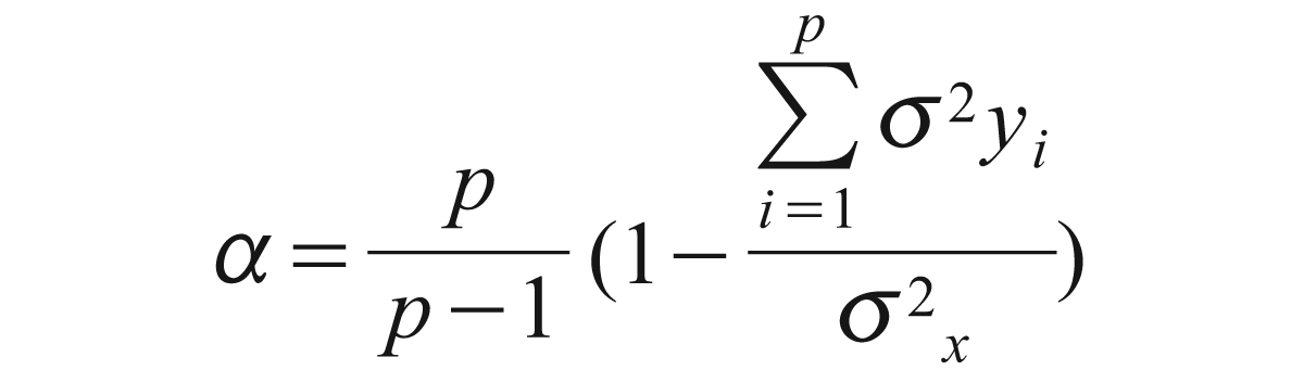
where p is the number of items, $σ_{x}^{2}$ is the variance of the observed total test scores, and $σ_{y_{i}}^{2}$ is the variance of the ith item. The Cronbach’s alpha ranges from 0 to 1, with higher values for greater internal consistency and vice versa. As a rule of thumb, if the Cronbach’s alpha value if less than 0.69 we conclude a poor consistency between the items and alpha between 0.70 and 0.80 is considered a fair amount of consistency.

In Appendix A, the reader will find the R code and the R output for computing Cronbach’s alpha. The three major constructs taken into consideration here are, success, possession and happiness. For each of the constructs, Cronbach’s alpha is calculated. The items that have shown alpha value in the permissible range for consistency were retained and the others discarded. Finally we had arrived at a multidimensional instrument where the individual items were all consistent with the constructs. From the data set under study the Cronbach’s alpha value is 0.733 which is above the threshold value and hence the items used in the instrument can be considered reliable.

As an alternative estimate of reliability we can use the Guttman’s reliability measure given as follows. Out of the six measures, the third is the same as Cronbach’s alpha measure computed above.

Interested readers may refer to Appendix A for the code as well as the output from R for calculating the measures of reliability.

Methodology

In the recent years, the analysis of polytomous manifest variables are handled by the ‘latent trait model’ (ltm) using the graded response theory (grm). The graded response model is a type of polytomous IRT specifically designed for ordinal manifest variables. This model was first discussed by Samejima (1969) and it is mainly used in cases where the assumption of ordinal levels of response options is plausible. The grm postulates that the probability that the kth response for the ith item is expressed as

P (X_{i m} = k | Z_{m}) = g (η_{i k}) - g (η_{i k + 1})

where

η_{i k} = α_{i} (Z_{m} - β_{i k})

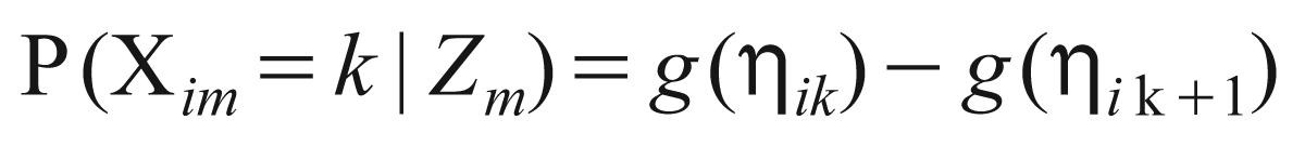
where X_im is the ordinal manifest variable with k possible response categories, Z_m is the standing of the mth subject in the latent trait continuum, α_i denotes the discrimination parameter, and β_ik’s are the extremity parameters with β_i₁ ……… β_ik......... β_{ik –}₁ and β_iki = 3. The interrelation of the discrimination parameter α_i remains the same as in case of dichotomous data; it represents the difficulty in correctly answering the ith item in the questionnaire. In grm, the β_ik’s represent the cut-off points in the cumulative probabilities scale and thus their interpretation is not direct. The Latent trait model fits the grm using the logit link function.

The model is defined as follows:

\log (\frac{y_{i k}}{1 - y_{i k}}) = β_{i} z - β_{i k}

where y_ik denotes the cumulative probability of a response in category ith or lower to the ith item given the latent ability.

If the ‘constrained’ = TRUE then β_i = β for all i.

If IRT.param = TRUE then the parameter estimates are reported under usual IRT parameterization that is

\log (\frac{y_{i k}}{1 - y_{i k}}) = β_{i} z - β_{i k}^{*}

where

β_{i k}^{*} = \frac{β_{i k}}{β i}

For the study that we wish to carry out data were collected using a questionnaire that contained different items for several constructs. We wished to study the attitude and values of the Indian population. A copy of the questionnaire can be found in the Appendix. The three constructs that we have looked at are (i) success, (ii) possession centrality, and (iii) happiness. For each of these constructs there were several items and the data frame contains the responses of 174 individuals to these items. There were six items under the construct happiness, seven for possession centrality and five for happiness. In the previous section, we have seen how we can carry out a test of the internal consistency reliability of our instrument. And to that end we had removed some of the items and the analysis is carried out on the remaining.

We first implement the rcor.test() which is based on the correlation function, cor() of package stats, and it provides us with two options for nonparametric correlation coefficients, namely Kendall’s τ and Spearman’s ρ.

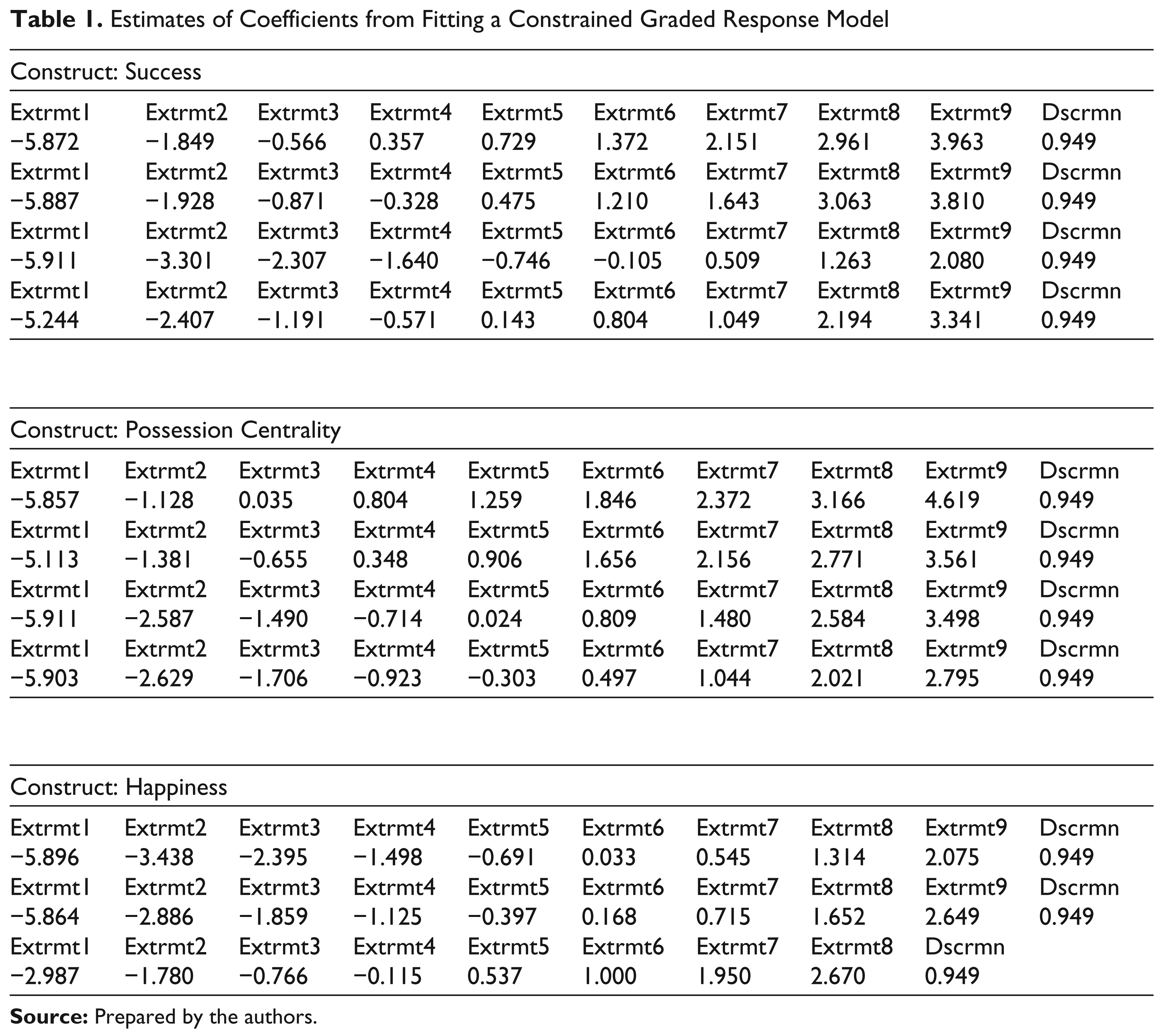
Initially, we fit the constrained graded response model; this model assumes that the discrimination parameter β₁ = β, that is, equal across items. This model can be considered to be equivalent to the Rasch model. The R code for fitting a constrained grm() is provided in the Appendix B. The output we obtain from fitting the grm() model is as follows. The output contains the estimates of the coefficients. In case we wish to test the significance of these coefficients, we can use the Hessian = TRUE option in the call to grm() to obtain the standard error of the estimates and the corresponding p-values.

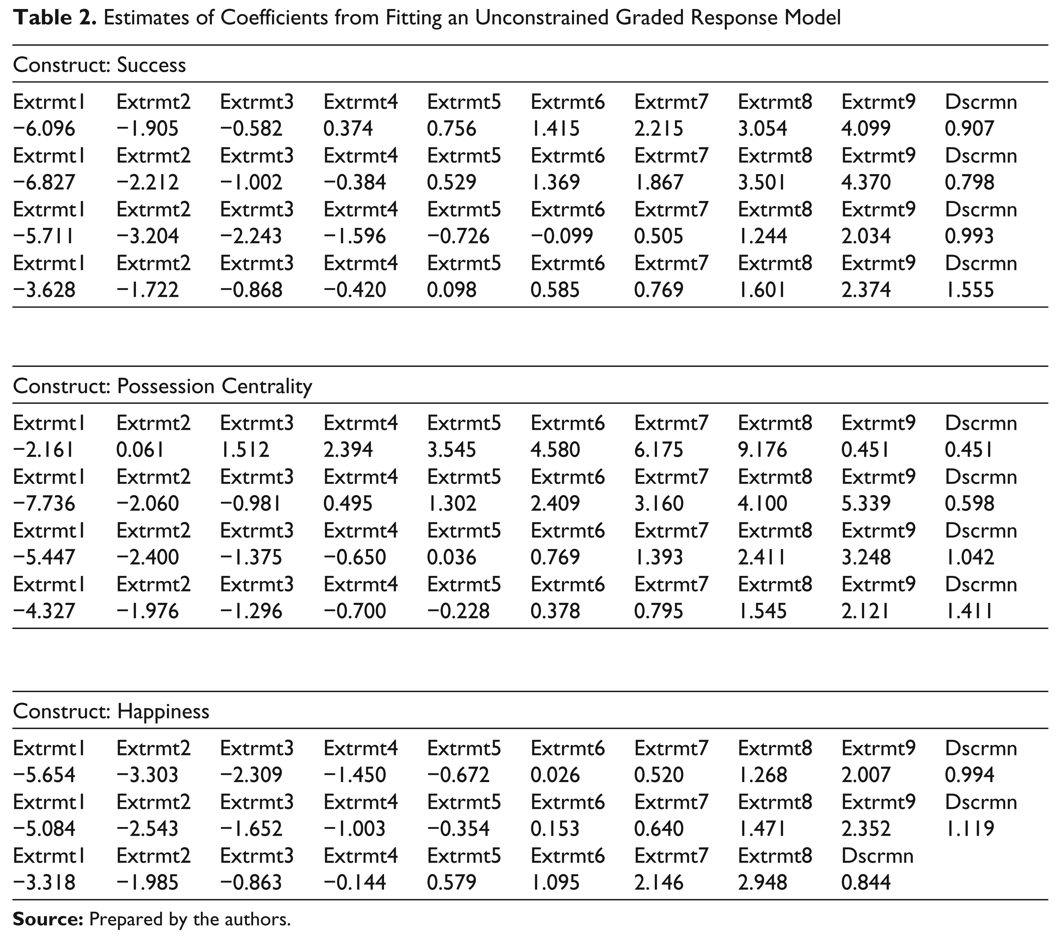
The fit of the grm() model can be checked by the use of margins() method for the grm class. A two-way as well as a three-way margin can be obtained using R. Rather than looking at the whole set of response patterns, margins() help us look at two-by-two contingency tables that contain items at a time. Then the observed and expected correlations for two-way margins are compared to test the fit of the model. For ordinal variates, the comparison is made using the so-called chi-square residuals. A similar technique is followed in case of three-way margins. The only difference is that in three-way margins we take a combination of three items at a time. The check on the fit of the model does not give us the evidence of the overall fit of the model itself. To that end we fit the unconstrained version of the grm to the data. In case of unconstrained grm model, the discrimination parameter is assumed to be different for each respondent. After the fitting of the unconstrained grm, the anova() function gives us the likelihood ratio test p-value that indicates the unconstrained grm is much preferred to the constrained grm for the data.

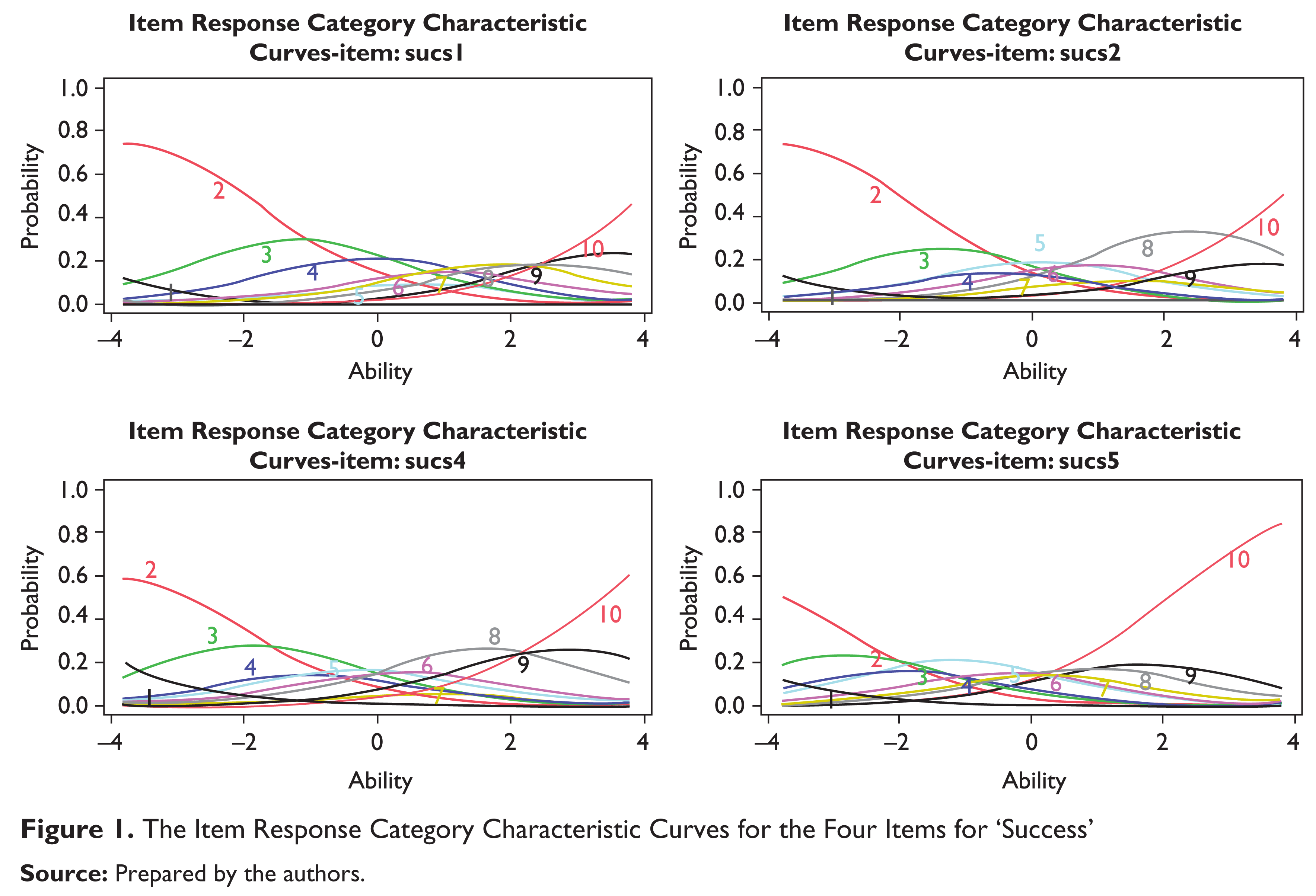
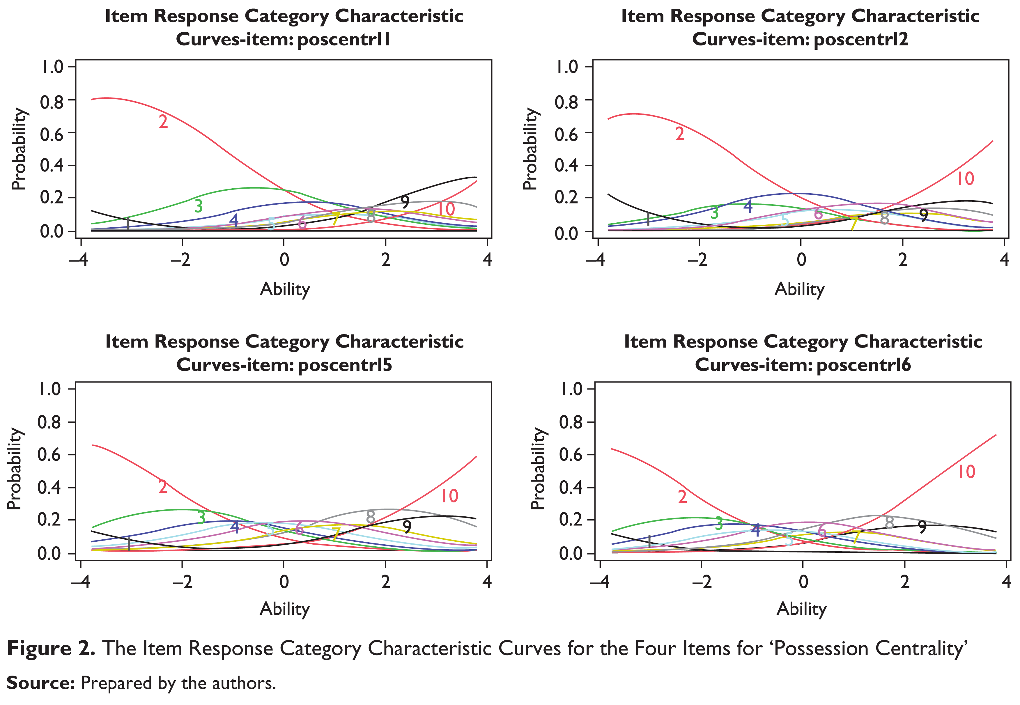
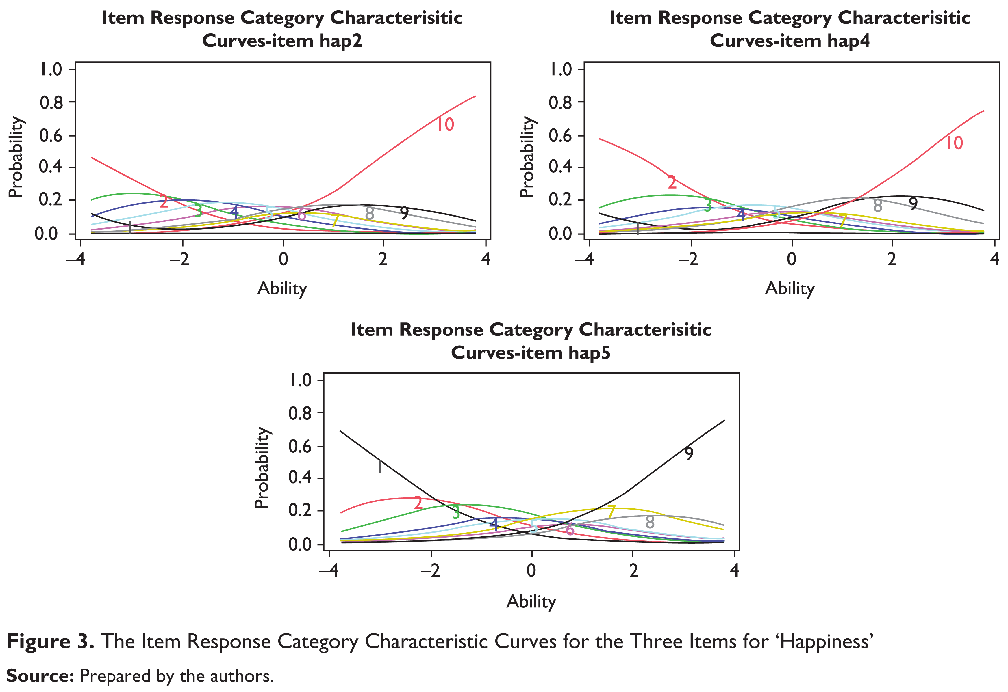
The fitted unconstrained grm can be illustrated by the following figures; the R code used to produce these figures are provided in the Appendix.

Results

In this multidimensional study with polytomous response we have seen the use of a number of items under each of the three latent traits for life satisfaction study, namely ‘Success’, ‘Possession Centrality’ and ‘Happiness’ (Figures 1, 2 & 3). Each of these items has its own response category characteristic curve. If we look at the item response characteristic curves, each one depicts the likelihood or probability of checking that particular response to an item on a scale of 10 as a function of the respondents’ score on the underlying latent trait variable. To be precise, in each of the plots above the curves, each possible response on a 10-point scale has been shown. The reader might notice that each of the curves have their corresponding response value, either 1, 2, 3 so on are depicted next to them. In the plots the term ‘ability’ should be looked upon as the latent trait or latent life satisfaction; ‘ability’ here can be interpreted as the ability to feel happy or successful in their present circumstances. For instance, let us take a look at the example of the first item in the questionnaire ‘sucs1’. The item here asked ‘whether I admire people who own expensive homes, cars, and clothes’. If we wish to check from the curves whether this is a ‘good’ item or not for the latent trait ‘Success’, we immediately see that if we draw our perpendicular at zero and observe that an average respondent is only slightly more likely to assign a ‘3’ or a ‘4’ with some probability that they would assign to anything below ‘3’ or above ‘4’. Had these curves been more peaked and with less overlap than there would have been less ambiguity concerning what values of the latent trait are associated with each category of the rating scale. Each curve for each of the items expresses the probability of selecting the single response alternative as a function of ability. The responses are graded from 1 to 10, where 10 denotes the highest level of response. As we can easily notice, the curve associated with alternative 10 has a monotonic increasing trend meaning that the probability of selecting the option increases as ability increases. On the contrary, the alternative 1 has a monotonic decreasing trend, meaning that the probability of the item approaches zero as ability increases. The intermediate response alternatives 4, 5 and 6 have a non-monotonic trend, increasing for low and intermediate ability levels and decreasing on the rest of the domain. In fact, as the ‘ability’ increases, respondents are more likely to choose a response closer to the higher alternatives like 7, 8 and so on instead of selecting one from the lower spectrum. On the contrary, very ‘successful’ respondents are more likely to answer the item with a high alternative with confidence. From the item characteristic curves for each of the items on the latent traits ‘Success’, ‘Possession’ and ‘Happiness’ opinions tend to follow a predictable path.

Figure 1.

Source: Prepared by the authors.

Figure 2.

Source: Prepared by the authors.

Figure 3.

Source: Prepared by the authors.

Although, we usually take the time to examine the item response characteristic curves, an easier way to do it is by studying the parameter estimates in the graded response model that we have used. In the R output, the columns that are labeled with ‘Extrmt’ are the extremity parameters, the cut points that separate the categories as shown in the bottom row (e.g., 1 vs. 2–10). The first column, Extrmt1, separates the bottom-box from the top-nine categories (1 vs. 2–10). Subsequently the other columns labeled with ‘Extrmt2’ onwards have similar interpretations.

Table 1.

Estimates of Coefficients from Fitting a Constrained Graded Response Model

Construct: Success
Extrmt1	Extrmt2	Extrmt3	Extrmt4	Extrmt5	Extrmt6	Extrmt7	Extrmt8	Extrmt9	Dscrmn
−5.872	−1.849	−0.566	0.357	0.729	1.372	2.151	2.961	3.963	0.949
Extrmt1	Extrmt2	Extrmt3	Extrmt4	Extrmt5	Extrmt6	Extrmt7	Extrmt8	Extrmt9	Dscrmn
−5.887	−1.928	−0.871	−0.328	0.475	1.210	1.643	3.063	3.810	0.949
Extrmt1	Extrmt2	Extrmt3	Extrmt4	Extrmt5	Extrmt6	Extrmt7	Extrmt8	Extrmt9	Dscrmn
−5.911	−3.301	−2.307	−1.640	−0.746	−0.105	0.509	1.263	2.080	0.949
Extrmt1	Extrmt2	Extrmt3	Extrmt4	Extrmt5	Extrmt6	Extrmt7	Extrmt8	Extrmt9	Dscrmn
−5.244	−2.407	−1.191	−0.571	0.143	0.804	1.049	2.194	3.341	0.949

Construct: Possession Centrality
Extrmt1	Extrmt2	Extrmt3	Extrmt4	Extrmt5	Extrmt6	Extrmt7	Extrmt8	Extrmt9	Dscrmn
−5.857	−1.128	0.035	0.804	1.259	1.846	2.372	3.166	4.619	0.949
Extrmt1	Extrmt2	Extrmt3	Extrmt4	Extrmt5	Extrmt6	Extrmt7	Extrmt8	Extrmt9	Dscrmn
−5.113	−1.381	−0.655	0.348	0.906	1.656	2.156	2.771	3.561	0.949
Extrmt1	Extrmt2	Extrmt3	Extrmt4	Extrmt5	Extrmt6	Extrmt7	Extrmt8	Extrmt9	Dscrmn
−5.911	−2.587	−1.490	−0.714	0.024	0.809	1.480	2.584	3.498	0.949
Extrmt1	Extrmt2	Extrmt3	Extrmt4	Extrmt5	Extrmt6	Extrmt7	Extrmt8	Extrmt9	Dscrmn
−5.903	−2.629	−1.706	−0.923	−0.303	0.497	1.044	2.021	2.795	0.949

Construct: Happiness
Extrmt1	Extrmt2	Extrmt3	Extrmt4	Extrmt5	Extrmt6	Extrmt7	Extrmt8	Extrmt9	Dscrmn
−5.896	−3.438	−2.395	−1.498	−0.691	0.033	0.545	1.314	2.075	0.949
Extrmt1	Extrmt2	Extrmt3	Extrmt4	Extrmt5	Extrmt6	Extrmt7	Extrmt8	Extrmt9	Dscrmn
−5.864	−2.886	−1.859	−1.125	−0.397	0.168	0.715	1.652	2.649	0.949
Extrmt1	Extrmt2	Extrmt3	Extrmt4	Extrmt5	Extrmt6	Extrmt7	Extrmt8	Dscrmn
−2.987	−1.780	−0.766	−0.115	0.537	1.000	1.950	2.670	0.949

Source: Prepared by the authors.

Table 2.

Estimates of Coefficients from Fitting an Unconstrained Graded Response Model

Construct: Success
Extrmt1	Extrmt2	Extrmt3	Extrmt4	Extrmt5	Extrmt6	Extrmt7	Extrmt8	Extrmt9	Dscrmn
−6.096	−1.905	−0.582	0.374	0.756	1.415	2.215	3.054	4.099	0.907
Extrmt1	Extrmt2	Extrmt3	Extrmt4	Extrmt5	Extrmt6	Extrmt7	Extrmt8	Extrmt9	Dscrmn
−6.827	−2.212	−1.002	−0.384	0.529	1.369	1.867	3.501	4.370	0.798
Extrmt1	Extrmt2	Extrmt3	Extrmt4	Extrmt5	Extrmt6	Extrmt7	Extrmt8	Extrmt9	Dscrmn
−5.711	−3.204	−2.243	−1.596	−0.726	−0.099	0.505	1.244	2.034	0.993
Extrmt1	Extrmt2	Extrmt3	Extrmt4	Extrmt5	Extrmt6	Extrmt7	Extrmt8	Extrmt9	Dscrmn
−3.628	−1.722	−0.868	−0.420	0.098	0.585	0.769	1.601	2.374	1.555

Construct: Possession Centrality
Extrmt1	Extrmt2	Extrmt3	Extrmt4	Extrmt5	Extrmt6	Extrmt7	Extrmt8	Extrmt9	Dscrmn
−2.161	0.061	1.512	2.394	3.545	4.580	6.175	9.176	0.451	0.451
Extrmt1	Extrmt2	Extrmt3	Extrmt4	Extrmt5	Extrmt6	Extrmt7	Extrmt8	Extrmt9	Dscrmn
−7.736	−2.060	−0.981	0.495	1.302	2.409	3.160	4.100	5.339	0.598
Extrmt1	Extrmt2	Extrmt3	Extrmt4	Extrmt5	Extrmt6	Extrmt7	Extrmt8	Extrmt9	Dscrmn
−5.447	−2.400	−1.375	−0.650	0.036	0.769	1.393	2.411	3.248	1.042
Extrmt1	Extrmt2	Extrmt3	Extrmt4	Extrmt5	Extrmt6	Extrmt7	Extrmt8	Extrmt9	Dscrmn
−4.327	−1.976	−1.296	−0.700	−0.228	0.378	0.795	1.545	2.121	1.411

Construct: Happiness
Extrmt1	Extrmt2	Extrmt3	Extrmt4	Extrmt5	Extrmt6	Extrmt7	Extrmt8	Extrmt9	Dscrmn
−5.654	−3.303	−2.309	−1.450	−0.672	0.026	0.520	1.268	2.007	0.994
Extrmt1	Extrmt2	Extrmt3	Extrmt4	Extrmt5	Extrmt6	Extrmt7	Extrmt8	Extrmt9	Dscrmn
−5.084	−2.543	−1.652	−1.003	−0.354	0.153	0.640	1.471	2.352	1.119
Extrmt1	Extrmt2	Extrmt3	Extrmt4	Extrmt5	Extrmt6	Extrmt7	Extrmt8	Dscrmn
−3.318	−1.985	−0.863	−0.144	0.579	1.095	2.146	2.948	0.844

Source: Prepared by the authors.

Thus, in this article as a measurement task, we have an estimate of each individual’s latent position on an underlying continuum defined as what determines the item responses. Along the way, we discover which items require more of the latent trait in order to achieve a favourable response.

Summary of Results

From the analysis of the scale data on life satisfaction using IRT, we can conclude that as the ‘ability’ to be happy or satisfied with their life increases so does the confidence in answering the polytomous items with a higher response. Also due to the use of the IRT as opposed to the much used Likert scale, we could draw item characteristic curve for individual items and the difficulty of each item could be incorporated in the scaling items.

Conclusions and Recommendations

This is a relatively new method of addressing issues related to analyzing psychometric data in marketing where use of scales are common. Although our results largely mirror those of classical psychometry, we need to examine these issues further. To conclude, this article does not question the utility of the classical methods but we explore an alternative distribution-free method which may enhance the explanatory power of the existing methods.

Footnotes

Acknowledgements

The authors are grateful to the anonymous referees of the journal for their extremely useful suggestions to improve the quality of the article.

Appendix

References

Baker

F.B.

(2001). The basics of item response theory. University of Wisconsin: ERIC Clearinghouse on Assessment and Evaluation.

Birnbaum

(1968). Some latent trait models and their use in inferring an examinee’s ability. In Lord

F.M.

& Novick

M.R.

(Eds), Statistical theories of mental test scores (pp. 397–479), Reading, MA: Addison-Wesley.

Ghosh

, & Srivastava

B.K.

(2014). Construction of a reliable and valid scale for measuring organizational culture. Global Business Review, 15(3), 583–596.

Hambleton

K.R.

, & Russell

J.N.

(1993). Comparison of classical test theory and item response theory and their application to test development. Philadelphia, USA: University of Massachusetts, Instructional Topics in Educational Measurement.

Lord

F.M.

, Novick

M.R.

, & Birnbaum

(1968). Statistical theories of mental test scores. Oxford, England: Addison-Wesley.

Richins

M.L.

, & Dawson

(1992). Materialism as a consumer value: Measure development and validation. Journal of Consumer Research, 19(December), 303–316.

Rizopoulos

(2006). Itm: An R package for latent variable modeling and item response theory analyses. Journal of Statistical Software, 17(5), 1–25.

Samejima

(1969). Estimation of latent ability using a response pattern of graded scores. Psychometrica Monograph Supplement No. 17, 34.