Finance–Growth–Energy Nexus and the Role of Agriculture and Modern Sectors: Evidence from ARDL Bounds Test Approach to Cointegration in Pakistan

Abstract

This article explores the relationship between financial development and energy consumption by incorporating economic growth, agriculture and modern sectors in Pakistan over the period 1972–2011. The autoregressive distributive lag (ARDL) bounds testing approach to cointegration, assuming structural breaks, confirms cointegration. Innovation accounting approach, used to examine the direction of causality, shows that economic growth causes energy demand. We also fine bidirectional causality between financial development and energy consumption, and between modern sector growth and energy consumption. Energy consumption Granger causes agriculture growth. The results offer valuable insights for policymakers in crafting appropriate energy policy for Pakistan.

Keywords

Energy consumption economic growth financial development Pakistan

Introduction

Energy economics in general, and the link between energy consumption and economic growth in particular, has drawn considerable attention from the academicians and policymakers in recent times. The topic is important due to the derived demand nature of energy. Energy drives the wheels of an economy. The significant spurt in global energy demand can be ascribed to two main sources: (i) rapid economic growth in the emerging nations and (ii) maintenance of the relatively high living standards in the developed nations. The intuitive idea that raising growth rate of per capita gross domestic product (GDP) requires more energy has been confirmed by the pioneering study of Kraft and Kraft (1978). For the US, they found unidirectional causality from gross national product (GNP) to energy use during the period 1947–1974.

The sizeable literature on the output–energy or output–pollution nexus portrays only a partial picture. For example, Lee and Chang (2008) included capital stock and labour to examine energy demand for some Asian nations. They found a positive link between economic growth and energy demand which gets stronger as more relevant variables are included. Apergis and Payne (2009a, 2009b, 2010) and Wolde-Rufael (2009) argue that rise in energy demand in emerging economies is closely linked to the growth of income. As population grows, pressure on limited rural resources forces people to move to urban areas which adds to the energy demand. For a sustained economic growth, the increased energy demand over a long period must be met from new sources, or by developing cost-effective alternative sources. Using both bivariate and multivariate models for New Zealand, Bartleet and Gounder (2010) found that causality runs from real GDP to energy use. They also note that capital stock plays an important role in determining the direction of causality.

The objective of this article is to explore a long-run relationship among economic growth, energy consumption, financial development, contribution of agriculture and modern sectors in Pakistan by implementing the autoregressive distributive lag (ARDL) bounds testing approach to cointegration. We use annual data from 1972 to 2011. The study period spanning four decades is hallmarked by major changes in the local and global landscape which can potentially cause structural break in the series. Not factoring such feature can lead to model misspecification and produce low power of unit root test (see Perron, 1989). To finesse this, we apply the Zivot–Andrews (ZA) (1992) unit root test which accommodates a single unknown structural break. The motivation behind undertaking the study on Pakistan, a nation of 175 million in the Indian subcontinent, is primarily driven by the inquisitiveness to examine the energy–growth nexus in light of the ongoing structural transformation. While we consider a set of relevant variables, research shows that the latter can be an important driver of economic growth. The article contributes to the literature in several distinct ways. (i) Pakistan’s economy is characterized by a combination of a sizeable agricultural and a modest manufacturing sector. The value added by agricultural and manufacturing sectors separately helps to capture elements of ongoing structural transformation in Pakistan. This is the first comprehensive study that examines the dynamic interactions among economic growth, financial development, energy consumption along with some measure of structural transformation. (ii) From methodological perspective, we apply the ARDL approach which is well suited to a small sample. We also apply a unit root test which is capable of detecting structural break in the series. (iii) The inclusion of financial development in the model appears justified due to Pakistan’s decision to liberalize the financial sector. (iv) The innovative accounting technique (IAA) used to examine the direction of causality has some advantages over the traditional Granger approach. The latter test does not determine the relative strength of the causality beyond the selected time span (Shan, 2005); nor does it show the extent of feedback from one variable to the other. The IAA avoids these shortcomings. The authors are not aware of a similar study for Pakistan which makes it a contribution to the literature. The findings should help policymakers to better understand the interaction among the series in crafting a sustainable policy.

Literature Review

In this section, we review the extant literature along the three main strands: economic growth and energy consumption; economic growth and financial development; and financial development and energy consumption.

Economic Growth and Energy Consumption

The literature on energy–growth nexus is expansive. For example, Yu and Choi (1985), Stern (1993, 2000), Yang (2000), Alam and Butt (2002), Oh and Lee (2004), Yoo (2006), Lee and Chang (2008) and Beaudreau (2005, 2010), among others, find energy to be important for economic growth. Others consider energy consumption, GDP and energy price as the variables of interest. Several studies have examined the nexus of energy consumption, energy prices and economic growth and there are others that ignored the role of urbanization, trade, industrialization and financial development, although they are relevant to energy demand (see Mishra, Smyth & Sharma, 2009; Sadorsky, 2011; Shahbaz & Lean, 2012; Shahbaz et al., 2013).

As for Pakistan, only a few studies have examined the causality between energy consumption and economic growth. Aqeel and Butt (2001), Alam and Butt (2002), Siddiqui (2004), Khan and Qayyum (2007), Qazi and Riaz (2008) and Shahbaz et al. (2012a) used different indicators of energy use to examine the causality relationship between energy consumption and economic growth. The studies failed to find a consistent pattern on the direction of causality which might be due to the differences in methodology, use of indicators of energy consumption and possibly the time span used. Also exclusion of some relevant variables might have led to model misspecification.

Financial Development and Economic Growth

The link between financial development and economic growth has gained prominence with globalization taking the centre stage. A developed financial system can help to achieve efficiency in the financial transactions, promote innovations, lower information cost, help adoption of advanced technology and ensure efficient allocation of investment funds (Abu-Bader & Abu-Qarn, 2008; Bairer, Dwyer & Tamura, 2004; Greenwood & Jovanovich, 1990; Levine, 1997; Shahbaz et al., 2010a; Townsend, 1979). Patrick (1966) noted that ‘demand–following’ relationship implies that real economic activity Granger causes financial development through demand for financial services. This happens as an economy grows and the need for financial sector development becomes intense. Robinson (1952), Lucas (1988) and Stern (1989) suggest that financial development follows economic growth. The former promoted economic growth by raising savings and enhancing capital. Broadly, financial markets help to raise internal and external resources and promote economic growth (Bencivenga & Smith, 1991; Greenwood & Jovanovich, 1990).

Ibrahim (2007) found that financial development stimulates economic growth in Malaysia; so did Shahbaz (2009) for Pakistan. A sound financial market reduces financial instability¹ and thereby aids economic growth. Using investment as a variable, Odhiambo (2010) found that financial development promotes economic growth in South Africa where the former follows the latter and is closely related to foreign capital inflows. Financial development stimulates equity markets, allows easy access to financial capital, facilitates inflow of foreign direct investment (FDI) and lowers financial risk. Broadly, financial development improves monetary transmission mechanism, boosts savings and investment and promotes economic growth. Fung (2009) found that the growth augmenting effect of financial development is facilitated by productivity boost (see Beakert & Harvey, 2000; Beakert et al., 2001, 2002, 2005). Shahbaz (2012) found that trade openness helps finance-led growth in Pakistan.

Financial Development and Energy Consumption

Financial development affects energy consumption through consumption and production channels. Financial development can affect real variables, that is, investment and real interest rate (Zicchino, 2006). From production side, it lowers borrowing cost, enhances investment (local and foreign), boosts output and generates employment. Low interest rate helps purchase of consumer durables (Mankiw & Scarth, 2008; Sadorsky, 2010). All these add to energy use. Karanfil (2009) argued that causality analysis between energy and economic growth needs to go beyond a simple bivariate framework. He recommended using stock market capitalization, liquid liabilities and domestic credit to the private sector as share of GDP as potential explanatory variables. He suggested that exchange rates and interest rates may influence energy demand through the price channel.

Following the suggestion by Karanfil (2009), Dan and Lijun (2009) examined the impact of financial development on primary energy consumption in Guangdong (China). They found causality from energy consumption to financial development. Sadorsky (2010) applied different indicators of financial development to 22 emerging economies (1990–2006).² He found that the impact of financial development on energy demand is positive but small. Shahbaz and Lean (2012a) found that financial development promotes economic growth and increases energy demand in Tunisia. They also report feedback effect between financial development and energy use. The same is true for industrialization and energy consumption. Chtioui (2012) reported that the effect of financial development and economic growth on energy consumption is positive. Financial development Granger causes energy consumption, but feedback effect exists between economic growth and energy consumption. Xu (2012) applied various indicators of financial development to Chinese provincial data from 1999 to 2009 and found a positive link between the two series. For Iran, Mehrara and Musai (2012) found that economic growth, financial development and energy consumption are cointegrated, and that the impact of energy consumption on economic growth is negative, while the reverse is true of capital, oil revenues and financial development. Tang and Tan (2012) reported the bidirectional causality between financial development and energy consumption in short and long runs. Islam et al. (2013) found that financial development, economic growth and population led to the rise in energy demand in Malaysia. They found the feedback effect between financial development and energy consumption in the long run. Coban and Topeu (2013) found a positive and significant impact of financial development on energy consumption in ‘old members of EU’. However, for the new members, the link between financial development and energy consumption is sensitive to the choice of an indicator. They found an inverted-U relationship between the two series in the models that use stock market capitalization as the indicator of financial development.

Model Construction and Research Methods

The annual data from 1972 to 2011 relating to the variables is taken from the World Development Indicators (WDI-CD, 2012). Each series is measured in per capita terms. Energy consumption, denoted by E_t, is measured by energy consumed (kilowatt of oil equivalent). Financial development, denoted by F_t, is measured by the real stock market capitalization of the listed companies in the equity market.³ Growth in real GDP, Y_t, measures economic growth. Value added in the agriculture and modern sectors (measured by value added of industrial and services sectors to GDP) is denoted by A_t and M_t respectively. The following relation is posited. For estimations, the empirical model is specified in following equation.

E_{t} = f (F_{t}, Y_{t}, A_{t}, M_{t})

(1)

We specify the estimable equation⁴ in log-linear form as follows:

\ln E_{t} = δ_{o} + δ_{F} \ln F_{t} + δ_{Y} \ln Y_{t} + δ_{A} \ln A_{t} + δ_{M} \ln M_{t} + μ_{t}

(2)

A high value of stock market capitalization shows a developed and efficient equity market where funds are channelled to high-return projects (level effect), and is pro-economic growth (Minier, 2009; Sadorsky, 2010). Developed financial markets enhance investor confidence, attract FDI and boost economic growth (Sadorsky, 2010). These are further pushed by the efficiency effect which ensures that stock market channels liquidity, diversifies assets and secures finance for the projects; so δ_F > 0. Growing economies consume more energy⁵; so δ_Y > 0. Agriculture uses traditional technology and is hence less efficient. So, we expect δ_A > 0. Modern sector growth by contrast uses advanced and energy-efficient technology, so that δ_M < 0.

Ng–Perron (2001) developed generalized least square (GLS)-based test statistics to test the stationarity of a series. The critical values of the tests are based on Phillips–Perron’s (1988) Z_α and Z_t statistics, Bhargava’s (1986) R₁ statistics and Elliot, Rothenberg and Stock’s (1996) critical values. The following annotations are used:

k = \sum_{t = 2}^{T} {(y_{t - 1}^{d})}^{2} / T ​^{2}

(3)

The de-trended GLS tailored statistics are given by:

M Z_{a}^{d} = (T^{- 1} {(y_{T}^{d})}^{2} - f_{o}) / (2 k)

M Z_{t}^{d} = M Z_{a} \times M S B

M S B^{d} = {(k / f_{o})}^{1 / 2}

M P_{T}^{d} = (δ^{2} k - δ T^{- 1}) {(y^{d} T)}^{2} / f_{o} i f x_{t} = 1 a n d M P^{d} T (δ^{2} k + (1 - δ) T^{- 1} {(y^{d} T)}^{2} / f_{o} i f x_{t} = (1, t)

(4)

where δ = –7, if x_t = 1 and δ = –13.5, if x_t = (1, t)

As noted, we apply unit roots test appropriate for structural break. Zivot–Andrews (1992) and Perron and Volgelsang (1992) unit root tests are appropriate when the series contains one structural break. Zivot–Andrews approach considers three possible alternatives: (i) a one-time change at the levels; (ii) a one-time change in the slope; and (iii) a one-time change both in intercept and in trend. Each of the three scenarios can be modelled as follows:

Δ x_{t} = a + a x_{t - 1} + b t + c D U_{t} + \sum_{j = 1}^{k} d_{j} Δ x_{t - j} + μ_{t}

(5)

Δ x_{t} = b + b x_{t - 1} + c t + b D T_{t} + \sum_{j = 1}^{k} d_{j} Δ x_{t - j} + μ_{t}

(6)

Δ x_{t} = c + c x_{t - 1} + c t + d D U_{t} + d D T_{t} + \sum_{j = 1}^{k} d_{j} Δ x_{t - j} + μ_{t}

(7)

where the dummy variable is indicated by DU_t showing that mean shift occurred at each point with time break, while trend shift variables are shown by DT_t. So,

D U_{t} = {\frac{1... i f t > T B}{0... i f t < T B} a n d D U_{t} = {\frac{t - T B ... i f t > T B}{0... i f t < T B}

The null hypothesis of unit roots break date is c = 0 which indicates that the series is not stationary with a drift not having information about structural break point, while c < 0 hypothesis implies that the variable is found to be trend-stationary with one unknown time break. Zivot–Andrews unit root test considers all points as potential break points and estimates them successively and finally picks the break when $\hat{c} (= c - 1) = 1$ from a region where the end points of sample period are excluded.

The ARDL bounds testing approach is used to explore the long-run equilibrium relation in the presence of structural break among series energy consumption (E_t), financial development (F_t), economic growth (Y_t), agriculture growth (A_t) and growth in modern sector (M_t). The bounds testing approach applies irrespective of the order of integration of the regressors I(0) or I(1), although an I(2) can cause problem (Ouattara, 2004). A dynamic unrestricted error-correction model (UECM) is derived from the ARDL by using a simple linear transformation. The error-correction model (ECM) combines short-run dynamics with long-run equilibrium without losing long-run information. The ARDL approach involves estimating the following UECM:

Δ y = α_{o} + λ_{D} D + λ_{2} y_{t - 1} + λ_{3} z_{t - 1} + λ_{4} x_{t - 1} + \sum_{i = 1}^{p} γ_{i} Δ y_{t - 1} + \sum_{j = 0}^{p} α_{i} Δ x_{t - j} + \sum_{s = 0}^{p} w_{s} Δ z_{t - s} + ε_{i}

(8)

where α_o is a drift component and ε_i a white noise process. The ARDL approach estimates (p + 1)^k number of regressions to obtain optimal lag length for each series. Here ‘p’ is the maximum number of lags used and ‘k’ the number of variables in equation (8). The optimal lag structure of the first difference regression is selected by using both the Akaike information (AIC) and the Schwarz Bayesian (SBC) criteria. The lagged terms help to induce white noise properly to the error term. Based on Pesaran, Shin and Smith’s (2001) study, we used the bounds test for a long-run relationship and the F-test for joint significance of the coefficients of the lagged variables in equation (8). The long-run relation holds if the null hypothesis of no cointegration H_o: λ₂ = λ₃ = λ₄ = 0 is rejected in favour of the alternative H_a: λ₂ ! λ₃ ! λ₄ ! 0. Two asymptotic critical bounds are used when the independent variables are I(d) (0 ≤ d ≤ 1).

If the F-statistic exceeds the upper critical bound (UCB), we conclude in favour of a long-run relationship, regardless of the order of integration, but if it is below the lower critical bound (LCB), the null hypothesis of no cointegration is sustained. The test is inconclusive if the F-statistic lies between the two bounds. When the order of integration for the explanatory variables is I(1), the decision is made based on the UCB, and if it is I(0), the decision is based on the LCB. If cointegration exists, the conditional long-run model is derived from the reduced form of equation (8) when the series in first difference are jointly equal to zero, that is, $Δ x = Δ y = Δ z = 0$ . Thus,

y_{t} = \partial_{o} + \partial_{2} x_{t} + \partial_{3} z_{t} + μ_{i}

(9)

where $\partial_{o} = - λ_{1} / λ_{2}; \partial_{2} = - λ_{3} / λ_{2}; \partial_{3} = - λ_{4} / λ_{2};$ and v_t is the random error. The long-run coefficients are estimated using ordinary least square (OLS) from equation (9). If a long-run relation is found, an error correction representation exists which is estimated from the following reduced form equation:

Δ y_{t} = \sum_{i = 1}^{p} λ_{i} Δ y_{t - 1} + \sum_{j = 1}^{m} β_{i} Δ x_{t - j} + \sum_{k = 1}^{n} β_{k} Δ z_{t - k} + η E C M_{t - 1} + ε_{i}

(10)

To assess goodness of fit of the ARDL model, we apply the diagnostic and the stability tests. The former is used to check for serial correlation, functional form, heteroskedasticity and normality of the error terms. The stability test employs the cumulative sum (CUSUM) and the CUSUM squared (CUSUMsq).

The IAA involves two steps: (i) decomposing forecast error variance and (ii) generating impulse response function (IRF). The decomposition process splits the proportion of variation in a series into those caused by its own shocks and those coming from others (Enders, 1995) are used to show the strength of the impact. In practice, a system of equation is used to examine the impact of one standard deviation shock to the variable on others and also on the future values of the series sustaining the shock (Shan, 2005). The IRF on the other hand, traces out the time path of the impacts of a series.

For instance, if shock to financial development affects energy consumption significantly but a shock on the latter affects the former minimally, then we have unidirectional causality from the former to the latter. If the energy consumption explains more of forecast error variance of financial development, then energy consumption causes financial development in the Granger sense. The bidirectional causality exists if shocks affect each variable strongly, while minimal impact implies absence of causality between them. As noted, the IRF helps us to trace out the time path of the impacts of shock on variables in the vector autoregression (VAR). For example, financial development is said to cause energy consumption if the IRF triggers strong response of the latter to shocks in the former compared to other series. A VAR system takes the following form:

V_{t} = \sum_{i = 1}^{k} δ_{i} V_{t - 1} + η_{t}

where V_t = (E_t, F_t, Y_t, A_t, M_t), η_t = (η_E, η_F, η_Y, η_A, η_M), δ₁ – δ_k are four-by-four matrices of coefficients and η is a vector of error terms.

Results and Discussion

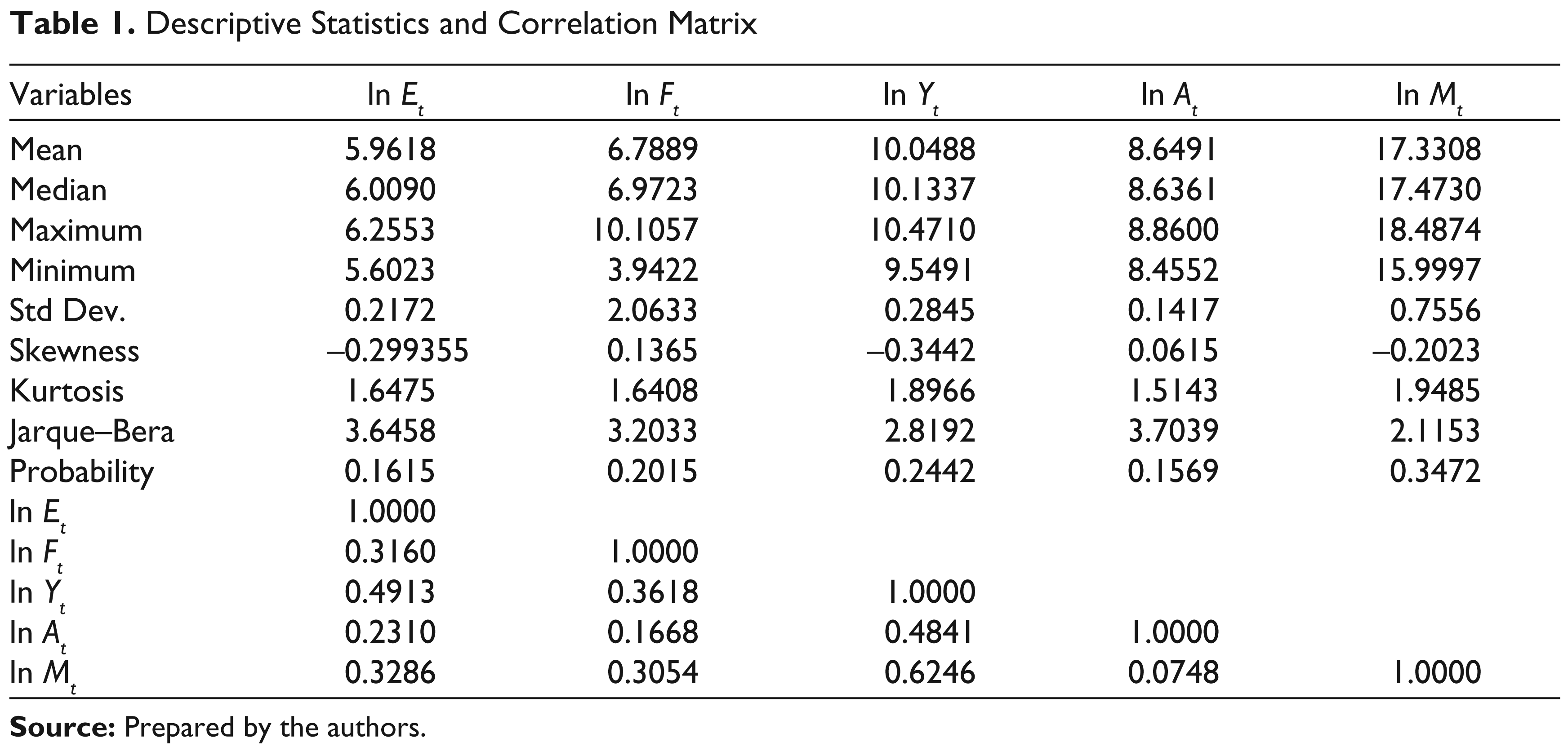
Table 1 reports the descriptive statistics and the correlation matrix. Jarque–Bera test confirms normality of each series. The correlation between each pair of variables is positive.

Table 1.

Descriptive Statistics and Correlation Matrix

Variables	ln E_t	ln F_t	ln Y_t	ln A_t	ln M_t
Mean	5.9618	6.7889	10.0488	8.6491	17.3308
Median	6.0090	6.9723	10.1337	8.6361	17.4730
Maximum	6.2553	10.1057	10.4710	8.8600	18.4874
Minimum	5.6023	3.9422	9.5491	8.4552	15.9997
Std Dev.	0.2172	2.0633	0.2845	0.1417	0.7556
Skewness	–0.299355	0.1365	–0.3442	0.0615	–0.2023
Kurtosis	1.6475	1.6408	1.8966	1.5143	1.9485
Jarque–Bera	3.6458	3.2033	2.8192	3.7039	2.1153
Probability	0.1615	0.2015	0.2442	0.1569	0.3472
ln E_t	1.0000
ln F_t	0.3160	1.0000
ln Y_t	0.4913	0.3618	1.0000
ln A_t	0.2310	0.1668	0.4841	1.0000
ln M_t	0.3286	0.3054	0.6246	0.0748	1.0000

Source: Prepared by the authors.

Given that the standard unit root tests may produce unreliable results in the presence of structural break in the series (Zivot, Andrews, 1992), we complement the Ng–Perron unit root with the ZA (1992) unit root test. The Ng–Perron test results, reported in Table 2, show that all the series are I(1) with intercept and trend. The ZA test results reported in Table 3 also confirm the order of integration as I(1).

We apply the AIC to choose an appropriate lag length because of its better power properties compared to others (Shahbaz & Rahman, 2012). The ARDL F-statistic is sensitive to the lag order. The lag length of the series is given in column 2 of Table 4. Our results of the ARDL bounds testing are also reported in Table 4.

Table 2.

Unit Root Test

Ng–Perron Test at Level
Variables	Mza	MZt	MSB	MPT
ln E_t	–8.6405(2)	–1.9688	0.2278	10.9152
ln F_t	–9.9813(1)	–2.2206	0.2224	9.1893
ln Y_t	–4.1032(1)	–1.3765	0.3354	21.5912
ln A_t	–8.5005(1)	–2.0616	0.2425	10.7199
ln M_t	–12.4070(1)	–2.4334	0.1961	7.6534
Ng–Perron Test at 1st Difference
Dln E_t	–19.0795(2)**	–3.0867	0.1617	4.7873
Dln F_t	–19.3433(3)**	–3.0891	0.1597	4.8365
Dln Y_t	–18.3730(1)**	–3.0309	0.1649	4.9597
Dln A_t	–22.3856(1)*	–3.3403	0.1492	4.1020
Dln M_t	–35.6680(3)*	–4.2085	0.1179	2.6343

Source: Prepared by the authors.

Note: * and ** indicate the significance at the 1% and 5% levels. Lag order is shown in parentheses.

Table 3.

Zivot–Andrews Structural Break Unit Root Test

Variable	At Level		At 1st Difference
Variable	T-Statistic	Time Break	T-statistic	Time Break
ln E_t	–4.027(0)	1987	–6.957(3)*	1979
ln F_t	–3.438 (2)	1992	–6.865(1)*	2003
ln Y_t	–3.405 (1)	1993	–5.752 (2)*	1993
ln A_t	–4.144 (0)	1995	–8.151 (0)*	1997
ln M_t	–3.654 (1)	1993	–5.091 (1)**	1987

Source: Prepared by the authors.

Note: * and ** represent significant at 1%, 5% level of significance. Lag order is shown in parenthesis.

Table 4.

The Results of ARDL Cointegration Test

Bounds Testing to Cointegration				Diagnostic Tests
Estimated Models	Optimal Lag Length	F-statistics	Structural Break	χ ² _NORMAL	χ ² _ARCH	χ ² _RESET
F_E(E/Y, F, A, M)	2, 1, 2, 2, 2	8.113*	1987	1.0810	[1]: 0.0134	[1]: 2.2426
F_Y(Y/E, F, A, M)	2, 2, 2, 2, 1	2.881	1992	0.0736	[2]: 1.1174	[1]: 0.6200
F_F(F/E, Y, A, M)	2, 2, 2, 1, 2	1.192	1993	1.8050	[2]: 0.9063	[1]: 1.0193
F_A(A/E, Y, F, M)	2, 2, 2, 2, 2	9.897*	1995	0.1819	[1]: 0.4543	[1]: 0.0392
F_M(M/E, Y, F, A)	2, 2, 2, 1, 1	6.174**	1993	0.7932	[1]: 1.7448	[1]: 0.2294
Significant Level ^#	Critical Values (T = 41)
Significant Level ^#	Lower Bounds I(0)	Upper Bounds I(1)
1% level	5.893	7.337
5% level	4.133	5.260
10% level	3.373	4.377

Source: Prepared by the authors.

Notes: 1. * and ** denote the significant at 1% and 5% levels, respectively.

2. The optimal lag length is determined by AIC.

3. [ ] is the order of diagnostic tests.

4. ^# Critical values are collected from Narayan (2005).

To test cointegration, we take the critical bounds from Narayan (2005) rather than Pesaran et al. (2001). The latter are suitable in large samples (T = 500 or higher) and can produce downward bias (Narayan & Narayan, 2004) in small samples. Narayan’s (2005) critical bound is more appropriate for sample ranging from T = 30 to T = 80. We find the computed F-statistic to exceed the UCB at 1 per cent and 5 per cent when energy consumption, agriculture and modern sector are the predicted variables. The series energy consumption, agricultural growth and growth in modern sector show structural breaks occurring in 1987, 1995 and 1993, respectively. The severe drought in Pakistan in 1987 may have caused the structural break in energy consumption series. The agriculture growth series was impacted by the rise in cotton prices in 1995. The government policy to promote industrial and services sectors was captured in 1993. The results confirm cointegration among the series from 1972 to 2011 for Pakistan.

Table 5 presents the long-run elasticity of energy consumption with respect to independent variables. Financial development and energy consumption are positively related and significant at 10 per cent level. A 10 per cent increase in financial development (stock market capitalization) is expected to raise the energy demand by 1.486 per cent, ceteris paribus. High stock market capitalization enhances investors’ confidence, stimulates economic growth and thus boosts energy use. Also credit availability makes it easier for consumers to purchase big-ticket durable items, which adds to energy demand. Our findings lend support to those by Sadorsky (2010), Shahbaz and Lean (2012a) and Islam, Shahbaz, Ahmed and Alam (2013). These authors found a higher elasticity than ours which might have been due the difference in measuring financial development.

Results suggest that the effect of economic growth on energy consumption is sizeable. A 1 per cent rise in economic growth increases energy demand by about 0.8769 per cent. (All elasticity measures reported here are on ‘an average’ and ‘ceteris paribus’.) The results are consistent with those found by Aqeel and Butt (2001) and Bowden and Payne (2009) for Pakistan; Bowden and Payne (2009) for USA; Halicioglu (2009) for Turkey; Odhiambo (2009) for Tanzania; Shahbaz and Lean (2012a) for Tunisia; and Islam et al. (2013) for Malaysia. The impact of agriculture growth is positive and statistically significant at the 1 per cent level. A rise by 0.2113 per cent in energy demand is linked to a 1 per cent increase in agriculture growth. These finding are consistent with the findings of Mushtaq, Abbas and Abedullah (2007) who noted that an increase in agricultural value added raises energy demand. The relation between the growth in modern sector and energy consumption is negative and statistically significant at 5 per cent level. It may be noted that modern sector uses energy-efficient technology. A 1 per cent rise in modern sector growth is linked with 0.1216 per cent decline in energy demand. Yildirim, Aslan and Ozturk (2012) found a negative relationship between industrial production and energy consumption in the USA.

The short-run results can be seen in the lower segment of Table 5. The coefficient of financial development shows positive and significant effect on energy consumption. However, short-run coefficient is smaller than the long-run coefficient. Energy consumption increases by 0.014 per cent in response to a 1 per cent rise in the stock market capitalization. A 1 per cent increase in economic growth raises energy consumption by 0.389 per cent. The impacts of agricultural sector growth and modern sector growth are positive and negative, respectively, but not significant in the short run.

Table 5.

Long- and Short-run Analyses

Dependent Variable: ln E_t
Long-run Results
Variable	Coefficient	Std Error	t-Statistic
Constant	–2.6705*	0.7212	–3.7025
ln F_t	0.1486***	0.0781	1.9017
ln Y_t	0.8769*	0.1520	5.7669
ln A_t	0.2113**	0.0794	2.6599
ln M_t	–0.1216**	0.0594	–2.0475
Short-run Results
Variable	Coefficient	Std Error	t-Statistic
Constant	0.0057	0.0038	1.4706
Dln F_t	0.0148***	0.0082	1.7948
Dln Y_t	0.3893**	0.1906	2.0421
Dln A_t	0.0542	0.0808	0.6710
Dln M_t	–0.0059	0.0597	–0.1003
ECM_{t – 1}	–0.5022*	0.1321	–3.8011
R ²	0.4878
Adj – R²	0.4102
F-statistic	6.2860*
DW test	2.1403
Diagnostic Test	F-Statistic	Prob. Value
χ²NORMAL	2.5809	0.2751
χ²SERIAL	0.7374	0.3968
χ²ARCH	0.7807	0.3827
χ²WHITE	0.3588	0.9543
χ²RAMSEY	0.8058	0.3760

Source: Prepared by the authors.

Note: *, ** and *** denote significance at 1%, 5% and 10% levels, respectively. χ²NORM is for normality test, χ²SERIAL for LM serial correlation test, χ²ARCH for autoregressive conditional heteroskedasticity, χ²WHITE for white heteroskedasticity and χ²RAMSAY for Ramsey RESE test.

The error-correction term among a set of cointegrated series implies that changes in the response variable are a function of both the levels of disequilibrium in the cointegrating relationship (represented by the ECM) and the changes in other explanatory variables. The ECM_{t – 1} represents the speed of adjustment from the short run to the long run. Bannerjee, Dolado and Mestre (1998) noted that a significant lagged error term with negative sign (we have –0.5022) indicates a stable long-run relationship. The estimated coefficient suggests that energy demand is corrected by 50.22 per cent annually from the short-run to the long-run equilibrium. The short-run tests pass the sensitivity analysis against serial correlation and autoregressive conditional heteroskedasticity (ARCH). The errors are normally distributed and homoskedastic. The Ramsey regression equation specification error test (RESET) confirms a well-specified model.

Stability Tests

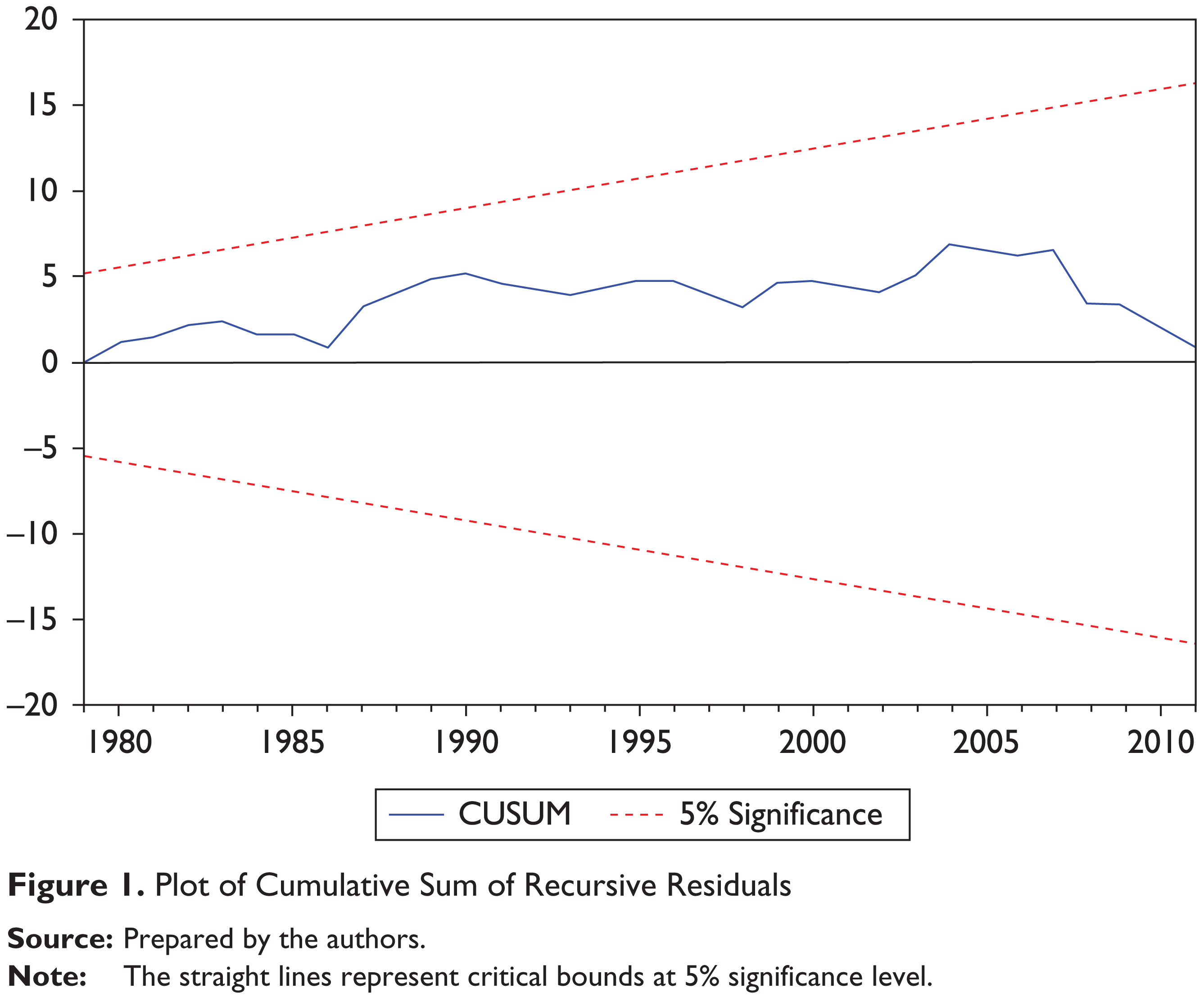
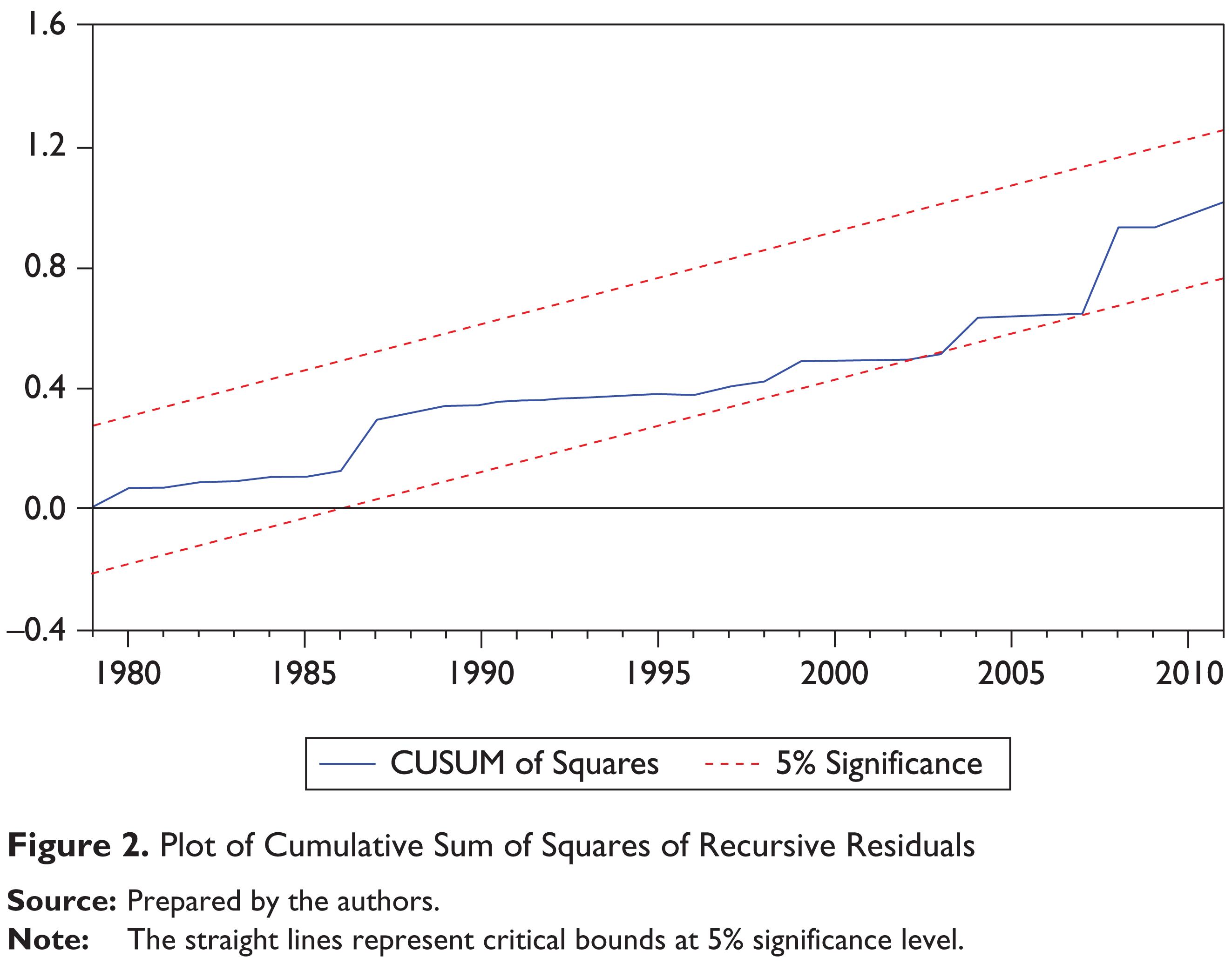
The CUSUM and CUSUMsq tests are used to examine the stability of the long- and short-term parameters. If the plots of the graph for both the tests lie within 5 per cent critical bounds, we accept the hypothesis that ‘the regression equation is correctly specified’ (Bahmani-Oskooee & Nasir, 2004, p. 485). Our results are within the critical bounds (Figures 1 and 2). Thus the model is stable and correctly specified.

Figure 1.

Source: Prepared by the authors.

Figure 2.

Source: Prepared by the authors.

Generalized Variance Decomposition

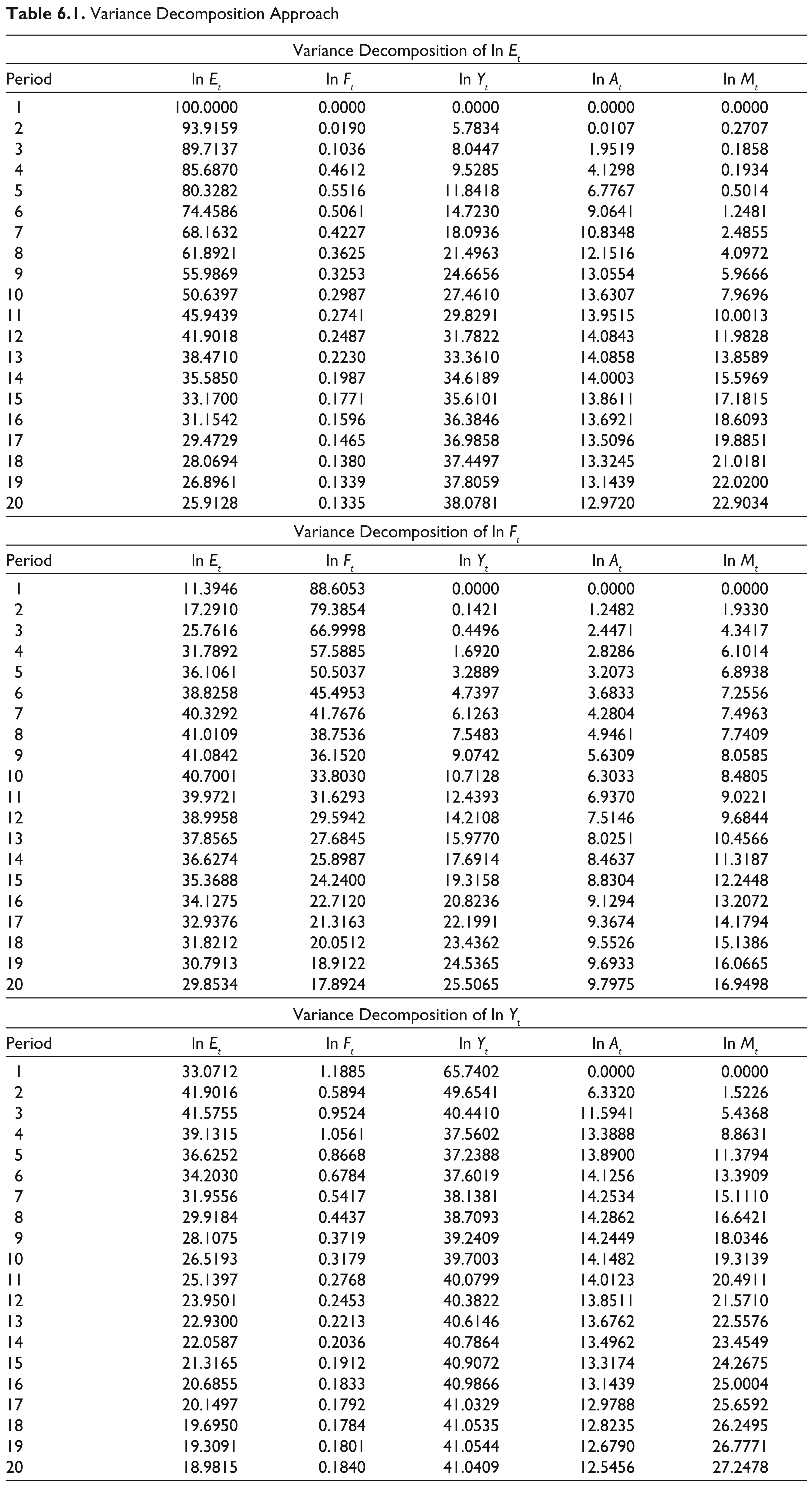
By implementing the IAA, we find that 25.91 per cent energy consumption is explained by its own innovative shocks, 0.13 per cent by financial development and 38.07 per cent by economic growth. Financial development explains very small part of energy consumption through the innovative shocks. The contribution of agriculture growth and growth in modern sector to energy consumption is 12.97 per cent and 22.90 per cent, respectively.

This implies that next to economic growth and growth in modern sector are the major drivers of energy consumption. The share of energy consumption to explain financial development is 29.85 per cent, but 17.89 per cent portion of financial development is contributed by its own innovative shocks. One innovative shock in economic growth explains financial development by 25.50 per cent. Agriculture growth and growth in modern sector contribute to financial development by 9.79 and 16.94 per cent, respectively, through their innovative shocks.

We found that energy consumption causes financial development in the Granger sense. This is consistent with Dan and Lijun (2009) who found the unidirectional causality from energy consumption to financial development, but Shahbaz and Lean (2012a) and Islam et al. (2013) reported the feedback effect between the two series for Tunisia and Malaysia, respectively. One standard deviation shock to energy consumption explains 18.98 per cent of economic growth, but a shock to financial development on economic growth is negligible. Growth in agriculture and modern sectors significantly adds to economic growth, that is, 27.24 and 12.54 per cent, respectively.

We find bidirectional causality between energy consumption and economic growth but strong causality running from economic growth to energy consumption. This finding is consistent with Alam and Butt (2002), Shahbaz and Lean (2012b) and Shahbaz, Zeshan and Afza (2012). The finding that economic growth causes financial development lends support to the demand-side hypothesis, something that was reported by Shahbaz (2012) for Pakistan.

A look at Table 6 shows the impact of shock. Energy consumption explains 30 per cent of agriculture growth from its own innovative shocks, while financial development explains 5.41 per cent of agriculture growth. Innovative shocks to economic growth explain 26.92 per cent of agriculture growth. Growth in modern sector adds to agriculture growth by 12.33 per cent, and 25.76 per cent is explained by innovative shocks to agriculture growth itself. We find unidirectional causality from energy consumption to agriculture growth. This finding is consistent with Mushtaq et al. (2007). They reported that electricity consumption in agricultural sector plays a critical in boosting the productivity of agriculture sector. Sebri and Abid (2012) found that energy consumption Granger causes agricultural growth in Tunisia. Faridi (2012) reported unidirectional causality from agriculture growth to economic growth. The author argued that agricultural productivity helps to promote rural economic activity and contributes to economic growth.

Table 6 shows that a sizeable part of the growth in modern sector is explained by the innovative shocks of energy consumption, but financial development contributes minimally to it. A 37.90 per cent growth in modern sector is explained by innovative shocks to economic growth, while 11.09 and 28.25 per cent are explained by the innovative shocks in agriculture growth and growth in modern sector, respectively. The contribution of financial development and agriculture growth is dismal. We find bidirectional link between energy consumption and growth in modern sector and same is true for economic growth and growth in modern sector.

Table 6.1.

Variance Decomposition Approach

Variance Decomposition of ln E_t
Period	ln E_t	ln F_t	ln Y_t	ln A_t	ln M_t
1	100.0000	0.0000	0.0000	0.0000	0.0000
2	93.9159	0.0190	5.7834	0.0107	0.2707
3	89.7137	0.1036	8.0447	1.9519	0.1858
4	85.6870	0.4612	9.5285	4.1298	0.1934
5	80.3282	0.5516	11.8418	6.7767	0.5014
6	74.4586	0.5061	14.7230	9.0641	1.2481
7	68.1632	0.4227	18.0936	10.8348	2.4855
8	61.8921	0.3625	21.4963	12.1516	4.0972
9	55.9869	0.3253	24.6656	13.0554	5.9666
10	50.6397	0.2987	27.4610	13.6307	7.9696
11	45.9439	0.2741	29.8291	13.9515	10.0013
12	41.9018	0.2487	31.7822	14.0843	11.9828
13	38.4710	0.2230	33.3610	14.0858	13.8589
14	35.5850	0.1987	34.6189	14.0003	15.5969
15	33.1700	0.1771	35.6101	13.8611	17.1815
16	31.1542	0.1596	36.3846	13.6921	18.6093
17	29.4729	0.1465	36.9858	13.5096	19.8851
18	28.0694	0.1380	37.4497	13.3245	21.0181
19	26.8961	0.1339	37.8059	13.1439	22.0200
20	25.9128	0.1335	38.0781	12.9720	22.9034
Variance Decomposition of ln F_t
Period	ln E_t	ln F_t	ln Y_t	ln A_t	ln M_t
1	11.3946	88.6053	0.0000	0.0000	0.0000
2	17.2910	79.3854	0.1421	1.2482	1.9330
3	25.7616	66.9998	0.4496	2.4471	4.3417
4	31.7892	57.5885	1.6920	2.8286	6.1014
5	36.1061	50.5037	3.2889	3.2073	6.8938
6	38.8258	45.4953	4.7397	3.6833	7.2556
7	40.3292	41.7676	6.1263	4.2804	7.4963
8	41.0109	38.7536	7.5483	4.9461	7.7409
9	41.0842	36.1520	9.0742	5.6309	8.0585
10	40.7001	33.8030	10.7128	6.3033	8.4805
11	39.9721	31.6293	12.4393	6.9370	9.0221
12	38.9958	29.5942	14.2108	7.5146	9.6844
13	37.8565	27.6845	15.9770	8.0251	10.4566
14	36.6274	25.8987	17.6914	8.4637	11.3187
15	35.3688	24.2400	19.3158	8.8304	12.2448
16	34.1275	22.7120	20.8236	9.1294	13.2072
17	32.9376	21.3163	22.1991	9.3674	14.1794
18	31.8212	20.0512	23.4362	9.5526	15.1386
19	30.7913	18.9122	24.5365	9.6933	16.0665
20	29.8534	17.8924	25.5065	9.7975	16.9498
Variance Decomposition of ln Y_t
Period	ln E_t	ln F_t	ln Y_t	ln A_t	ln M_t
1	33.0712	1.1885	65.7402	0.0000	0.0000
2	41.9016	0.5894	49.6541	6.3320	1.5226
3	41.5755	0.9524	40.4410	11.5941	5.4368
4	39.1315	1.0561	37.5602	13.3888	8.8631
5	36.6252	0.8668	37.2388	13.8900	11.3794
6	34.2030	0.6784	37.6019	14.1256	13.3909
7	31.9556	0.5417	38.1381	14.2534	15.1110
8	29.9184	0.4437	38.7093	14.2862	16.6421
9	28.1075	0.3719	39.2409	14.2449	18.0346
10	26.5193	0.3179	39.7003	14.1482	19.3139
11	25.1397	0.2768	40.0799	14.0123	20.4911
12	23.9501	0.2453	40.3822	13.8511	21.5710
13	22.9300	0.2213	40.6146	13.6762	22.5576
14	22.0587	0.2036	40.7864	13.4962	23.4549
15	21.3165	0.1912	40.9072	13.3174	24.2675
16	20.6855	0.1833	40.9866	13.1439	25.0004
17	20.1497	0.1792	41.0329	12.9788	25.6592
18	19.6950	0.1784	41.0535	12.8235	26.2495
19	19.3091	0.1801	41.0544	12.6790	26.7771
20	18.9815	0.1840	41.0409	12.5456	27.2478

Table 6.2.

Variance Decomposition Approach

Variance Decomposition of ln A_t
Period	ln E_t	ln F_t	ln Y_t	ln A_t	ln M_t
1	6.6057	0.1129	13.1645	80.1166	0.0000
2	9.2050	4.2687	14.1642	72.3535	0.0084
3	19.6619	7.3192	12.4901	60.4870	0.0422
4	24.6398	11.3347	10.9318	52.9898	0.1037
5	30.2862	12.7219	9.76694	47.0948	0.1300
6	34.4551	12.9375	9.1805	43.2462	0.1806
7	37.3312	12.5638	9.1184	40.7314	0.2551
8	39.2398	11.9964	9.4606	38.9347	0.3683
9	40.2761	11.3678	10.2033	37.5866	0.5659
10	40.6202	10.7280	11.2931	36.4641	0.8945
11	40.3938	10.0949	12.6853	35.4224	1.4033
12	39.7123	9.4715	14.3146	34.3786	2.1226
13	38.6920	8.8605	16.0941	33.2970	3.0561
14	37.4429	8.2665	17.9337	32.1754	4.1813
15	36.0660	7.6964	19.7509	31.0307	5.4557
16	34.6462	7.1577	21.4810	29.8880	6.8270
17	33.2484	6.6567	23.0799	28.7723	8.2424
18	31.9183	6.1980	24.5233	27.7048	9.6554
19	30.6839	5.7835	25.8030	26.7005	11.0289
20	29.5597	5.4133	26.9220	25.7685	12.3363
Variance Decomposition of ln A_t
Period	ln E_t	ln F_t	ln Y_t	ln A_t	ln M_t
1	13.5970	3.3669	33.5980	4.3612	45.0768
2	28.3096	3.6989	31.2900	5.6410	31.0603
3	31.7590	3.5608	31.0216	6.0269	27.6315
4	32.8176	3.2727	30.8897	7.0302	25.9895
5	32.9959	3.0417	30.9471	7.9108	25.1043
6	32.5513	2.7657	31.3870	8.6334	24.6624
7	31.8244	2.4812	31.9970	9.2339	24.4633
8	30.9253	2.2183	32.6899	9.7211	24.4451
9	29.9414	1.9873	33.4025	10.1146	24.5540
10	28.9343	1.7898	34.0929	10.4256	24.7572
11	27.9434	1.6224	34.7380	10.6653	25.0307
12	26.9959	1.4809	35.3239	10.8445	25.3546
13	26.1083	1.3613	35.8451	10.9729	25.7122
14	25.2898	1.2599	36.3009	11.0597	26.0894
15	24.5443	1.1740	36.6941	11.1130	26.4744
16	23.8718	1.1013	37.0290	11.1401	26.8576
17	23.2696	1.0398	37.3116	11.1472	27.2316
18	22.7335	0.9879	37.5477	11.1395	27.5911
19	22.2586	0.9444	37.7437	11.1210	27.9321
20	21.8392	0.9080	37.9052	11.0951	28.2523

Source: Prepared by the author.

Generalized Impulse Response Function

The generalized IRF shows responsiveness of the regressands to shocks to each series within the VAR model. The plots in IRF (Figure 3) indicate that the response of energy consumption to a unit standard deviation shock in financial development is weak, but strong in the reverse direction—case of unidirectional causality. The response of energy consumption from shocks in economic growth and growth in modern sector is very strong and positive. Energy consumption and growth in modern sector contribute to economic growth positively and strongly. This confirmed our established bidirectional causality between energy consumption and economic growth and energy consumption and growth in modern sector. Feedback effect exists between economic growth and modern sector growth. The response of energy consumption from one standard shock to agriculture growth is depleting, while financial development responds positively and strongly to standard shocks in energy consumption. This establishes a causal link between energy consumption and financial development. The response of energy consumption, financial development and economic growth due to standard shocks stemming from agriculture growth is undetermined.

Figure 3.

Source: Prepared by the authors.

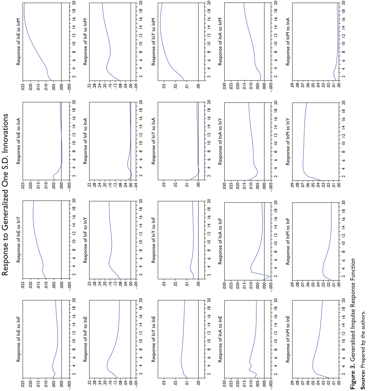
Agriculture growth responds positively from a unit standard error random shock to financial development, but it is significant. Energy consumption, economic growth and growth in modern sector add to agriculture growth positively. Finally, modern sector growth strongly responds to unit standard error random shocks in energy consumption, financial development and economic growth but is weak due to shocks occurring in agriculture growth. The results of IRF are very similar to those found from variance decomposition methods.

Conclusion and Policy Implications

The article finds a long-run equilibrium relationship among energy consumption, financial development, economic growth, growth in agriculture and modern sectors in Pakistan from 1972 to 2011. Ng–Perron test shows that all the series are I(1). The ZA test identifies structural break in the series. The ARDL bounds testing approach has been used to find the long-run relation and the IAA for the direction of causality. Evidence points to a significant positive impact of financial development on energy consumption, and economic growth further adds to it. Agriculture growth increases demand for energy but growth in modern sector does the opposite. The IAA shows unidirectional causality from energy consumption to financial development and bidirectional causality between economic growth and energy consumption. Financial development is Granger caused by economic growth. Energy consumption and economic growth Granger cause agriculture growth. The feedback effect exists between energy consumption and growth in modern sector and the same is true for growth in modern sector and economic growth.

Contemporary research suggests that financial development is a major driver of economic growth in emerging nations and has a significant impact on energy consumption. The literature on financial development and economic growth points to the role of finance in economic activity. The energy literature points to the link between energy and economic growth. In a free market economy, entrepreneurial talents are translated to action through access to finance. A financially developed system facilitates resources’ availability for viable investment projects. The latter stimulates economic growth which in turn raises demand for energy. While intuitively appealing, the article finds empirical support to this idea.

The findings of the study can help to formulate appropriate policy and promote economic growth in Pakistan. A developed financial system attracts investors, boosts stock market and channels funds to the sectors that are more efficient. Modernizing capital equipment will lower energy use and help to achieve productive efficiency. The long-run coefficients are larger than (still small) those for the short run which appears to be more of a structural issue and should be addressed based on further research.

In Pakistan, poorly designed ad hoc macroeconomic policies relating to stock markets and deteriorating law and order situation have been a recipe for a corrosive chemistry. These factors contribute to the poor economic performance. The stock market is in need of overhaul to create a pro-business atmosphere that will help in confidence building at home and abroad. Without suggesting too much regulation in the financial sector of Pakistan, one can still introduce sensible albeit comprehensive financial reforms to strengthen the sector and achieve efficiency. The government should introduce broad incentives to local and foreign investors. The commercial banking sector should extend more support to importers of modern technology for the industrial sector. Energy-efficient technology should be given serious consideration which can save energy and lower energy intensity.

Resources should be allocated to research and development for exploring new sources of energy for sustainable economic development. Modern sector should focus on green energy to address environmental concerns. Modernization of technology will boost agricultural growth and should be encouraged and supported. Training at rural areas to train farmers in this regard would be helpful. More agricultural development should be considered.

For the future, research should explore the relationship between economic growth, financial development and energy consumption from the perspective of sectors. In this case, it would be necessary to use sectoral data which may help policymakers to design comprehensive economic, financial and energy policy for sustained growth by sector. This would allow a macro-approach from a micro-level. The relationship among these series should also be examined using panel methodology for more reliable estimates. Shahbaz (2012) points out that for optimal fruits of financial liberalization or financial development, sensible and yet careful trade openness must be on the menu. However, a word of admonition from Bhagwati (2002, p. 180) is in order here.

While freer trade, or ‘openness’ in trade, is now widely regarded as economically benign, in the sense that it increases the size of the pie, the recent anti-globalization critics have suggested that it is socially malign on several dimensions, among them the question of poverty. Their contention is that trade accentuates not ameliorates, deepens not diminishes, poverty in both the rich and the poor countries. The theoretical and empirical analysis of the impact of freer trade on poverty in the rich and in the poor countries is not symmetric, of course.

Footnotes

Acknowledgements

The authors are grateful to the anonymous referees of the journal for their extremely useful suggestions to improve the quality of the article. Usual disclaimers apply.

Notes

References

Abu-Bader

, & Abu-Qarn

A.S.

(2008). Financial development and economic growth: The Egyptian experience. Journal of Policy Modeling, 30(5), 887–898.

Alam

, & Butt

M.S.

(2002). Causality between energy consumption and economic growth in Pakistan: An application of co-integration and error correction modeling techniques. Pacific and Asian Journal of Energy, 12(3), 151–165.

Apergis

, & Payne

J.E.

(2009a). Energy consumption and economic growth in Central America: Evidence from a panel cointegration and error correction model. Energy Economics, 31(2), 211–216.

Apergis

, & Payne

J.E.

(2009b). Energy consumption and economic growth: Evidence from the Commonwealth of Independent States. Energy Economics, 31(5), 641–647.

Apergis

, & Payne

J.E.

(2010). Energy consumption and growth in South America: Evidence from a panel error correction model. Energy Economics, 32(6), 1421–1426. doi:10.1016/j.eneco.2010.04.006.

Aqeel

, & Butt

M.S.

(2001). The relationship between energy consumption and economic growth in Pakistan. Asia-Pacific Development Journal, 8(2), 101–10.

Bahmani-Oskooee

, & Nasir

A.M.

(2004). ARDL approach to test the productivity bias hypothesis. Review of Development Economics, 8(3), 483–488.

Bairer

S.L

, Dwyer

G.P.

Jr. , & Tamura

(2004). Does opening a stock exchange increase economic growth? Journal of International Money and Finance, 23(3), 311–331.

Bannerjee

, Dolado

, & Mestre

(1998). Error-correction mechanism tests for cointegration in single equation framework. Journal of Time Series Analysis, 19(3), 267–283.

10.

Bartleet

, & Gounder

(2010). Energy consumption and economic growth in New Zealand: Results of trivariate and multivariate models. Energy Policy, 38(7), 3505–3517.

11.

Beakert

& Harvey

C.R.

(2000). Foreign speculators and emerging equity markets. Journal of Finance, 52(2), 565–614.

12.

Beakert

, Harvey

C.R.

& Lumsdaine

R.L.

(2002). Dating the integration of world equity markets. Journal of Financial Economics, 65(2), 203–247.

13.

Beakert

, Harvey

C. R.

& Lundblad

(2001). Emerging equity markets and economic development. Journal of Development Economics, 66(2), 465–504.

14.

Beakert

, Harvey

C. R.

& Lundblad

(2005). Does financial liberalization spur growth? Journal of Financial Economics, 77(1), 3–55.

15.

Beaudreau

B.C.

(2005). Engineering and economic growth. Structural Change and Economic Dynamics, 16(2), 211–220.

16.

Beaudreau

B.C.

(2010). On the methodology of energy-GDP Granger causality tests. Energy, 35(9), 3535–3539.

17.

Bencivenga

V.R.

, & Smith

B.D.

(1991). Financial intermediation and endogenous growth. The Review of Economic Studies, 58(2), 195–209.

18.

Bhagwati

(2002). Free Trade Today. Princeton, NJ: Princeton University Press.

19.

Bhargava

(1986). On the theory of testing for unit roots in observed time series. The Review of Economic Studies, 53(3), 369–384.

20.

Bowden

& Payne

J.E.

(2009). The causal relationship between U.S. energy consumption and real output: A disaggregated analysis. Journal of Policy Modeling, 31(2), 180–188.

21.

Chtioui

(2012). Does economic growth and financial development spur energy consumption in Tunisia? Journal of Economics and International Finance, 4(4), 150–158.

22.

Coban

, & Topcu

(2013). The nexus between financial development and energy consumption in the EU: A dynamic panel data analysis. Energy Economics, 39(2), 81–88.

23.

Dan

, & Lijun

(2009). Financial development and energy consumption: An empirical research based on Guangdong Province. Paper presented at International Conference on Information Management, Innovation Management and Industrial Engineering, 2009, ICIII, 3, pp. 102–105.

24.

Elliot

, Rothenberg

T.J.

, & Stock

J.H.

(1996). Efficient tests for an autoregressive unit root. Econometrica, 64(4), 813–836.

25.

Enders

(1995). Applied econometric time series. New York, NY: Wiley.

26.

Faridi

M.Z.

(2012). Contribution of Agricultural Exports to Economic Growth in Pakistan. Pakistan Journal of Commerce and Social Science, 6(1), 133–146.

27.

Fatai

, Oxley

, & Scrimgeour

F.G.

(2004). Modelling the causal relationship between energy consumption and GDP in New Zealand, Australia, India, Indonesia, The Philippines and Thailand. Mathematics and Computers in Simulation, 64(3–4), 431–445.

28.

Fung

H.K.

(2009). Financial development and economic growth: convergence or divergence? Journal of International Money and Finance, 28(1), 56–78.

29.

Greenwood

, & Jovanovich

(1990). Financial development, growth, and the distribution of income. Journal of Political Economy, 98(5), 1076–1107.

30.

Halicioglu

(2009). An Econometric Study of CO2 Emissions, Energy Consumption, Income and Foreign Trade in Turkey. Energy Policy, 37(3), 1156–1164.

31.

Ibrahim

M.H.

(2007). The role of the financial sector in economic development: The Malaysian case. International Review of Economics, 54(4), 463–483.

32.

Islam

, Shahbaz

, Ahmed

, & Alam

(2013). Financial development and energy consumption nexus in Malaysia: A multivariate time series analysis. Economic Modelling, 30(1), 435–441.

33.

Karanfil

(2009). How many times again will we examine the energy–income nexus using a limited range of traditional econometric tools? Energy Policy, 36(4), 3019–3025.

34.

Khan

A.M.

, & Qayyum

(2007). Dynamic modeling of energy and growth in South Asia. The Pakistan Development Review, 46(4), 481–498.

35.

King

R.G.

& Levine

(1993). Finance and growth: Schumpeter might be right. Quarterly Journal of Economics, 108(3), 717–738.

36.

Kraft

, & Kraft

(1978). On the relationship between energy and GNP. Journal of Energy and Development, 3(2), 401–403.

37.

Lee

C.C.

, & Chang

C.P.

(2008). Energy consumption and economic growth in Asian economies: A more comprehensive analysis using panel data. Resources and Energy Economics, 30(1), 50–65.

38.

Levine

(1997). Financial development and economic growth: views and agenda. Journal of Economic Literature, 35(2), 688–726.

39.

Mankiw

N.G.

& Scarth

(2008). Macroeconomics: Third Canadian EditionWorth Publishers. New York.

40.

McKinnon

R.I.

(1973). Money and capital in economic development. Washington, DC: Brookings Institution.

41.

Mehrara

, & Musai

(2012). Energy consumption, financial development and economic growth: An ARDL approach for the case Iran. International Journal of Business and Behavioral Sciences, 2(2), 92–99.

42.

Minier

(2009). Opening a stock exchange. Journal of Development Economics, 90(24), 135–143.

43.

Mishra

, Smyth

, & Sharma

(2009). The energy-GDP nexus: Evidence from a panel of Pacific Island countries. Resource and Energy Economics, 31(3), 210–220.

44.

Mushtaq

, Abbas

, & Abedullah

Ghafoor A.

(2007). Energy use for economic growth: Cointegration and causality analysis from the agriculture sector in Pakistan. The Pakistan Development Review, 46(4), 1065–1075.

45.

Narayan

P.K.

(2005). The saving and investment nexus for China: Evidence from cointegration tests. Applied Economics, 37(17), 1979–1990.

46.

Narayan

P.K.

& Narayan

(2004). Is there a long-run relationship between exports and imports? Evidence from two pacific island countries. Economic Papers, 23(2), 152–164.

47.

, & Perron

(2001). Lag length selection and the construction of unit root test with good size and power. Econometrica, 69(6), 1519–1554.

48.

Odhiambo

N.M.

(2010). Finance-investment-growth nexus in South Africa: An ARDL-bounds testing procedure. Economic Change and Restructuring, 43(3), 205–219.

49.

, & Lee

(2004). Causal relationship between energy consumption and GDP revisited: The case of Korea 1979–1999. Energy Economics, 26(4), 51–59.

50.

Ouattara

(2004). Foreign aid, public savings displacement, and aid dependency in Côte d’Ivoire: an aid disaggregation approach (Discussion Paper Series 0406). The School of Economics, The University of Manchester.

51.

Patrick

H.T.

(1966). Financial development and economic growth in underdeveloped countries. Economic Development and Cultural Change, 14(2), 174–187.

52.

Perron

& Vogelsang

T.J.

(1992). Nonstationarity and level shifts with an application to purchasing power parity. Journal of Business and Economic Statistics, 10(3), 301–320.

53.

Pesaran

M.H.

, Shin

, & Smith

(2001). Bounds testing approaches to the analysis of level relationships. Journal of Applied Econometrics, 16(3), 289–326.

54.

Phillips

P.C.B.

, & Perron

(1988). Testing for a unit root in time series regression. Econometrica, 75(2), 355–346.

55.

Qazi

M.A.H.

, & Riaz

(2008). Causality between energy consumption and economic growth: the case of Pakistan. Lahore Journal of Economics, 13(2), 45–58.

56.

Sadorsky

(2010). The impact of financial development on energy consumption in emerging economies. Energy Policy, 38(5), 2528–2535.

57.

Sadorsky

(2011). Financial Development and Energy Consumption in Central and Eastern European Frontier Economies. Energy Policy, 39(2), 999–1006.

58.

Shahbaz

(2009). A reassessment of finance-growth nexus for Pakistan: under the investigation of FMOLS and DOLS techniques. The IUP Journal of Applied Economics, 0(1), 65–80.

59.

Shahbaz

(2012). Does trade openness affect long run growth? Cointegration, causality and forecast error variance decomposition tests for Pakistan. Economic Modelling, 29(6), 2325–2339.

60.

Shahbaz

, & Lean

H.H.

(2012a). Does financial development increase energy consumption? The role of industrialization and urbanization in Tunisia. Energy Policy, 40(1), 473–479.

61.

Shahbaz

, & Lean

H.H.

(2012b). The dynamics of electricity consumption and economic growth: A revisit study of their causality in Pakistan. Energy, 39(1), 146–153.

62.

Shahbaz

& Malik

M.N.

(2011). Does financial instability weaken the finance-growth nexus? a case for Pakistan. 2nd International Conference on Business and Economic Research (2nd ICBER 2011) Proceeding 2011–174, Conference Master Resources.

63.

Shahbaz

, & Rahman

M.M.

(2012). The dynamic of financial development, imports, foreign direct investment and economic growth: Cointegration and causality analysis in Pakistan. Global Business Review, 13(2), 201–219.

64.

Shahbaz

, Saleheen

, & Tahir

M.I.

(2013). The dynamic link between energy consumption, economic growth, financial development and trade in China: fresh evidence from multivariate framework analysis. Energy Economics, 40(2), 8–21.

65.

Shahbaz

, Shamim

S.M.A.

& Aamir

(2010a). Macroeconomic environment and financial sector’s performance: Econometric evidence from three traditional approaches. The IUP Journal of Financial Economics, (1&l2), 103–123.

66.

Shahbaz

, Zeshan

, & Afza

(2012a). Is energy consumption effective to spur economic growth in Pakistan? New evidence from bounds test to level relationships and Granger causality tests. Economic Modelling, 29(6), 2310–2319.

67.

Shan

(2005). Does financial development ‘lead’ economic growth? A vector auto-regression appraisal. Applied Economics, 37(12), 1353–1367.

68.

Shrestha

, & Chowdhury

(2005). ARDL modeling approach to testing the financial liberalization hypothesis (University of Wollongong Economics Working Paper Series 2005). Faculty of Business, University of Wollongong.

69.

Siddiqui

(2004). Energy and economic growth in Pakistan. The Pakistan Development Review, 43(4), 175–200.

70.

Stern

D.I.

(1993). Energy and economic growth in U.S.A. Energy Economics, 15(2), 137–150.

71.

Stern

D.I.

(2000). Multivariate cointegration analysis of the role of energy in the U.S macroeconomy. Energy Economics, 22(2), 267–283.

72.

Stern

D.I.

(2004). The rise and fall of the environmental Kuznets curve. World Development, 32(8), 1419–1439.

73.

Tang

S.F.

& Tan

B.W.

(2014). The linkages among energy consumption, economic growth, relative price, foreign direct investment, and financial development in Malaysia. Quality and Quantity, 48(2), 781–797.

74.

Townsend

R.M.

(1979). Optimal contracts and competitive markets with costly state verification. Journal of Economic Theory, 21(4), 265–293.

75.

Wachtel

, Hasan

, & Zhou

(2006). Institutional development, financial deepening and economic growth: Evidence from China (BOFIT Discussion Paper No. 12/2006). Finland: Institute for Economies in Transition, Bank of Finland.

76.

Wolde–Rufael

(2009). Energy consumption and economic growth: the experience of African countries revisited. Energy Economics 31(2), 217–224.

77.

World Development Indicators (WDI-CD, 2012). Retrieved from http://data.worldbank.org/products/wdi

78.

(2012). The impact of financial development on energy consumption in China: Based on SYS-GMM estimation. Advanced Materials Research, 524–527, 2977–2981.

79.

Yang

H.Y.

(2000). A note of the causal relationship between energy and GDP in Taiwan. Energy Economics, 22, 309–317.

80.

Yildirim

, Aslan

, & Ozturk

(2012). Coal consumption and industrial production nexus in USA: Cointegration with two unknown structural breaks and causality approaches. Renewable and Sustainable Energy Reviews, 16(8), 6123–6127.

81.

Yoo

(2006). The causal relationship between electricity consumption and economic growth in ASEAN countries. Energy Policy, 34(18), 3573–3582.

82.

S.H.

, & Choi

J.Y.

(1985). The causal relationship between energy and GNP: An international comparison. Journal of Energy and Development, 11(2), 249–272.

83.

Zicchino

(2006). A model of bank capital, lending and the macroeconomy: Basel I versus basel Ii. Manchester School, 74(1), 50–77.

84.

Zivot

, & Andrews

(1992). Further evidence on the great crash, the oil price shock, and the unit root hypothesis. Journal of Business Economics and Statistics, 10 (3), 251–270.