More Finance or Better Finance in Feldstein–Horioka Puzzle: Evidence from SSA Countries

Abstract

This study examined the role of financial development in the Feldstein–Horioka (FH) puzzle for 31 sub-Saharan African (SSA) countries for the period 1999–2011. Unlike previous studies that used traditional measures of finance (‘more finance’), we advocated for superior measures of financial development (‘better finance’). The baseline regression shows that ‘more finance’ increases the FH estimate, while ‘better finance’ serves as drag to the same retention coefficients. The reverse of these results was obtained when the baseline regression was extended to account for the interaction between savings and proxies for finance. The results obtained show a considerable improvement in the saving retention coefficient when ‘better finance’ was used as against ‘more finance’. This concretely reinforces the superior role of ‘better finance’ in mobilizing, distributing and utilizing savings for investment within these economies. Based on these findings, domestic resource mobilization can be a veritable vehicle for plugging the substantial investment gap in these SSA economies. However, such policy thrust must be complemented by far-reaching financial reforms.

Keywords

Feldstein–Horioka coefficient panel regression financial development fixed effect sub-Saharan Africa

Introduction

In 1980, Feldstein and Horioka (FH) measured capital mobility by examining the correlation between domestic savings and investment for 16 Organisation for Economic Co-operation and Development (OECD) countries. They argued that in a world of unfettered capital mobility, domestic savings would flow to countries with the highest rate of return and domestic savings would be financed by world pool of savings. This serves as the basis for making the assumption that in a situation of capital immobility (mobility), the correlation between investment and savings, otherwise referred to as ‘retention coefficient’, must tend to unity (zero). In other words, a country that is in financial autarky would source for investment fund from domestic savings. The ensuing contradiction between empirical and theoretical wisdom coined the conventional FH puzzle, which Obstfeld and Rogoff (2000) tagged as the ‘mother of all puzzles’.¹

A survey of the literature on the FH puzzle elicits that there are two major strands. In the first strand are a group of studies that validate FH puzzle and conclude that measuring capital mobility as prescribed by FH based on policy regime would introduce bias into the model (Bajo-Rubio, 1998; Coakley, Fuertes & Spagnolo, 2004; Gundlach & Sinn, 1992; Jansen, 1996; Jansen & Schulze, 1996; Mastroyiannis, 2007; Ozmen & Parmaksiz, 2003; Sarno & Taylor, 1998). The second strand relates to studies that refute FH puzzle on factors that are unrelated to capital mobility and thus argue that FH approach of measuring capital mobility is wrong. For instance, the influential study by Coakley, Kulasi and Smith (1998) accounts for current account solvency constraints. Obstfeld (1985) focused on the growth rate of income. Using threshold variable, Ho (2003) limited his study to country size, while Fouquau, Hurlin and Rabaud (2008) considered the threshold level for economic growth, demography, degree of openness, country size and current account balance. Adeniyi and Egwaikhide (2013) introduced financial development, while Özmen (2004) expanded the model to capture exchange rate regime. Raheem, Adeniyi and Ajide(2016) factor in the role of governance in the FH puzzle.

This present study takes a cue from the second strand of literature. Specifically, this study seeks to inquire the role of financial development in the savings–investment nexus. The importance of a sound financial system cannot be overemphasized in economic growth issues. McKinnon (1973) and Shaw (1973) posit that the key function of a financial intermediary is to channel capital from the surplus unit of the economy to the deficit unit of the economy. Similarly, Demirgüç-Kunt (2008), as cited by Raheem and Oyinlola (2015), opines that the overall function of a financial system is to reduce information and transaction costs impeding economic activity, and its five core functions are to produce ex ante information about possible investments and allocate capital; monitor investments and provide corporate governance after providing finance; facilitate trading, diversification and management of risk; mobilize and pool savings; and ease the exchange of goods and services.

The positive effects of financial development indicators on aggregate productivity have been established in the literature.² This view is consistent with the proposition of ‘more finance, more growth’. These indicators can be faulted on two grounds. First, the recent global financial crisis showcased the possibilities of malfunctioning financial system to directly or indirectly waste resources, discourage savings and encourage speculation, hence resulting in decline in investment and misallocation of scarce resources (Law & Singh, 2014; Law, Azman-Saini & Ibrahim, 2013). This being the case, one of the functions of the financial system and the financial intermediary would be altered.

Second, the conventional financial development indicators measure the size of the financial system and have nothing to say as regards efficiency of the system. Arestis and Demetriades (1996) and Demetriades and Andrianova (2004) in their papers underscored that varying connections may reflect dissimilarities in the quality of finance, which is determined by the quality of financial regulation and rule of law. Cooray (2012) was of the view that efficiency of the financial sector is a better measure than the size of the sector. Bettin and Zazzaro (2009) and Raheem (2015) opined that the qualitative measure of financial development (efficiency) would be able to capture satisfactorily the microeconomic efficiency of banks, a fundamental characteristic that the quantitative approach lacks. For example, the traditional indicators lack the ability to select entrepreneur and channel savings towards high-profit investment ventures. Hence, this will help ameliorate the negative net present value projects by banks that are accompanied by lower cost (credit) from the banks. The relationship between efficiency of a financial sector and economic growth can be coined ‘better finance, more growth’. Based on the foregoing, it can be hypothesized that ‘better finance, more growth’ is a superior measure of the financial system, when compared to ‘more finance-more growth’.

The objective of the study is to extend the work of Adeniyi and Egwaikhide (2013) by providing different and possibly better proxies for financial development. As such, it seeks to determine which of the indicators (‘more finance’ or ‘better finance’) matters most in the ‘mother of all puzzles’. This crux of the study serves as the value addition to the literature, as no study we are aware of has considered the importance of ‘better finance’ indicators in the saving–investment nexus.

Following the introductory section, the rest of the article is structured into the following sections. The second section dwells on the methodology and data-related issues. We present the empirical results of the estimated models in the third section, while the fourth section highlights the concluding remarks as well as policy implications of the study.

Data and Methodology

The second section of this study is trifurcated into three subsections. The first highlights a brief description of the financial sector indicators often used by previous studies. The second subsection dwells on the new indicators as argued above (i.e., financial efficiency indicators or ‘better finance’). The last part of the section focuses on model specification as well as estimation procedures.

Data-related Issues on Financial Development

The financial system is comprised of both money and capital markets. As such, it is expected that both markets would have their individual indicators to quantify their development. The money market can be further broken down into three major sectors/industries, which are banking, insurance and bureau de change. Of these three industries, the banking sector is the most sophisticated and regulated sector. The most common indicators used are domestic credit to the private sector, liquidity liabilities (M3) and domestic credit provided by the banking sector. Based on the definition of the World Bank, M3 is the sum of currency and deposits in the central bank (M0), transferable deposits and electronic currency (M1), time and savings deposits, foreign currency transferable deposits, certificates of deposit, securities repurchase agreements (M2), travellers cheques, foreign currency time deposits, commercial paper and shares of mutual funds or market funds held by residents. It thus provides an encompassing measure of the overall size of the financial sector. Domestic credit to private sector refers to financial resources provided to the private sector, such as through loans, purchases of non-equity securities and trade credits and other accounts receivable that establish a claim for repayment. For some countries, these claims include credit to public enterprises. The last indicator, domestic credit provided by the banking sector includes all credit to various sectors on a gross basis, with the exception of credit to the central government.

The capital market essentially deals with bonds and stocks of both the government and private users. The most common indicators used are stock market capitalization, which is defined as the product of share price and the number of shares outstanding in companies listed on the country’s domestic stock exchange at the end of the year. The second indicator is stock traded value, which refers to the total value of shares traded during the period. There is also stock market turnover ratio, which is defined as the deflated ratio of the value of total shares traded to average real market capitalization.

A survey of literature has shown that existing studies are biased towards the use of money market-based indicators of which domestic credit to the private sector has been used in all existing studies For instance, Shahbaz and Rahman (2012) used the conventional measures of financial development, while Tripathy and Pradhan (2014) limited their measure to banking sector only. However, Yartey and Adjasi (2007) based their study solely on capital market indicators for 19 exchanges in SSA.

Financial Efficiency Indicator and Measurement

Based on the deficiency and unsatisfactory performance of ‘more finance’ indicators, individuals as well as organizations have taken it upon themselves to find better measures that would capture satisfactorily the development of the financial system. Beck, Demirguc-Kunt and Levine (1999) were the first group of individuals that proffered alternative measures of financial development devoid of problems. Similarly, Bettin and Zazzaro (2009) also developed an index that measures financial development. In terms of institutional efforts, BankScope and World Bank have also been supportive in this course in terms of providing data and funding.

The index created by Bettin and Zazzaro (2009) is shown below:³

B a n k I n e f f i c i e n c y_{i t} = \sum_{b = 1}^{B_{j}} {[\frac{O p e r a t i n g \exp ​ e n s e s}{N e t int ​ e r e s t r e v e n u e + O t h e r I n c o m e} * 100]}_{b t} W_{b t}

Where B_j is the number of banks headquartered in country i and W_bt is the market share of bank b in terms of total assets. These data were obtained from BankScope. As alternative measures of bank inefficiency index, Cooray (2012) and Raheem (2015) used (i) ratio of the value of banks’ net interest margin to total assets and (ii) ratio of banks’ overhead costs to real total assets. It is expected that increased competition in the financial market will reduce these measures and hence improve efficiency and vice versa (Corray, 2012). These measures were obtained from Beck et al. (1999, updated in 2013).

Estimation Procedures and Model Specification

Estimation Procedures

The aim of this subsection is to provide a brief description of the procedure and methodology used. As a starting point, we conduct stationary test so as to avoid spurious regression. The five tests that were considered are Levin, Lin and Chu (LLC); Breitung; Im, Pesaran and Shin W-stat; augmented Dickey–Fuller (ADF)–Fisher chi-square; and Phillips–Perron (PP)–Fisher chi-squared. Further, it is essential for us to examine the existence of a long-run relationship among the variables in the model. To this end, a barrage of cointegration tests proposed by Pedroni (1999) were adopted.

In terms of methodology, the study made use of ordinary least squares (OLS) estimate using fixed effect (FE) and random effect (RE) due to the inability of pool OLS to account for hetrogeneity issues in the cross-sections. The FE technique takes this into account by creating dummies for all the countries except for one country. It also allows for intercept shift in each country. The problem that is usually associated with this technique is the reduction in the degrees of freedom in the data set. As for RE, it takes into account individual heterogeneity effects. It isolates individual country effect in its error term and does not reduce the degrees of freedom in the manner in which the FE does. Random effect requires that the effects of the omitted variable bias must be uncorrelated with the explanatory variables.

Model Specification

Feldstein and Horioka, using cross-sectional data on 16 countries, specified the model as shown below:

{(\frac{I}{Y})}_{i} = \propto_{0} + θ_{1} {(\frac{S}{Y})}_{i} + U_{1}

(1)

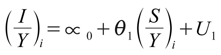
where I denotes domestic investment, S denotes national savings, Y denotes GDP, and U₁ is a random disturbance. The coefficient θ referred to as the ‘saving retention coefficient’ measures the ‘proportion of the incremental savings that is invested domestically’.

In an attempt to achieve the objective of the study, equation (1) is extended overtime and to capture variables that might help in better explaining the relationship between savings and investment and is specified as:

I N V_{i t} = α_{0} + α_{1} S A V_{i t} + α_{2} A I D_{i t} + α_{3} O P E N_{i t} + α_{4} F D_{i t} + ε_{i t}

(2)

where INV is investment as a share of GDP (INV is proxied by gross fixed capital formation), SAV denotes saving as a percentage of GDP, AID captures the proportion of foreign aid in GDP, OPEN is the degree of openness of the economy, which is measured as a ratio of GDP, and FD serves as the proxy for financial development and efficiency. The proxies are credit to the private sector as a ratio of GDP (FIN), ratio of the value of banks’ net interest margin to total assets (INTEREST) and ratio of banks’ overhead costs to real total assets (OVERHEAD). ε, i and t are the white noise disturbance term, country and time characteristics, respectively.

Data

Based on data availability, the sample size of this present study is limited to the 31 countries in SSA and for the period 1999–2011.⁴ Annual data series were sourced from World Development Indicator and International Monetary Fund databanks.

Empirical Results

This section is structured into four phases. The first phase gives a brief description of the variables employed in the model, while the second phase gives a snapshot of the unit root test results. The third and fourth phases present the cointegration and the eventual panel data estimation results, respectively.

Descriptive Statistics

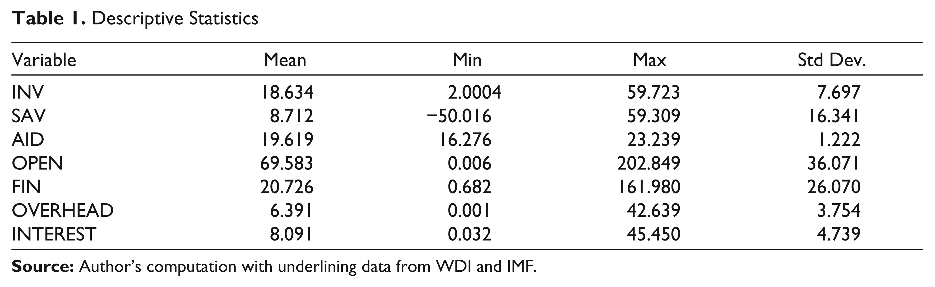
As indicated in Table 1, investment, savings and private credit have mean values of 18.63, 8.7 and 20.7 per cent, respectively. Over the same period, trade openness recorded a mean value of about 70 per cent. The positive mean values of all the variables in the model show that they are on an increasing trend. The large difference between the maximum and minimum values of all the variables (with the exception of AID, OVERHEAD and INTEREST) shows a large dispersion in the values. Finally, OPEN accounts for the largest deviation in any series, as indicated by the standard deviation.

Table 1.

Descriptive Statistics

Variable	Mean	Min	Max	Std Dev.
INV	18.634	2.0004	59.723	7.697
SAV	8.712	−50.016	59.309	16.341
AID	19.619	16.276	23.239	1.222
OPEN	69.583	0.006	202.849	36.071
FIN	20.726	0.682	161.980	26.070
OVERHEAD	6.391	0.001	42.639	3.754
INTEREST	8.091	0.032	45.450	4.739

Source: Author’s computation with underlining data from WDI and IMF.

Stationarity Test Results

The null hypothesis of no unit root at level can be rejected for all the variables using LLC and PP–Fisher chi-square. It is imperative to infer that the remaining three unit root tests produce mixed results. However, it can be summarily stated that variables that are not stationary at level become stationary when they are first differenced. These results are presented in Table 2.

Table 2.

Unit Root Test

	LLC t-stat		Breitung T-stat		IPS W-stat		ADF–Fisher Chi²		PP–Fisher Chi²
	Statistics	I(X)	Statistics	I(X)	Statistics	I(X)	Statistics	I(X)	Statistics	I(X)
INVE	−5.962(0.000)	I(0)	−1.882(0.030)	I(1)	−6.505(0.000)	I(1)	77.267(0.092)	I(0)	121.079(0.000)	I(0)
SAV	−3.159(0.000)	I(0)	−2.161(0.015)	I(1)	−1.539(0.062)	I(1)	95.442(0.004)	I(1)	100.742(0.001)	I(0)
AID	−7.088(0.000)	I(1)	−1.345(0.000)	I(1)	−6.001(0.000)	I(1)	149.137(0.000)	I(1)	361.190(0.000)	I(1)
OPEN	−5.065(0.000)	I(0)	−3.455(0.000)	I(1)	−1.624(0.053)	I(1)	79.456(0.067)	I(0)	114.120(0.000)	I(0)
FIN	−3.693(0.000)	I(0)	−1.890(0.029)	I(1)	−0.792(0.096)	I(1)	76.938(0.096)	I(1)	87.416(0.018)	I(0)
OVERHEAD	−10.912(0.000)	I(0)	−2.304(0.000)	I(1)	−3.253(0.000)	I(0)	113.861(0.000)	I(0)	174.863(0.000)	I(0)
INTEREST	−12.930(0.000)	I(0)	−1.486(0.067)	I(0)	−3.749(0.000)	I(0)	107.253(0.000)	I(0)	179.535(0.000)	I(0)

Source: Author’s computation with underlining data from WDI and IMF.

Note: LLC and IPS represent the panel unit root tests of Levin et al. (2002) and Im et al. (2003), respectively. Fisher–ADF and Fisher–PP is for Maddala and Wu (1999). Exogenous variables: individual effects and individual linear trends. Fisher test is computed using an asymptotic chi-square distribution. All other tests assume asymptotic normality.

Cointegration Test

We conducted cointegration test that was propounded by Pedroni (1999). We employ seven test approaches: panel v-statistics, panel rho-statistics, panel PP-statistics, panel ADF-statistics, group rho-statistics, group PP-statistics and group ADF-statistics. The results of these tests are presented in Table 3. Summing up, we found evidence of long-run relationships among the series in the model. Based on the foregoing, the ground is now prepared for empirical estimation of the specified model via various panel estimators, namely, OLS, FE and RE.

Table 3.

Panel Cointegration Test

Null Hypothesis: No Cointegration:	Statistics	Weighted Statistics
Alternative hypothesisCommon AR coeffs. (within-dimension)
Panel v-statistics	−3.386(0.0999)	−2.532(0.994)
Panel rho-statistics	3.497(0.999)	4.543(1.000)
Panel pp-statistics	−6.567(0.000)	−5.171(0.000)
Panel ADF-statistics	−3.457(0.036)	−3.009(0.035)
Alternate hypothesis:Individual AR coeffs. (between dimension)
Group rho-statistics	6.707(1.000)
Group PP-statistics	−9.960(0.000)
Group ADF-statistics	−4.020(0.000)

Source: Author’s computation with underlining data from WDI and IMF.

Panel Estimation Results

The retention coefficient of the pooled OLS result in Table 4 is 0.061. This coefficient remains robust to the inclusion of control variables. The addition of aid and trade openness into the model increases the savings retention coefficients from 0.061 up to 0.102. It should also be noted that the need to include these variables as important determinants of investment is demonstrated by the increase in the value of adjusted R² from 0.140 to 0.243.

This finding is in line with economic intuition. For instance, an open economy would allow for free flow of capital to wherever interest rate is high; thus, it is expected to lead to increase in investment. The positive and significant effect of aid shows its importance as a major source of foreign capital inflow in SSA. However, all the indicators of financial development (‘more finance’ and ‘better finance’) are negative determinants of investment in SSA. This is in contradiction to the belief that an efficient financial system bridges the savings–investment gap. A plausible explanation for this might be related to the improved activities of the non-official operators that are not captured by the regulators. When FIN was captured in the model, there was a slight increase in the retention coefficient up to 0.106; the inclusion of ‘better finance’, that is, INTEREST and OVERHEAD variables, considerably reduces the retention coefficients when compared to the previous models.

The inability of the pooled OLS results to explicitly account for heterogeneity in the cross sections, omitted variable bias as well as the low value of the adjusted R² lend credence to advocate for the use of better estimators. Essentially, this study considers the use of FE and RE. The study employed Hausman test to determine the model appropriateness between FE and RE. Preference is expressed in favour of FE over RE based on the level of significance of Hausman statistics.

In the FE estimates, the inclusion of AID and OPEN improved the FH coefficients. However, the inclusion of FD indicators led to decline in savings retention coefficients. This might be due to political, institutional and economic policy spheres that the least squares estimate might overlook (Adeniyi & Egwaikhide, 2012). This is similar to what is obtained in the pooled OLS results. The better performance of the FE models is further shown by the improvement in the model fit. More than 60 per cent of the variations in investment is being accounted for by the explanatory variables. Also, the exact effect of the financial development indicators is not explicitly made clear based on varying signs, magnitude and significance. The estimates of the RE models are not reported here but they are somewhat similar to that obtained in the FE models. Specifically, the retention coefficients hover between 0.047 and 0.069.

Table 4.

Estimates of Feldstein–Horioka (FH) Puzzle

	Model 1		Model 2		Model 3		Model 4		Model 5		Model 6
	OLS	FE	OLS	FE	OLS	FE	OLS	FE	OLS	FE	OLS	FE
SAV	0.061**(0.026)	0.047**(0.011)	0.064**(0.026)	0.064**(0.025)	0.102*(0.023)	0.071***(0.029)	0.106*(0.023)	0.054**(0.018)	0.070*(0.023)	0.082**(0.039)	0.082*(0.023)	0.069***(0.039)
AID			0.309(0.336)	2.206*(0.552)	2.348*(0.353)	2.023*(0.539)	2.368*(0.354)	1.741*(0.529)	2.374*(0.339)	1.991*(0.537)	2.295*(0.350)	1.940*(0.552)
OPEN					0.122*(0.012)	0.101*(0.023)	0.123*(0.012)	0.114*(0.023)	0.115*(0.011)	0.103*(0.023)	0.117*(0.012)	0.100*(0.023)
FIN							−0.013(0.013)	0.176(0.040)
OVERHEAD									−0.514*(0.089)	−0.196**(0.092)
INTEREST											−0.227**(0.075)	−0.056(0.079)
R2	0.140	0.616	0.164	0.634	0.243	0.653	0.338	0.672	0.278	0.656	0.235	0.656
Haussman Test		21.203[0.000]		18.298[0.000]		19.281[0.000]		12.025[0.000]		11.203[0.000]		14.297[0.000]

Source: Author’s computation with underlining data from WDI and IMF.

Notes: Values in parentheses are the standard errors, while *, ** and *** represent the level of statistical significance at 1%, 5% and 10%, respectively.

Overall, the saving retention coefficients obtained in this present study are not within the neighbourhood of what earlier studies reported. For instance, using pool mean group (PMG), fully modified OLS (FMOLS) and dynamic OLS (DOLS), Bangake and Eggoh (2010) found saving retention coefficients to be 0.36, 0.38 and 0.58, respectively. Adedeji and Thornton (2006) limited their study to the use of DOLS and FMOLS, and obtained the FH coefficients 0.51 and 0.73, respectively. The three studies most synonymous in spirit to ours are Payne and Kamazawa (2005), De Wet and Van Eyden (2005) and Adeniyi and Egwaikhide (2013). The obtained estimates were 0.20 (OLS), 0.23 (FE), 0.24 (RE) for Payne and Kamazawa (2005); 0.31(OLS), 0.34 (FE), 0.28 (RE) for De Wet and Van Eyden (2005); and 0.32 (OLS), 0.21 (FE), 0.24 (RE) for Adeniyi and Egwaikhide (2013).

As a preview, it can be stated that the inclusion of ‘better finance’ indicators (INTEREST and OVERHEAD) improves our FH estimates than ‘more finance’ indicator. This then suggests that improving the quality of financial services might lead to mobilization, distribution and utilization of savings for investment purposes. Hence, this should be the immediate focal point of the policy makers in the SSA region. Hence, finance seemingly matters little in the savings–investment nexus in SSA.

Table 5.

Alternative Estimates of FH Equation (interaction terms)

	1	2	3
SAV	0.049(0.050)	0.146**(0.064)	0.130**(0.061)
AID	2.153*(0.531)	2.180*(0.540)	1.956*(0.542)
OPEN	0.102*(0.023)	0.107*(0.023)	0.101*(0.023)
SAV*FIN	0.010*(0.003)
SAV*OVERHEAD		0.017**(0.007)
SAV*INTEREST			−0.006(0.005)
R²	0.667	0.680	0.656

Source: Author’s computation with underlining data from WDI and IMF.

Notes: Values in parentheses are the standard errors, while *, ** and *** represent the level of statistical significance at 1%, 5% and 10%, respectively.

In an attempt to further understand the purported role of finance (‘better finance’, ‘more finance’) in the saving–investment nexus, the study interacted finance measures with savings. This is to provide information on how finance helps create and mobilize savings for effective and productive use and as such how it affects the magnitude of saving retention coefficients. These results (FE alone) are presented in Table 5. ‘Better finance’ indicators increased FH coefficients to 0.146, while ‘more finance’ decreased our FH estimates, albeit, insignificantly. This finding serves as a new as well as an additional evidence to the existing stock of literature on FH puzzle. It is pertinent to mention that these interactive terms are positive and significant. This provides sterling evidence of how qualitative measures of financial development perform their microeconomic functions, which seek to decrease overhead cost, increase net interest margin as well as channel savings to the most productive sector. This chain of events leads to a reduction in negative net present value projects by banks.

Conclusion and Implications

Using annual data set for 31 countries in SSA and for the period from 1999 to 2011, the study revisited the FH puzzle. The novelty of this study is the inclusion of qualitative proxies (ratio of the value of banks’ net interest margin to total assets and ratio of overhead costs to real total assets) of finance in the estimated models. Results of the stationarity tests showed the stationarity of all the variables. The cointegration results established a long-run relationship among the series in the model.

The estimates of the saving retention coefficient are 0.061 (OLS), 0.047 (FE) and 0.052 (RE). These are dissimilar to the coefficients of earlier studies on FH puzzle. We found that when the traditional measure of finance was incorporated into the model, saving retention jumped significantly. This is indicative of marked effect of the traditional measure of finance in the puzzle. For instance, the FH coefficient increased from 0.061 to 0.106. This lends support to the role of finance in mobilizing savings for investment within an economy. However, when the measures of finance interacted with savings, qualitative measures of finance increased FH estimates to 0.146. This attests to the fact that qualitative measures are better proxies of financial development. Based on the foregoing, it is imperative for policy makers to design policies that would seek to improve the ‘better finance’ indicators of SSA countries so as to ensure increased effect of saving on investment and ceteris paribus economic growth.

Footnotes

Acknowledgements

The author is grateful to the anonymous referees of the journal for their extremely useful suggestions to improve the quality of the article. Usual disclaimers apply.

Notes

References

Adedeji

, & Thornton

(2006). Saving, investment and capital mobility in African countries. Journal of African Economies, 16(3), 393–405.

Adeniyi

, & Egwaikhide

F.O.

(2013). Saving-Investment Nexus In Developing Countries: Does Financial Development Matter? Journal Of Economic Development 38(2), 119–140.

Apergis

, & Tsoumas

(2009). A survey on the Feldstein–Horioka puzzle: What has been done and where we stand. Research in Economics, 63(1), 64–76.

Arestis

, & Demetriades

(1996). Finance and growth: Institutional considerations and causality. Department of Economics working paper no. 5. London: University of East London.

Bajo-Rubio

(1988). The saving–investment correlation revisited: The case of Spain 1964–1994. Applied Economics Letters, 5(12), 769–772.

Bangake

, & Eggoh

J.C.

(2010). International capital mobility in African countries: Do the legal origins matter? Economics Bulletin, 30(1), 73–83.

Beck

, Demirguc-Kunt

, & Levine

(1999). A new database on financial development and structure. World Bank Policy Research working paper 2146. Washington, DC: World Bank. (updated in 2013).

Bettin

, & Zazzaro

(2009). Remittances and financial development: Substitutes or complements in European countries (pp. 1–21). Mo.Fi.R working paper 28. Mo.Fi.R, Washington D.C.

Coakley

, Kulasi

, & Smith

(1998). The Feldstein–Horioka puzzle and capital mobility: A review. International Journal of Finance and Economics, 3(2), 169–188.

10.

Coakley

, Fuertes

A.M.

, & Spagnolo

(2004). Is the Feldstein–Horioka puzzle history? The Manchester School, 72(5), 569–590.

11.

Cooray

(2012). Migrant remittances, financial sector development and the government ownership of banks: Evidence from a group of non-OECD economies. International Financial Markets, Institution and Money, 22(4), 936–957.

12.

De Wet

A.H.

, & Van Eyden

(2005). Capital mobility in sub-Saharan Africa: A panel data approach. South African Journal of Economics, 73(1), 1–22.

13.

Demetriades

, & Andrianova

(2004). Finance and growth: What we know and what we need to know. In Goodhart

(Ed.), Financial development and economic growth: Explaining the links (pp. 38–65). Basingstoke: Palgrave Macmillan.

14.

Demirgüç-Kunt

Asli

(2008). Finance and economic development: The role of government. Policy working paper no. 3955. Washington, DC: World Bank.

15.

Feldstein

, & Horioka

(1980). Domestic saving and international capital flow. The Economic Journal, 90(358), 314–329.

16.

Fouquau

, Hurlin

, & Rabaud

(2008). The Feldstein–Horioka puzzle: A panel smooth transition regression approach. Economic Modelling, 25(2), 284–299.

17.

Gundlach

, & Sinn

(1992). Unit root tests of the current account balance: Implications for international capital mobility. Applied Economics, 24(6), 617–625.

18.

T.W.

(2003). The saving-retention coefficient and country-size: The Feldstein–Horioka puzzle reconsidered. Journal of Macroeconomics, 25(3), 387–396.

19.

K.S.

, Pesaran

M.H.

& Shin

Y.C.

(2003). Testing for Units Roots in Heterogeneous Panels. Journal of Econometrics, 115(1), 53–74.

20.

Jansen

W.J.

(1996). Estimating saving-investment correlations: Evidence for OECD countries based on an error correction model. Journal of International Money and Finance, 15(5), 749–781.

21.

Jansen

W.J.

, & Schulze

G.G.

(1996). Theory-based measurement of the saving-investment correlation with an application to Norway. Economic Inquiry, 34(1), 116–132.

22.

Kim

, Oh

K.-Y.

, & Jeong

C.W.

(2005). Panel cointegration results on international capital mobility in Asian economies. Journal of International Money and Finance, 24(1), 71–82.

23.

Law

S.H.

, & Singh

(2014). Does too much finance harm economic growth? Journal of Banking and Finance, 41(1), 36–44.

24.

Law

S.H.

, Azman-Saini

W.N.W.

, & Ibrahim

M.H.

(2013). Institutional quality thresholds and the finance–Growth nexus. Journal of Banking and Finance, 37(12), 5373–5381.

25.

Levin

, Lin

C.F.

& Chu

(2002). Unit Root Test in Panel Data: Asymptotic and Finite Sample Properties. Journal of Econometrics, 108(1), 1–24.

26.

Levine

(2005). Finance and growth: Theory and evidence. NBER, working paper no. 10766. NBER, Massachusetts, Cambridge.

27.

Maddala

G.S.

, & Wu

(1999). A Comparative Study of Unit Root Tests with Panel Data and New Simple Test. Oxford Bulletin of Economics and Statistics, 61(3), 631–652.

28.

Mastroyiannis

(2007). Current account dynamics and the Feldstein and Horioka puzzle: The case of Greece. The European Journal of Comparative Economics, 4(1), 91–99.

29.

McKinnon

R.I.

(1973). Money and capital in economic development. Washington, DC: Brooking Institution.

30.

Obstfeld

(1985). Capital mobility in the world economy: Theory and measurement. Carnegie–Rochester Conference Series in Public Policy, 24(1), 55–104.

31.

Obstfeld

, & Rogoff

(2000). The six major puzzles in international macroeconomics: Is there a common cause? NBER working paper 7777. NBER, Massachusetts, Cambridge.

32.

Özmen

(2004). Financial development, exchange rate regimes and the Feldstein–Horioka puzzle: Evidence from the MENA region (Vol. 4/18, pp. 1–16). ERC working papers in economics. Ankara, Turkey: ERC.

33.

Ozmen

, & Parmaksiz

(2003). Policy regime change and the Feldstein–Horioka puzzle: The UK evidence. Journal of Policy Modeling, 25(2), 137–149.

34.

Payne

J.E.

, & Kumazawa

(2005). Capital mobility, foreign aid, and openness: Further panel data evidence from sub-Saharan Africa. Journal of Economic and Finance, 29(1), 122–126.

35.

Pedroni

(1999). Critical values for cointegration tests in heterogeneous panels with multiple regressors. Oxford Bulletin of Economics and Statistics, 61(4), 653–670.

36.

Raheem

I.D.

(2015). Remittances, financial sector development and efficiency and growth in Africa. Indian Journal of Finance, 9(2), 25–34.

37.

Raheem

I.D.

, Adeniyi

, & Ajide

K.B.

(2016). Is There a Role for Governance in the Saving-Investment Nexus for Sub-Saharan Africa? Journal of Social and Economic Development, 18(1), 120–134.

38.

Raheem

I.D.

, & Oyinlola

M.A.

(2015). Financial development, inflation and growth in selected West African countries. Journal of Economic and Sustainable Development, 7(2), 91–99.

39.

Sarno

, & Taylor

M.P.

(1998). Exchange controls, international capital flows and saving investment correlations in the UK: An empirical investigation. Weltwirtschaftliches Archive, 134(1), 69–97.

40.

Shahbaz

, & Rahman

M.M.

(2012). The dynamic of financial development, imports, foreign direct investment and economic growth: Cointegration and causality analysis in Pakistan. Global Business Review, 13(2), 201–219.

41.

Shaw

E.S.

(1973). Financial deepening in economic growth. New York: Oxford University Press.

42.

Taylor

A.M.

(2002). A century of current account dynamics. Journal of International Money and Finance, 21(6), 725–748.

43.

Tesar

L.L.

(1991). Saving, investment and international capital flows. Journal of International Economics, 31(1), 55–78.

44.

Tripathy

, & Prahdan

R.P.

(2014). Banking sector development and economic growth in India. Global Business Review, 15(4), 767–776.

45.

Yartey

C.A.

, & Adjasi

K.A.

(2007). Stock market development in sub-Saharan Africa: Critical issues and challenges. IMF working paper, 209. Washington D.C.: IMF.