A Study on the Dynamic Behaviour of Headline Versus Core Inflation: Evidence from India

Abstract

This article attempts to understand the dynamic response of core inflation and headline inflation to macroeconomic variables in the context of India. First, core inflation is calculated using the conventional exclusion measure (excluding food and energy components) and the statistical measure (asymmetrical trimmed mean, weighted median and exponential smoothing approach) by taking the monthly Consumer Price Index y-o-y inflation data from January 2012 to June 2018. Next, the study performed the comparative analysis to understand the dynamic response of both core inflation and headline inflation to different demand and supply shocks through Structural Vector Autoregressive Technique, Impulse Response Function and the Forecast Error Variance Decomposition. The findings suggest that trimming 20 per cent of the highly volatile components from the overall inflation can serve as a better proxy for the underlying medium and long-term trend in the headline inflation. Furthermore, the comparison made between headline inflation and core inflation shows that the key drivers for core inflation is the demand-side components such as real money growth, whereas headline inflation is mostly driven by the supply-side components in the context of India. The variations in core inflation are mainly observed because of the change in monetary policy decisions, hence making core inflation an important part the policy decision making. Core inflation indicates the underlying demand pressure, which can help policymakers to set adequate key policy rates to target overall inflation.

Keywords

Core inflation headline inflation monetary policy SVAR model impulse response function forecast error variance decomposition

Introduction

Understanding inflation dynamics and maintaining economic growth has become a major challenge for central banks, especially with an objective of inflation targeting. In India, monetary policy has undergone two major developments in the macroeconomic management (a) the announcement of a new monetary policy committee as part of a new framework to focus on benchmark policy rates and target inflation at a specific level and (b) the formal declaration of inflation targeting as a new monetary policy objective, where Consumer Price Index (CPI) acts a nominal anchor to target inflation at the rate 4 per cent with a band of 2–6 per cent.

In India, headline inflation is considered as a targeted variable for determining key policy rates, yet it is often claimed in literature (Bryan & Cecchetti, 1994; Clark, 2001; Cogley, 2002; Crone et al., 2013; Detmeister, 2011; Kiley, 2008; Liu & Smith, 2014; Mehra & Reilly, 2009; Mishkin, 2007; Rich & Steindel, 2005; Rather et al., 2016; Sharma & Bicchal, 2015; Smith, 2005; Wynne, 1999; 2008) that the underlying trend of headline inflation called core inflation, which removes most volatile components from overall inflation, is likely to be the best choice for monetary policy decision making.

In the context of inflation dynamics, according to Ball and Mankiw (1995), headline inflation can be decomposed into demand-driven inflation and supply-driven inflation. Demand-driven inflation is termed as core inflation, which has a long persistent impact on headline inflation. It is generally associated with inflation expectations and demand-side components in an economy. On the other hand, supply-driven inflation arises as a result of temporary supply shocks such as volatility in agricultural products as a result of monsoon failure, an increase in external market for oil prices, or significant changes in government policies that will have a direct short-term impact on headline inflation (Donkers et al., 1983; Wynne, 1999).

The major challenge in monetary policy is to accurately forecast inflation expectations. The study by Laflèche and Armour (2006) on inflation forecasts showed that inflation consists of both persistent and transitional prices. The forecast of inflation and policy rates, taking headline inflation into account, could thus lead to a prejudice in the decision making of monetary policy due to the provisional noise of headline inflation.

In this context, Mishkin (2007) said that monetary policies have an effect on aggregate demand in an economy, so central banks should be aware of the underlying demand pressures that prevail in an economy through core inflation. Policy works with lags, though; consequently, price increases due to temporary supply shocks are themselves corrected and require no monetary policy action (Bernanke, 2007; Laflèche & Armour, 2006).

Thus, policy decisions can be effective if core inflation is used to forecast key policy rates. It eliminates all the volatile components from the headline inflation and is considered as a good underlying trend.

With regard to the relevance of core inflation to policymakers, the present study has calculated 10 different alternatives of core inflation series using both the statistical and conventional exclusion methods. The statistical methods used in this study are asymmetric trimmed mean, weighted median and exponential smoothing approach, while the exclusion method excludes the most volatile components from overall or headline inflation. The purpose of calculating different core inflation series is with an objective to identify the appropriate series, which can be defined as the best underlying trend for headline inflation.

In addition, the study conducted a comparative analysis of the dynamic responses of both core inflation and headline inflation to demand and supply shocks through structural vector autoregressive (SVAR) technique, forecast error variance decomposition (FEVD) and impulse response function (IRF). In this section, the study has separately analysed the dynamic behaviour of both core and headline inflation to different demand- and supply-side factors affecting the economy. The purpose of this analysis is to understand whether core inflation is mostly driven by demand-side or supply-side factors in Indian context. Next, the study will address the question regarding the choice of inflation measure, that is, between headline or core inflation with respect to monetary policy decision for inflation targeting in the context of India.

The remainder of the study is as follows: The introduction is followed by a literature review in Section 2. Data description and methodology for constructing core inflation, as well as econometric modelling, are explained in Section 3. Section 4 and 5 discuss the empirical findings and conclusion of the study.

Literature Survey

Core Inflation as a Persistent Measure of Headline Inflation

According to Friedman’s (1968) definition, ‘inflation is a steady and sustained increase in the general price level’. The steady growth of inflation proceeds at a more or less constant rate, while intermittent inflation proceeds by fits and starts. Steady and sustained inflation is incorporated into inflation forecasts, as it tends to be less volatile than intermittent inflation. Similarly, Laidler and Parkin (1975) defined ‘inflation is a process of continuously rising prices, or, equivalently, of a continuously falling value of money’. The definition of core inflation as a persistent component, however, reflects the tendency to describe core inflation as a trend measure of headline inflation.

In line with the concept of core inflation as the persistent components of headline inflation, Otto Eckstein (1981) had formally developed the concept of core inflation and defined it as the trend increase in the cost of living of the household due to aggregate demand pressure in the economy. Keeping in view as a persistent measure of inflation, Quah and Vahey (1995) defined core inflation as ‘… a persistent measure of headline inflation. It indicates towards the medium to long term trend in the headline measure of inflation’. According to the definition given by Quah and Vahey (1995), core inflation is considered to be medium- to long-term output-neutral. This definition eliminates the impact of supply shocks that may have a permanent impact on the price level, but no lasting impact on the inflation rate. Similarly, Roger (1998) defined the concept of core inflation as both a persistent and generalized component of the headline inflation.

Survey on Construction of Core Inflation Through Alternative Approaches

With the relevance of core inflation to policymakers, different approaches have been developed and continue to build core inflation. Initially, core inflation was calculated by excluding volatile components and the effects of changes in indirect taxes from the overall inflation rate (Donkers et al., 1983, pp. 26–30).

Although many policymakers associate ‘core inflation’ with inflation, excluding food and energy, there are arguments against this approach that the excluded items may consist of relevant information on the underlying inflation. Therefore, excluding food and energy method is not an effective measure for calculating core inflation with regard to policy perspectives.

Later, statistical measures such as trimmed mean, weighted median, moving average, exponential smoothing, HP filter, wavelet filter and common component method are most commonly used to construct core inflation. These methods are flexible to exclude the impact of different components each month, based on their extreme price movement at the specific point of time.

In the literature, statistical measures were propounded by the work of Blinder and Reis (2005), Bryan and Pike (1991), Bryan and Cecchetti (1994), Clark (2001), Cogley (2002), Marques, Neves, and Sarmento (2003), Smith (2005) and Rich and Steindel (2005). Another alternative approach to calculate core inflation is the model-based approach based on economic theory propounded in the work of Blix (1995), Fase and Folkertsma (1996) and Quah and Vahey (1995).

Bryan and Cecchetti (1994) support the significance of the statistical measure for the construction of core inflation through the weighted median method by using personal consumption expenditure for the United States, while Clark’s (2001) study favoured the trimmed mean approach. According to them, both the measure (weighted median and trimmed approach) eliminate components with significant relative price changes in a given month, with the sets of excluded components varying from month to month.

In this respect (Bodenstein, Erceg, & Guerrieri, 2008; Kiley, 2008; Mishkin, 2007), studies have suggested that statistically calculated core inflation should be less volatile and highly correlated with headline inflation in order to make an effective policy decision. However, Quah and Vahey’s (1995) study suggested that the estimated core inflation by SVAR methodology is defined to be output neutral in the medium and long run. Furthermore, Bernanke’s (2007) study suggested that monetary policy works with lags; therefore, core inflation acts as a better gauge for a forward-looking approach for the policy forecasting.

Globally, research are empirically conducted to perform the comparative analysis between the exclusion method and the statistical method. Some of the recent analysis on core inflation by Alkhareif and Barnett (2015) for Saudi Arabia show that core inflation measured through excluding food and housing/rent was more volatile and weakly correlated with headline inflation. In contrast, the statistical core inflation method is relatively more stable, less volatile and has a stronger correlation with headline inflation. Similarly, Gamber et al.’s. (2015) study had proposed a new methodology and constructed a time series analysis on disaggregated inflation data to calculate core inflation. In this aspect, Knotek and Zaman’s (2017) study also had proposed a new model for now-casting headline and core inflation, which has improved the accuracy for forecasting inflation expectations.

In India, Mohanty, Rath, and Ramaiah (2000) study calculated core inflation from Wholesale Price Index (WPI) inflation data for the period from April 1983 to March 1999 by using conventional exclusion method, trimmed mean and weighted median approach. The findings supported the trimmed mean method and suggested that 20 per cent exclusion of the highly volatile components has better predictability for the underlying trend in headline inflation. Similarly, Das, John, and Singh (2009) study had also calculated 12 different series of core inflation by using trimmed mean, weighted median, exponential smoothing method, HP filter, wavelet filter, historical exclusion and SVAR methodology. The findings show that the core inflation is less volatile when calculated by excluding ‘fuel power light and lubricant’ wavelet method and SVAR methodology. Similar approaches were incorporated in the study by Kar (2009) and Raj and Mishra (2011), where they suggested that core inflation could be used as an operational guide for monetary policy in the short term. Furthermore, Sharma and Bicchal (2015), Rather, Durai and Ramachandran (2016) and Sahu and Sharma (2018) have also built core inflation through trimmed mean approach for India.

Empirical Studies to Understand the Inflation Dynamics

Bhattacharya and Patnaik’s (2014) study analyses the monetary policy for inflation targeting framework in India by applying a semi-structural new Keynesian open economy model to anchor inflation expectations. The underlying framework is a standard new-Keynesian model with rational expectations and nominal and real rigidities with aggregate demand having a role in determining output. The framework blends into a reduced form version of the forward-looking general equilibrium model with new-Keynesian features. The findings suggest that the positive domestic aggregate demand shocks, combined with accommodating monetary policy and supply-side pressure, have led to an unanchored monetary policy. Similarly, Bhattacharya (2014) study analysed the inflation dynamics and the monetary policy transmission in Vietnam. The study considered the CPI headline inflation to be weighted on the basis of price variations of tradable and non-tradable goods. The rate of price changes for tradable goods is based on the nominal exchange rate and international tradable goods prices. By using the VAR technique, the inflation model is estimated. Short- and medium-term elastics were calculated through impulse response function based on Cholesky’s decomposition. The findings suggest that in the short run, inflation is affected by nominal effective exchange rate, whereas, in medium run, GDP growth and money supply are the principal drivers of inflation. Likewise, Rao and Goyal’s (2018) study analyses the impact of non-energy commodity and oil prices on inflation, output and real exchange rate through VECM model. The impulse response functions indicate that one standard deviation shock in commodity and oil price persists for three to eight quarters over inflation and output. These findings point towards reduction in the imports of non-energy commodity and oil imports through a series of medium- and long-term structural-cum-policy reform measures and also require the intervention by monetary authority in pursuit of inflation targeting. Similarly, the study by Ekong et al. (2015) analyses the impact of oil price shocks on Nigeria's economy for the period 1986 -2011. Based on a two-stage approach, the study has investigated the effects of demand and supply shocks in the crude oil market by using SVAR techniques. The findings of the study suggest that aggregate demand and supply of the oil products in the domestic market have significant effects on the global oil prices and response of the macroeconomic aggregates with respect to shocks in the oil supply, aggregate demand and oil-specific demand were associated with different magnitude of response with each supply shocks.

In order to understand the inflation dynamics, other studies have applied the P-star model of inflation. Kiptui’s (2013) P-star inflation model study has analysed Kenya’s economic performance from 1960 to 2011. The results that have been empirically tested showed that past inflation contributes significantly to current inflation and the domestic price gap was seen as more significant than the foreign price gap while predicting Kenya’s inflation rate.

In addition to this, the novel inflation measure called Pure Inflation Guages that disaggregates price movements with equal proportional effect on all sector prices has been estimated in a further research of inflation dynamics by Darbha and Patel (2012). The results showed that by the end of 2008–09, the WPI inflation had decreased by around 1 per cent compared with about 8 per cent in 2007–08. The decline in headline inflation in 2008–09 led the authorities to adopt a tighter policy to address corrected inflation measures against each sectors.

Data Description and Methodology

Data Description

The empirical study uses monthly time series macroeconomic data covering the sample period from January 2012 to June 2018 with (2011–12) as base year price. These time series data are taken from the Handbook of Statistics on Indian Economy, Reserve Bank of India. Combined Consumer Prices Index (CPI) y-o-y is considered as a proxy for headline inflation and also used to calculate core inflation.

Macroeconomic variables such as the Industrial Production Index (IIP) and Money Stock (M3) are considered as proxies for real output gap and real money growth, respectively. Both the macroeconomics variables (IIP and M3) have been taken into account to support demand shock on core and headline inflation.

The percentage change in the money stock adjusted for CPI headline inflation is referred to as the real money growth. On the other hand, real output gap is defined as the difference between the actual output of an economy from its potential output. The potential output is the maximum amount of goods and services, that is, the most effective economic output at full employment. The deviation of the actual output from its long-term trend (potential output) has been calculated from Hodrick–Prescott decomposition (Ahumada & Garegnani, 1999), and before calculating the output gap, seasonality components were filtered using the Census X12 method.

Additionally, for supply shock, monthly percentage change in respective price indices, that is, food and energy components of the CPI basket of commodity were taken as proxies for food¹ and fuel inflation.

Methodology

At first, core inflation was calculated using conventionally exclusion-based approaches, that is, excluding food (CPIXF) energy (CPIXE) and both food and energy together (CPIXFE) from the CPI headline inflation as well as using statistical methodology (asymmetrically trimmed mean, weighted median and exponential smoothing methods) (Figure 1).

Figure 1.

Source: The author.

Next, the study has discussed the methodology for capturing dynamic effects on core inflation and headline inflation from demand and supply shocks.

Calculation of Core Inflation

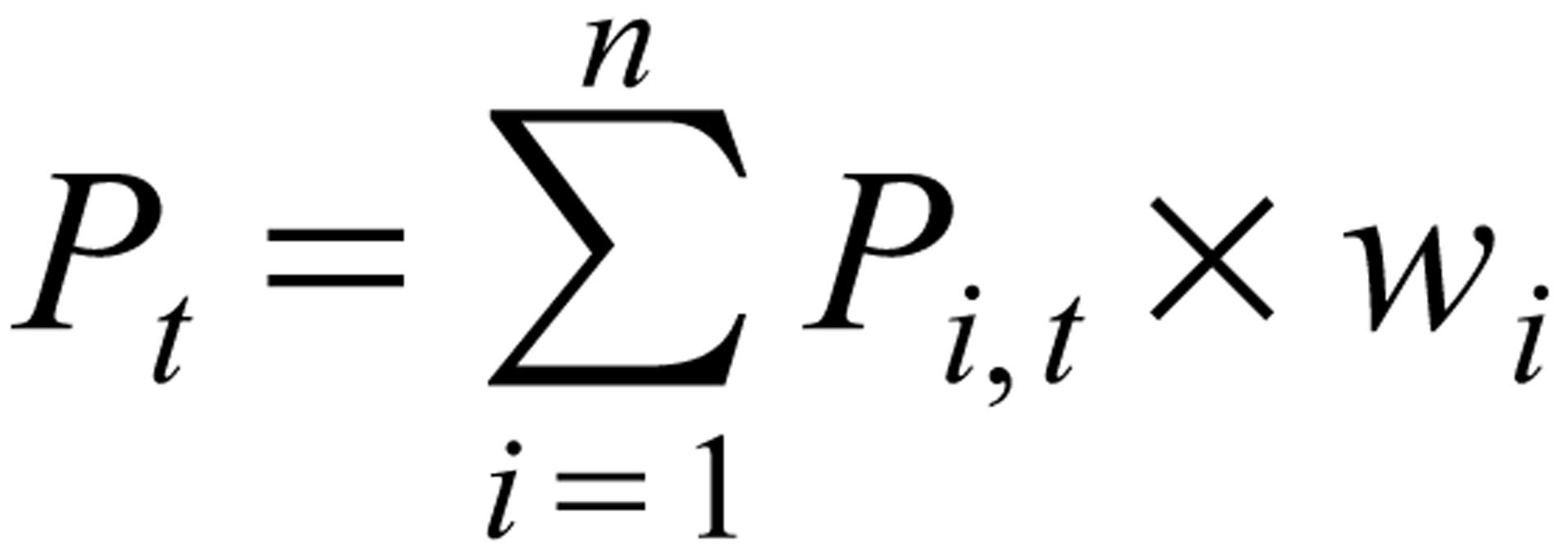
Let us consider that (p_it) is the price index of individual item (i) in period (t) and (w_i) is the weight for each commodity in the CPI basket, such that $\sum_{i =1}^{n} w_{i} =1 $ . (Here, {n} represents the number of a basic commodity in the CPI basket.)

Therefore, the aggregate price index (P_t) is as follows:

P_{t} = \sum_{i = 1}^{n} P_{i, t} \times w_{i} ​

(1)

Now, multiply the price index of each commodity with their respective weights (w_i) for calculating time-varying weights(w_it):

w_{i, t} = w_{i} \times \frac{P_{i, t}}{P_{t}} ​

(2)

Let us calculate weighted aggregate y-o-y inflation rate(π_t) as follows:

π_{i, t} = \frac{P_{i, t -} P_{i, t - 12}}{p_{i, t - 12}} ​ \times 100

(3)

π_{t} = \sum_{i = 1}^{n} π_{i, t} \times w_{i, t} ​

(4)

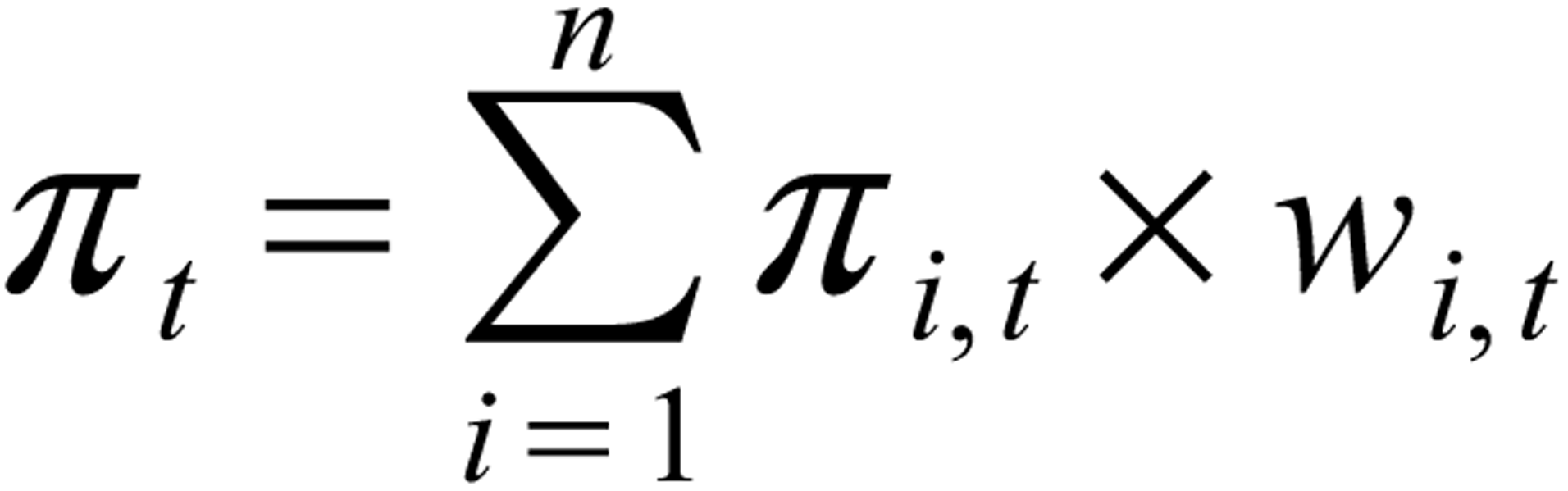
Here, (π_i,t) denotes the y-o-y inflation rate for an individual item and (π_t) represents the weighted aggregate y-o-y inflation rate of all items in the CPI basket of commodity.

Statistical Measure to Calculate Core Inflation

1. Asymmetric trimmed mean method

When data are normally distributed, symmetric trimmed mean approach is considered. On the contrary, asymmetric trimmed average approach is taken into account for the skewed distributed data.

The price distribution of data, with their respective weights in an ascending order, shall be arranged and expressed in percentile range between 1 and 100 for each month before trimming the volatile components from the CPI basket.

Now, for trimming, the centre (c) and the percentage of trim (p) are defined accordingly. The centre is defined as 50 for a symmetrical distribution of the data. However, in case of a positively skewed distribution of data, the centre exceeds 50, and it is less than 50 for a negative skewed distribution of data.

The price distribution in the present study is positively skewed, so the asymmetric trimmed mean method is used. In this, the left and right trim percentages are defined here as (L, R), where L = {(c + p – 50) and R = (c – p + 50)}.

Suppose, if the centre is set at 54 and the percentage is set at 10, then the percentile interval (L, R) as (14, 94) is determined by asymmetrically cutting the value of the price distribution, which is below 14th percentile and greater than 94th percentile, In this case, 14 per cent of the smallest price changes and 6 per cent of the largest price changes are excluded from the distribution of price data.

Likewise, if the centre is set at 50 and the trim percentage is set at 10, then the percentile interval (L, R) is given as (10, 90) which is obtained by symmetrically trimming the value of the distribution of the price below 10 per cent and more than 90 per cent. In this case, 10 per cent of the smallest and largest price distributions are symmetrically trim to calculate core inflation.

Now, the weighted average commodity prices after trimming is defined as the core inflation ((π^c) for the period (t). It takes the following form:

π_{t}^{c} = \sum_{j = 1}^{k} {w^{'}}_{j, t} \times {π^{'}}_{j, t} / \sum_{j = 1}^{k} {w^{'}}_{j, t} ​

(5)

Here, j represents the number of items in the CPI basket of commodity after trimming.

The proportion of a trim (p) is set as 10, and centre (c) is selected from 51st to 55th in this study. Thus, five core inflation alternatives are calculated by trimming 20 per cent of the volatile components by considering trimmed mean approach.

2. Weighted median and exponential smoothing method

The weighted median methodology proposed by Bryan and Cecchetti (1994) and Cogley (2002)² methodology for exponentially smoothing is used to calculate core inflation in the present study.

Conventional Exclusion-based Measure

The conventional method of exclusion excludes the most volatile elements from the CPI basket of commodity. The CPI basket contains highly volatile food and gasoline components in the short term. Only pulses and spices have shown high volatility in food and beverages components of the CPI commodity basket and are, therefore, removed from the CPI headline inflation distribution of data.

Identification of Best Measure of Core Inflation

The aim of calculating core inflation by means of different methods is to understand which core inflation measure can provide the headline inflation with a good underlying trend. The best core inflation series are identified by considering core inflation properties, as suggested in Johnson’s (1999) study: (a) Core inflation should be stable and not as volatile as headline inflation, (b) core inflation should be capable of tracking the trend of headline inflation, that is, a long-term association between headline and core inflation should be established, (c) future headline inflation should be predictable and (d) high correlation should exist between headline inflation and core inflation.

The error correction mechanism (ECM) has been applied to identify the long-term link between core inflation and headline inflation in order to select the best series from the 10 alternative series of core inflation. The ECM model takes the following form:

Δ π_{t}^{h} = \sum_{i = 1}^{n} α_{i} Δ π_{t - i}^{h} + \sum_{j = 1}^{m} β_{j} Δ π_{t - j}^{c} - y (π_{t - 1}^{h} - π_{t - 1}^{c}) + u_{t} ​

(6)

Here, (π^h) denotes headline inflation, (π^c) denotes core inflation, and u is the white noise error term. The headline and core inflation coefficients are α_i and β_j, and y is the error correction term (ECT). For headline and core inflation, the maximum number of lag values is indicated as n and m, respectively.

Headline and core inflation are both non-stationary and become stationary at first difference. The Johansen cointegration test (1991, 1995) with the use of T-Statistics and Maximum Eigenvalue has been estimated before proceeding with the ECM. The Johansen cointegration test shows significance co-integration between core and headline inflation at 1 per cent. Next, as suggested by the Akaike Information Criterion (AIC), the ECM model is estimated by three lags. The negative and significant ECT coefficient shows the long-run causality.

The root mean square error (RMSE) is then considered to know the predictive ability of core inflation. RMSE values range from 0 to 1. The lower RMSE value shows the improved forecasting strength of core inflation. Additionally, Spearman’s rank correlation test is also considered to know the correlation between headline and core inflation.

The results of the empirical analysis are shown in (Table 1). All the measures of core inflation show that the coefficient of ECT is negative and substantially significant except for CPIXE. The negative and significant ECT indicates long-term association of core and headline inflation. Furthermore, the headline inflation, as indicated by Spearman’s rank, is highly correlated to all core inflation series.

Table 1.

Best Measure of Core Inflation

Core Inflation	ECT	Standard Error	T- statistics	RMSE	Spearman’s Rank Correlation
Conventional Exclusion Method
CPI excluding food	–0.147	0.077	–1.905	1.401	0.877
CPI excluding energy	0.311	0.242	1.286	1.221	0.881
CPI excluding food and energy	–0.132	0.078	–1.687	1.463	0.883
Statistical Method
CPI weighted median	–0.256	0.089	–2.876	0.487	0.872
CPI exponential smoothing	–0.098	0.085	–1.153	0.845	0.895
Asymmetric trimmed mean
CPI(51, 10)	–0.296	0.087	–3.402	0.232	0.895
CPI(52, 10)	–0.292	0.074	–3.946	0.229	0.976
CPI(53, 10)*	–0.298	0.077	–3.870	0.219*	0.982*
CPI(54, 10)	–0.345	0.067	–5.149	0.281	0.911
CPI(55,10)	–0.217	0.088	–2.614	0.278	0.903

Source: The author.

Note: “*” indicates that the trimmed series (53, 10) has the greater predictability for headline inflation and also has the highest correlation.

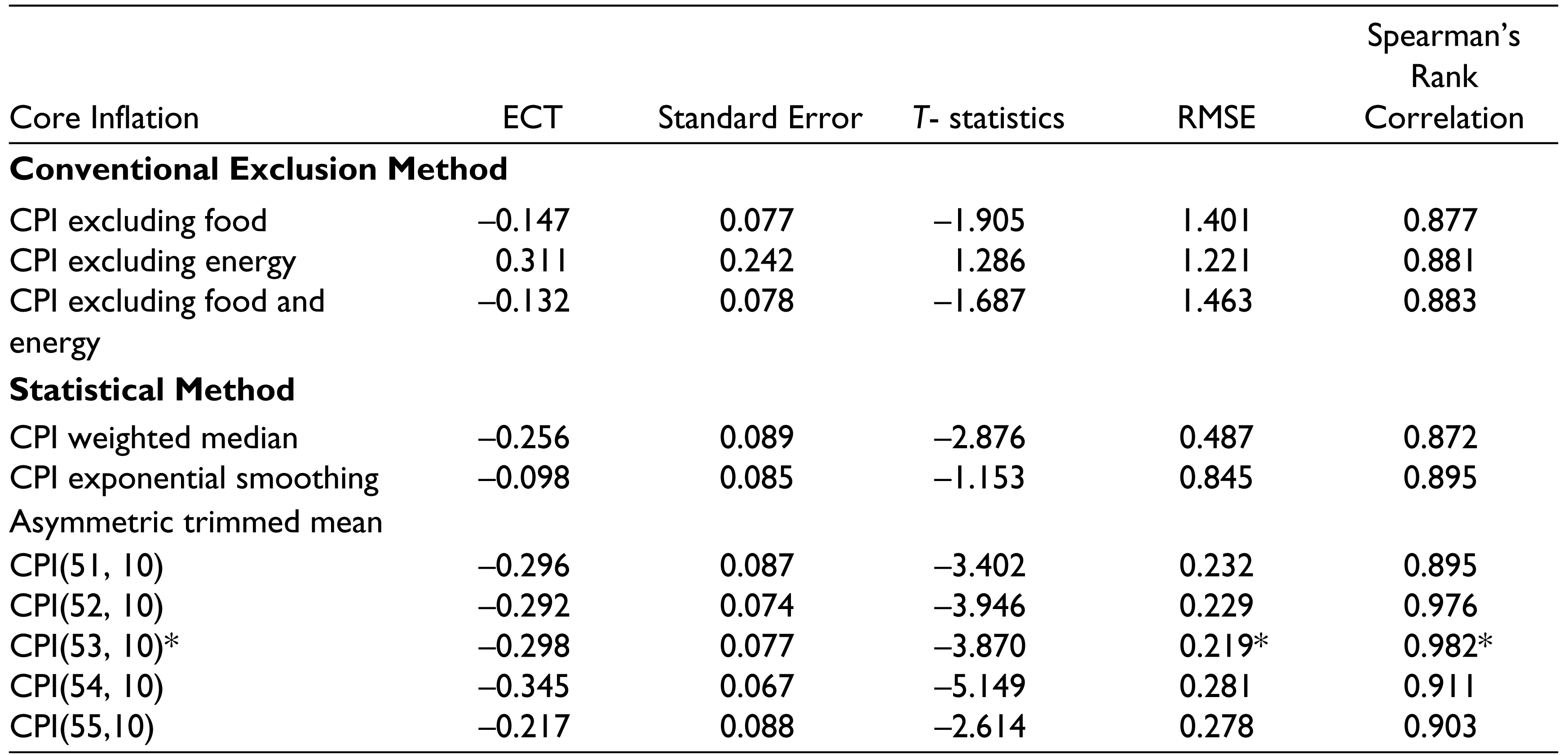
While considering for the predictive ability, it is observed that the estimated RMSE for conventional exclusion-based measures, that is, CPIXF, CPIXE and CPIXFE are more than one and show that such core inflation measures do not strongly forecast future headline inflation. The RMSE, on the other hand, has performed well and is less than one for statistical measures. Although the RMSE for trimmed series (53, 10) is better than the rest of the series, it has a strong correlation to headline inflation. Therefore, our analysis suggests (53, 10) trimmed series calculated from the asymmetrical trimmed mean approach is regarded as the best series, which can also be seen as a good trend for headline inflation. The strong correlation (0.982) with headline inflation has also been shown. Therefore, 20 per cent of trimming from the headline inflation explains better the underlying inflation trend in this study. Conversely, the conventional core inflation measures based on exclusion, that is, CPIXF, CPIXE and CPIXFE have not performed well in the current study. For the rest of the analysis (53, 10), trimmed series will be considered a measure of core inflation to understand the dynamic response of demand and supply shocks.

Core inflation as a persistent measure for headline inflation

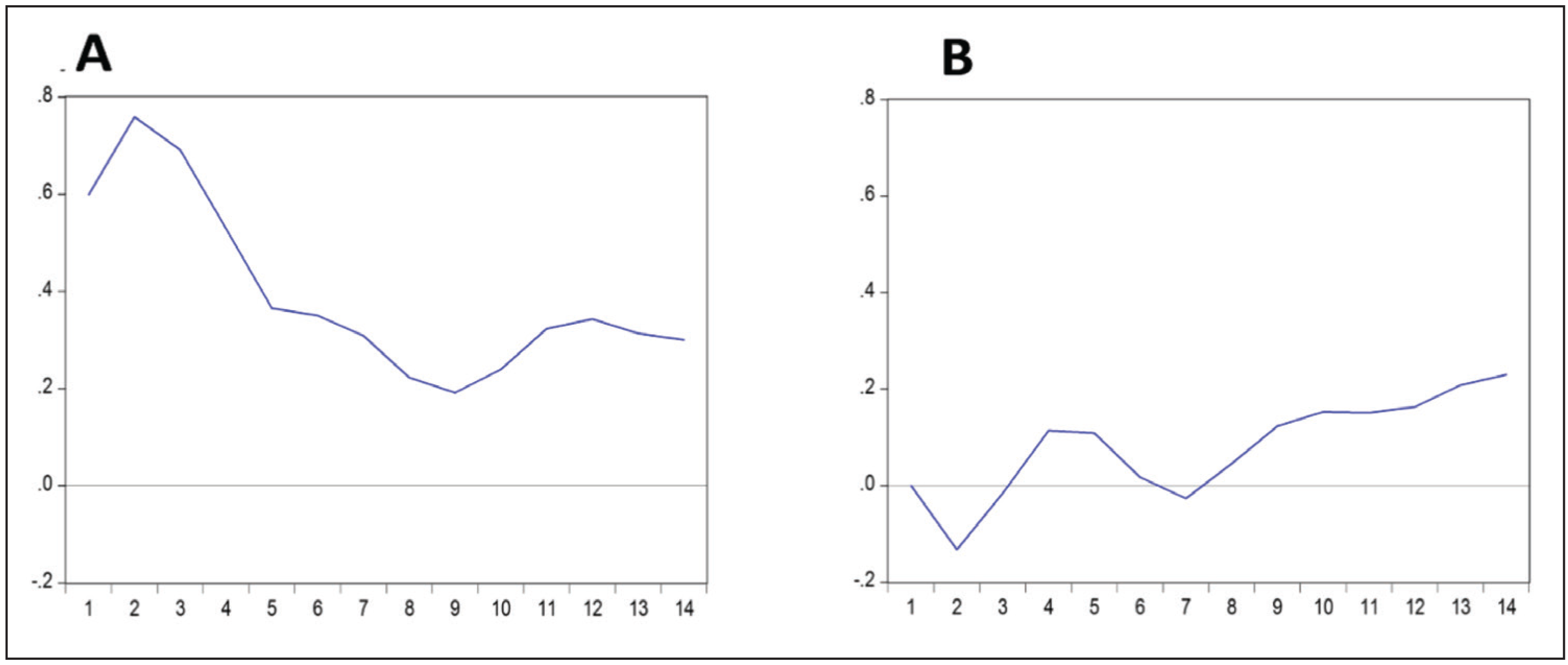
As demonstrated in Eq.6, the long run co-integration between headline and core inflation is calculated by VECM model and IRF. Taking into account the persistent measure of headline inflation, the calculated core inflation series (53, 10) is used to determine the underlying inflation trend. The response of headline inflation is observed by giving one standard deviation shock to core inflation based on Cholesky’s Decomposition.

In view of the persistent characteristics of core inflation, a long-term impact on the headline inflation was observed by giving one standard deviation shock to core inflation. However, core inflation does not seem to rise up the headline inflation in the short run, but has shown the increasing trend on the headline inflation in the long run because of economic demand pressure (Figure 2).

Figure 2.

Source: The author.

Model Specification and Theoretical Framework

Ball and Mankiw’s work (1995) can be understood in terms of theoretical modelling for core and head- line inflation, where aggregate inflation can be decomposed into demand-driven inflation and supply-driven inflation. Demand-led inflation can be linked with expected inflation and the output gap, based on the Phillips Curve (Friedman, 1968; Phelps, 1967), in which expectations are adapted. It takes the following form:

π_{t}^{D} = π_{t}^{e} + Δ y_{t} ​

(7)

Here, $(π_{t}^{D}) $ indicates demand-driven inflation, the expected inflation is denoted as $(π_{t}^{e}) $ and (πy_t) denotes output gap defined as the deviation of the actual output from the potential output.

The above specification indicates when actual output is greater than potential output, then it causes inflationary pressure and demand-pull inflation in the economy. Now, the aggregate inflation is the summation of both demand-driven inflation and supply-driven inflation. It is an extension of the expectations-augmented Phillips curve by including supply shocks (Gordon, 1977, 1982). It takes the following form:

π_{t} = π_{t}^{D} + π_{t}^{S} ​

(8)

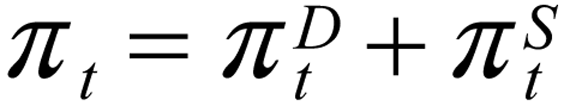
Here, (π_t) denotes the aggregate inflation and $(π_{t}^{S}) $ denotes the supply shocks or the supply-driven inflation.

Similarly, the short-run fluctuations in inflation can be understood from the P-Star approach given by Hallman, Porter, and Small (1991). It is based on the traditional quantity theory of money, that is, (MV = PT). This approach explains short-term fluctuations in aggregate inflation through the determinants of long-term equilibrium prices such as money supply, potential output and the velocity of money. The fluctuations in the aggregate inflation—high, low and remain unchanged—will depend upon whether actual price is below, above, or equal to long-run equilibrium prices.

Based on theoretical understanding, the study framed two models in order to comprehend the inflation dynamics. In Model 1, the dynamic impact on core inflation and in Model 2, the dynamic impact on headline inflation is explained. The dynamic effect of demand and supply shocks on either inflation are understood through Structural Vector Auto Regressive (SVAR), forecast error variance decomposition (FEVD) and impulse response function (IRF).

Econometric Modelling

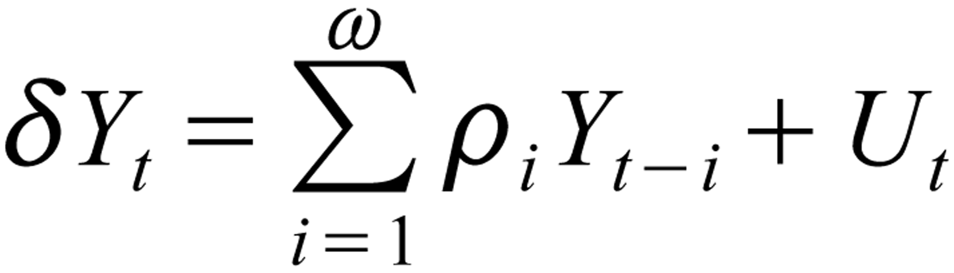
The SVAR (ω) has the following specification:

δ Y_{t} = \sum_{i = 1}^{ω} ρ_{i} Y_{t - i} + U_{t} ​

(9)

Let us take into consideration the following:

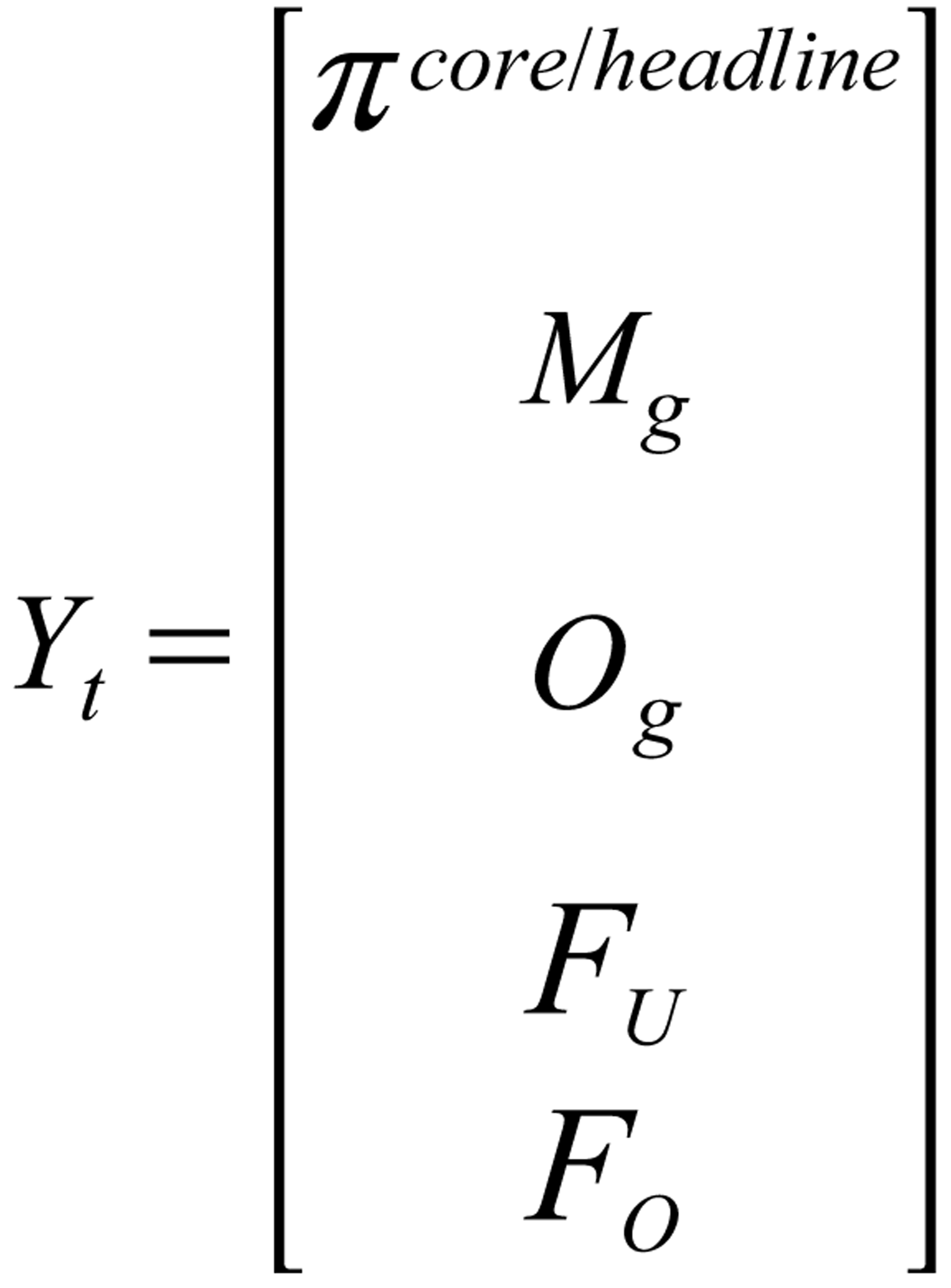
Y_{t} = [\begin{matrix} π^{c o r e / h e a d l i n e} \\ M_{g} \\ O_{g} \\ \begin{matrix} F_{U} \\ F_{O} \end{matrix} \end{matrix}] ​

Here, (Y_t) is the endogenous vector that consists of core and headline inflation (π), real production gap (O_g), real money growth (M_g) and seasonally adjusted food inflation (fo) and fuel inflation(fu).

The orthonormal unobserved structural innovation with a white noise is referred as (U_t).

(δ) indicates the (n × n) matrices of the endogenous variables, the structural coefficients that captures the dynamic interactions between the variables included in the model are indicated as ρ_1…ρ_ω and the lag operator is denoted as (ω).

Now, reduced form equation of the structural form system is estimated by pre-multiplying equation (9) with δ^–1, which is described as follows:

Y_{t} = \sum_{i = 1}^{ω} \forall_{i} Y_{t - i} + ε_{t} ​

(10)

Here, ∀_i = ρ_iδ^–1 is the reduced form lag matrix of the coefficients and ε_t = δ^–1U_t is the innovation or shock of the reduced form equation with a white noise process, and the structural variance-covariance matrix is a diagonal matrix normalized to an identity matrix. The SVAR model is useful for identifying structural shocks relevant to economic interpretation, and it is important that the system of equations should impose appropriate restrictions. The following vector is given with five endogenous variables; the VAR order is taken as supply shocks, followed by shock on demand and inflation:

(F_U → F_O → M_g → O_g → π).

The order of the variables assumes the following restriction:

U_t = ε_t

[\begin{matrix} 1 \\ 0 \\ 0 \\ \begin{matrix} 0 \\ 0 \end{matrix} \end{matrix} \begin{matrix} 0 \\ 1 \\ 0 \\ \begin{matrix} 0 \\ 0 \end{matrix} \end{matrix} \begin{matrix} 0 \\ 0 \\ 1 \\ \begin{matrix} 0 \\ 0 \end{matrix} \end{matrix} \begin{matrix} 0 \end{matrix}] [\begin{matrix} 0 \\ 0 \\ \begin{matrix} 1 \\ 0 \end{matrix} \end{matrix} \begin{matrix} 0 \\ 0 \\ 0 \\ \begin{matrix} 0 \\ 1 \end{matrix} \end{matrix}] ​ [\begin{matrix} U^{F_{U}} \\ U^{F_{O}} \\ U^{M_{g}} \\ \begin{matrix} U^{O_{g}} \end{matrix} \end{matrix}] \begin{matrix} U^{π} \end{matrix} = [\begin{matrix} a_{F_{U}}^{F_{U}} \\ a_{F_{U}}^{F_{O}} \\ a_{F_{U}}^{M_{g}} \\ \begin{matrix} a_{F_{U}}^{O_{g}} \\ a_{F_{U}}^{π} \end{matrix} \end{matrix} \begin{matrix} 0 \\ a_{F_{O}}^{F_{O}} \end{matrix}] [\begin{matrix} 0 \\ \begin{matrix} a_{F_{O}}^{O_{g}} \\ a_{F_{O}}^{π} \end{matrix} \end{matrix} \begin{matrix} 0 \\ 0 \\ a_{M_{g}}^{M_{g}} \\ \begin{matrix} a_{M_{g}}^{O_{g}} \\ a_{M_{g}}^{π} \end{matrix} \end{matrix} \begin{matrix} 0 \\ 0 \\ 0 \\ \begin{matrix} a_{O g}^{O_{g}} \\ a_{O_{g}}^{π} \end{matrix} \end{matrix} \begin{matrix} 0 \\ 0 \\ 0 \\ \begin{matrix} 0 \end{matrix} \end{matrix}] \begin{matrix} a_{π}^{π} \end{matrix} [\begin{matrix} ε^{F_{U}} \\ ε^{F_{U}} \\ ε^{M_{g}} \\ \begin{matrix} ε^{o_{g}} \\ ε^{π} \end{matrix} \end{matrix}] [\begin{matrix} 1 \\ 0 \\ 0 \\ \begin{matrix} 0 \\ 0 \end{matrix} \end{matrix} \begin{matrix} 0 \\ 1 \end{matrix}] [\begin{matrix} 0 \\ \begin{matrix} 0 \\ 0 \end{matrix} \end{matrix} \begin{matrix} 0 \\ 0 \\ 1 \\ \begin{matrix} 0 \\ 0 \end{matrix} \end{matrix} \begin{matrix} 0 \\ 0 \\ 0 \\ \begin{matrix} 1 \\ 0 \end{matrix} \end{matrix} \begin{matrix} 0 \\ 0 \\ 0 \\ \begin{matrix} 0 \\ 1 \end{matrix} \end{matrix}] ​ [\begin{matrix} U^{F_{U}} \\ U^{F_{O}} \\ U^{M_{g}} \\ \begin{matrix} U^{O_{g}} \\ U^{π} \end{matrix} \end{matrix}] = [\begin{matrix} a_{F_{U}}^{F_{U}} \\ a_{F_{U}}^{F_{O}} \end{matrix}] [\begin{matrix} a_{F_{U}}^{M_{g}} \\ \begin{matrix} a_{F_{U}}^{O_{g}} \\ a_{F_{U}}^{π} \end{matrix} \end{matrix} \begin{matrix} 0 \\ a_{F_{O}}^{F_{O}} \\ 0 \\ \begin{matrix} a_{F_{O}}^{O_{g}} \\ a_{F_{O}}^{π} \end{matrix} \end{matrix} \begin{matrix} 0 \\ 0 \\ a_{M_{g}}^{M_{g}} \\ \begin{matrix} a_{M_{g}}^{O_{g}} \\ a_{M_{g}}^{π} \end{matrix} \end{matrix} \begin{matrix} 0 \\ 0 \\ 0 \\ \begin{matrix} a_{O g}^{O_{g}} \\ a_{O_{g}}^{π} \end{matrix} \end{matrix} \begin{matrix} 0 \\ 0 \\ 0 \\ \begin{matrix} 0 \\ a_{π}^{π} \end{matrix} \end{matrix}] [\begin{matrix} ε^{F_{U}} \\ ε^{F_{U}} \\ ε^{M_{g}} \\ \begin{matrix} ε^{o_{g}} \\ ε^{π} \end{matrix} \end{matrix}]

The restrictions imposed show that the rise in oil prices due to foreign markets will influence domestic variables. The immediate consequences of the rise in oil prices will have an inflationary impact on food prices leading to cost-push inflation. This temporary shock will increase the headline inflation rate. Next, a contractionary monetary policy decision to control inflation will increase the cost of investment in the short period and thereby affects the growth of output with a lag. The effects of such a contractionary monetary policy may lead to a rise in demand-pull inflation or core inflation, thus further causing overall inflation to rise. Additionally, the endogenous variables are also affected by their own lags values. Two lag values are selected for each variable as suggested by the lag selection criteria method (Schwarz Information Criteria).

Empirical Findings and Discussions

In order to check the stationarity of the variables, augmented Dickey–Fuller test and the Phillips–Peron unit root tests are performed. The unit root test results show that the variables are integrated of order one, that is, they become stationary at the first difference.

Next, the long-term co-integration relationship between core inflation and demand-supply side components is then examined with application of Johansen’s co-integration tests (1991, 1995)³ based on Trace Statistics and Maximum Eigen value. In view of the fact that the variables are non-stationary at level, it was observed that they do not cointegrated in the long run. The same goes for Model 2 with headline inflation (Tables 2 and 3).

Table 2.

Unit root test

Variables	ADF Test		PP Test
Variables	With Intercept	With Intercept and Trend	With Intercept	With Intercept and Trend
Core inflation	0.261	0.233	0.103	0.161
Headline inflation	0.219	0.912	0.880	0.219
Real output	0.697	0.675	0.189	0.166
Real money	0.709	0.181	0.181	0.627
Fuel inflation	0.522	0.176	0.231	0.647
Food inflation	0.356	0.345	0.656	0.342

Source: The author.

Notes: Figures denote the p value at level. All the variables are non-stationary at level and become stationary at first difference. At first difference, the p value are significant at one percent level of significance.

Table 3a.

Johansen Cointegration Test (Rank Test)

Model 1. Dependent Variable: Core Inflation
Number of Cointegration	Trace Statistics				Maximum Eigenvalue
Number of Cointegration	Eigen value	Trace Statistic	Critical Value	P-value	Maximum Eigenvalue Statistic	Critical Value	P-value
None*	0.33	29.64	33.87	0.14	43.03	47.85	0.13
At most 1	0.24	20.23	27.58	0.36	27.79	32.12	0.18
At most 2	0.22	18.45	21.13	0.11	22.79	29.81	0.25

Source: The author.

Notes: “*” denotes rejection of the null hypothesis at the 0.05 level.

Trace test indicates no cointegration at the 0.05 level.

Max-eigenvalue test indicates no cointegration at the 0.05 level.

Table 3b.

Johansen Cointegration Test (Rank Test)

Model 2. Dependent Variable: Headline Inflation
Number of Cointegration	Trace statistics				Maximum Eigen value
Number of Cointegration	Eigenvalue	Trace Statistic	Critical Value	P-value	Maximum Eigenvalue Statistic	Critical Value	P-value
None*	0.32	47.84	50.48	0.15	28.55	33.87	0.18
At most 1	0.26	28.49	29.81	0.24	22.01	27.58	0.22
At most 2	0.21	19.13	23.84	0.29	17.64	21.13	0.14

Source: The author.

Notes: “*” denotes no rejection of the hypothesis at the 0.05 level.

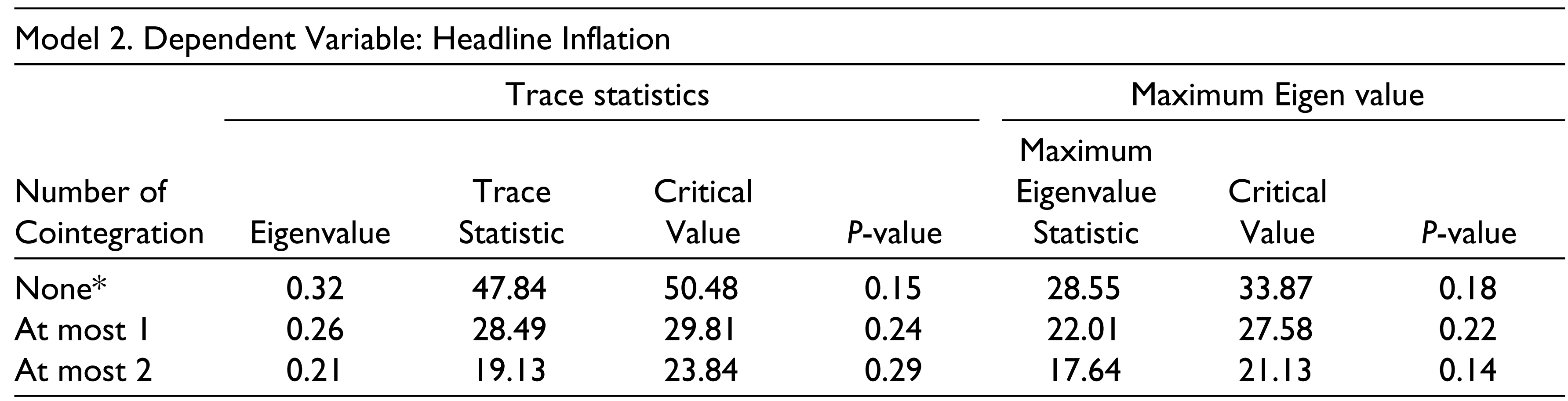
Trace test indicates no cointegration at the 0.05 level.

Max-eigenvalue test indicates no cointegration at the 0.05 level.

Since variables in both models are non-stationary and also not cointegrated in the long run, the study, therefore, took into account the SVAR technique in order to understand the dynamics of inflation. The study conducted the SVAR technique, taking into account the first difference of the variables for both models.

Inflation’s Short-run Dynamics

The estimated coefficients of the inflation models are represented in (Table 4).

Table 4.

Estimated Coefficients of the Inflation Model

Variables	Model 1 Dependent Variable Core Inflation			Model 2 Dependent Variable Headline Inflation
Variables	Coefficient	Std Error	T-statistics	Coefficient	Std Error	T-statistics
$π_{t - 1}^{h} $				0.316	0.098	3.226*
$π_{t - 2}^{h} $				0.242	0.095	2.547*
$π_{t - 1}^{c} $	0.212	0.069	3.045*
$π_{t - 2}^{c} $	0.103	0.051	2.002*
$F_{U_{t - 1}} $	0.124	0.084	1.476**	0.245	0.087	2.816*
$F_{U_{t - 2}} $	0.083	0.075	1.107**	0.197	0.067	2.940*
$v$	0.249	0.097	2.562*	0.273	0.094	2.904*
$F_{O_{t - 2}} $	0.174	0.097	1.794**	0.228	0.087	4.071***
$O g_{t - 1}$	0.084	0.019	4.421***	0.034	0.012	2.833*
$O_{g_{t - 2}} $	0.052	0.014	3.714**	0.023	0.017	1.353**
$M_{g_{t - 1}} $	0.211	0.093	2.269*	0.087	0.034	2.558*
$M_{g_{t - 2}} $	0.152	0.054	2.815*	0.073	0.045	1.622**
Constant	0.198	0.186	1.065**	0.372	0.249	1.494**

Source: The author.

Notes: 1. Model 1. Adjusted R square = 0.31 and Root Mean Square Error = 0.44.

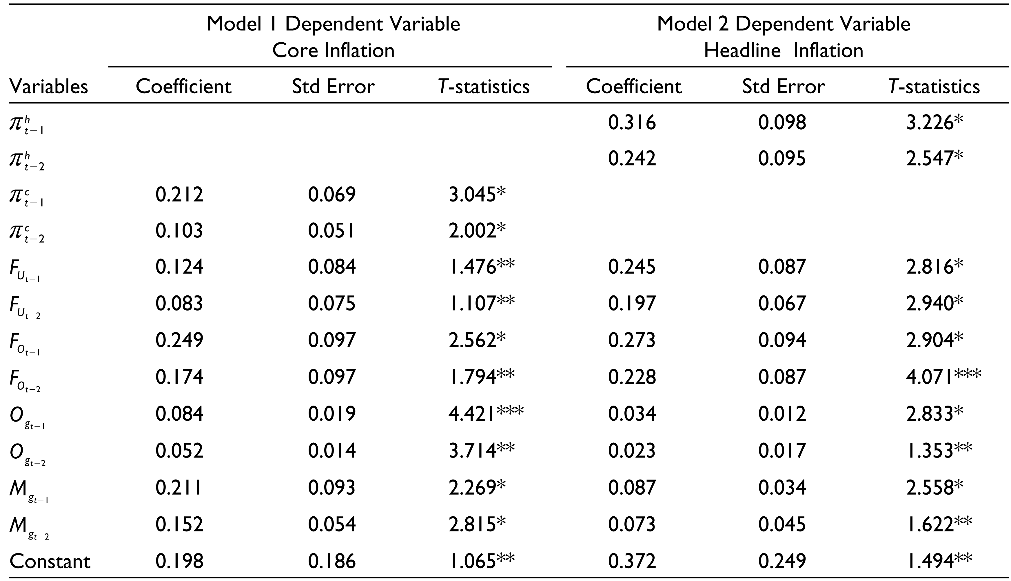
2. Model 2. Adjusted R square = 0.32 and Root Mean Square Error = 0.43.

3. ***, *, ** denote 1, 5 and 10 percent level of significance.

The estimated coefficients of core inflation as a dependent variable are represented in Model 1. Likewise, the estimated headline inflation coefficients are represented by Model 2.

The results of the estimated coefficients show that demand-side and supply-side components have a positive effect on both core inflation and headline inflation. It is apparent that core inflation and headline inflation are positively influenced by their own lags at 5 per cent significance level. In addition, the impact of lagged food and fuel inflation (F_U, F_O) taken as the proxy for supply shocks have also shown the significant positive effect on both the inflation measures. However, in relation to headline inflation, the magnitude of the estimated coefficient value is higher when it comes to supply shocks.

In contrast to this, the impact of real money growth (M_g) and real output gap (O_g) taken as the proxy for demand shocks have also shown the positive impact on both the inflation measures, but the magnitude of the estimated coefficients is greater in relation to the core inflation. It is interesting to note, therefore, that the real variables, especially, the real money growth explains core inflation more persistently than headline inflation.

Evidence from the Impulse Response Function

This section discusses the dynamic response of the inflation measures estimated over a period of 14 months by giving one standard deviation shock to the macroeconomic variables based on Cholesky’s Decomposition. The order of the SVAR is as follows: supply shocks followed by demand shocks and the inflation.

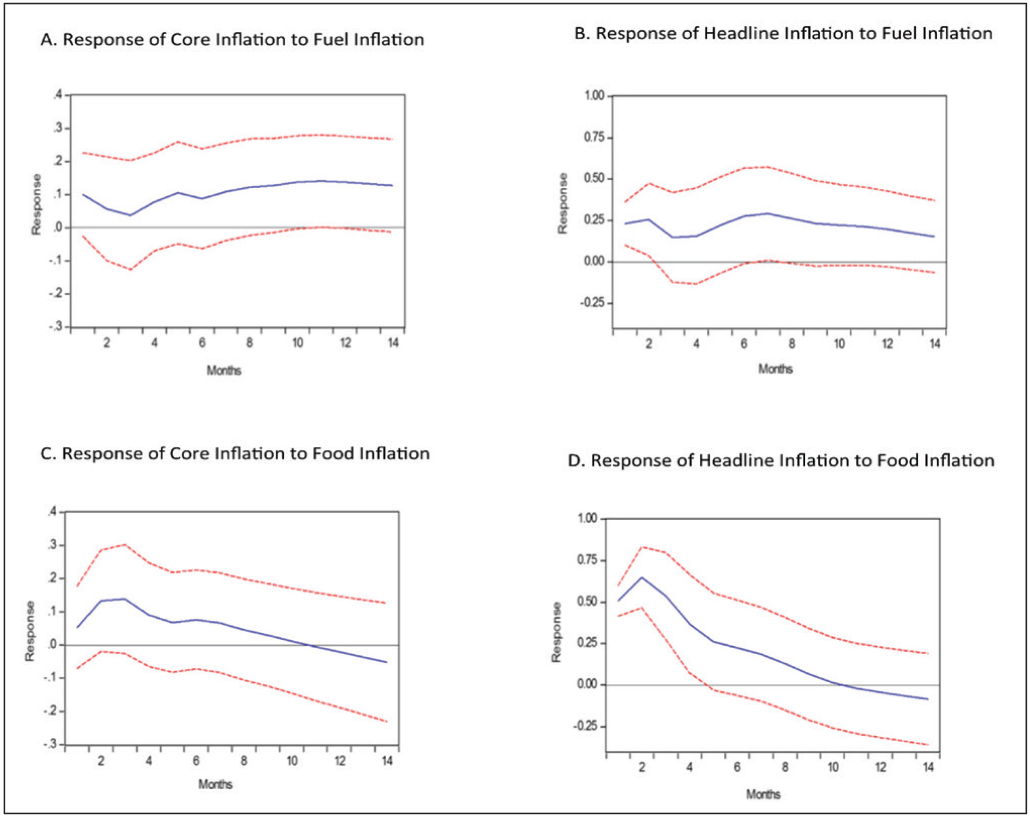
1. Inflation dynamics with respect to supply shocks

As far as fuel inflation shock is concerned, core inflation and headline inflation are instantly increasing by approximately 0.1 per cent and by 0.25 per cent while the food inflation shock raises core inflation by 0.15 per cent and headline inflation by 0.65 per cent after a month. In addition, both core inflation and headline inflation have shown a transitory response to fuel inflation and remain positive during the months, while the immediate positive effects of food inflation on both core and headline inflation remain up to 2 months and then start to decrease In fact, the IRF observation shows that the headline inflation response to supply shocks is more responsive than core inflation and is mainly driven by supply-side factors in the economy (Figure 3).

Figure 3.

Source: The author.

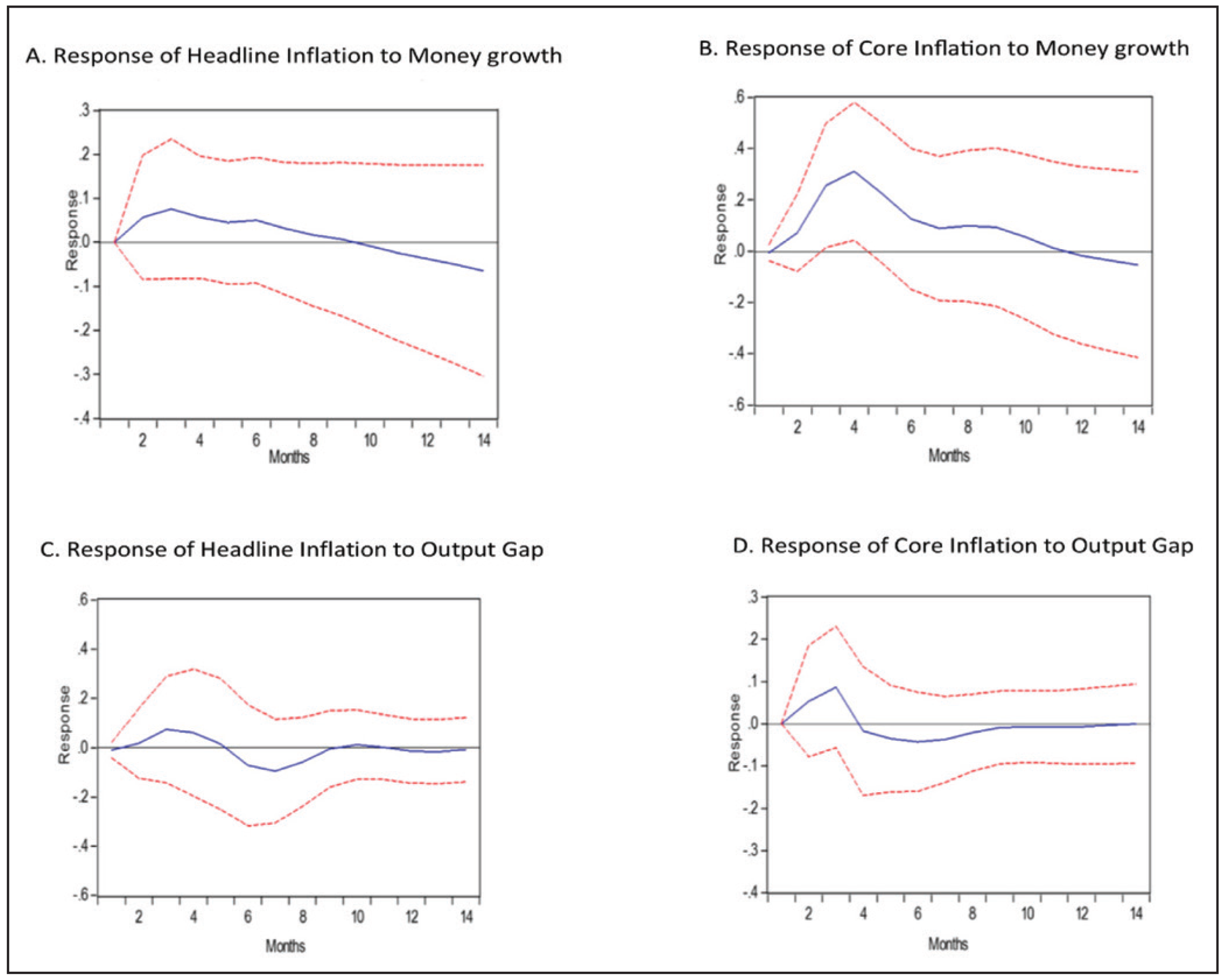
2. Inflation dynamics with respect to demand shocks

In terms of demand shocks, headline inflation is increased approximately 0.05 per cent by a real money shock and 0.09 per cnet by a real output gap shock. Shocks effects can be observed for up to 3 months and then begins to decline. Likewise, by giving one standard deviation shock to of real money growth and real output gaps, core inflation is also seen to rise by 0.3 and 0.09 per cent for up to 4 months and then declines.

It is, therefore, interesting to note that both core and headline inflation indicates output neutrality in the long run, that is, there is no long-term impact of output gap on core inflation. The impact of demand shocks can only be observed up to 4 months in case of real output gap. Another interesting note is that in the event of real monetary growth, the response of core inflation is increased. This shows that monetary policy decisions affect core inflation much more than headline inflation, which makes core inflation a major component. Therefore, it is important to note that core inflation information can be used as an instrument to understand the underlying demand pressure in the economy, which can help policymakers to set relevant policy rates for controlling overall inflation (Figure 4).

Figure 4.

Source: The author.

Forecast Error Variance Decomposition

FEVD is estimated for the period of 14 months for both core inflation and inflation. After 14 months, the dependent variable is not much varied because of various shocks taken into account in the analysis (Table 5).

Table 5.

Forecast Error Variance Decomposition (FEVD)

Period	Model 1 Dependent Variable Core Inflation π^c					Model 2 Dependent Variable Headline Inflation π^h
Period	F_U	F_O	M_g	O_g	π^c	F_U	F_O	M_g	O_g	π^h
1	1.12	0.33	2.22	1.28	94.81	15.21	75.85	0.03	0.01	12.91
2	1.21	1.51	2.64	1.21	88.70	12.87	80.87	0.21	0.72	13.85
3	1.47	2.77	2.56	2.25	82.32	10.03	75.49	1.86	1.57	11.52
6	4.57	4.78	4.91	2.57	77.15	15.42	59.75	1.81	1.61	11.45
7	5.53	4.88	5.60	2.22	75.40	18.00	57.34	1.45	1.59	10.36
8	7.23	4.94	5.14	1.82	74.17	19.98	55.33	1.36	1.51	9.51
11	7.93	4.64	6.82	1.65	72.36	24.61	49.13	1.28	1.26	8.32
12	7.82	4.42	6.54	1.64	72.02	25.54	47.44	1.23	1.21	8.55
14	7.49	4.21	6.36	1.61	71.80	26.15	46.00	1.24	1.14	8.81

Source: Author’s Calculations.

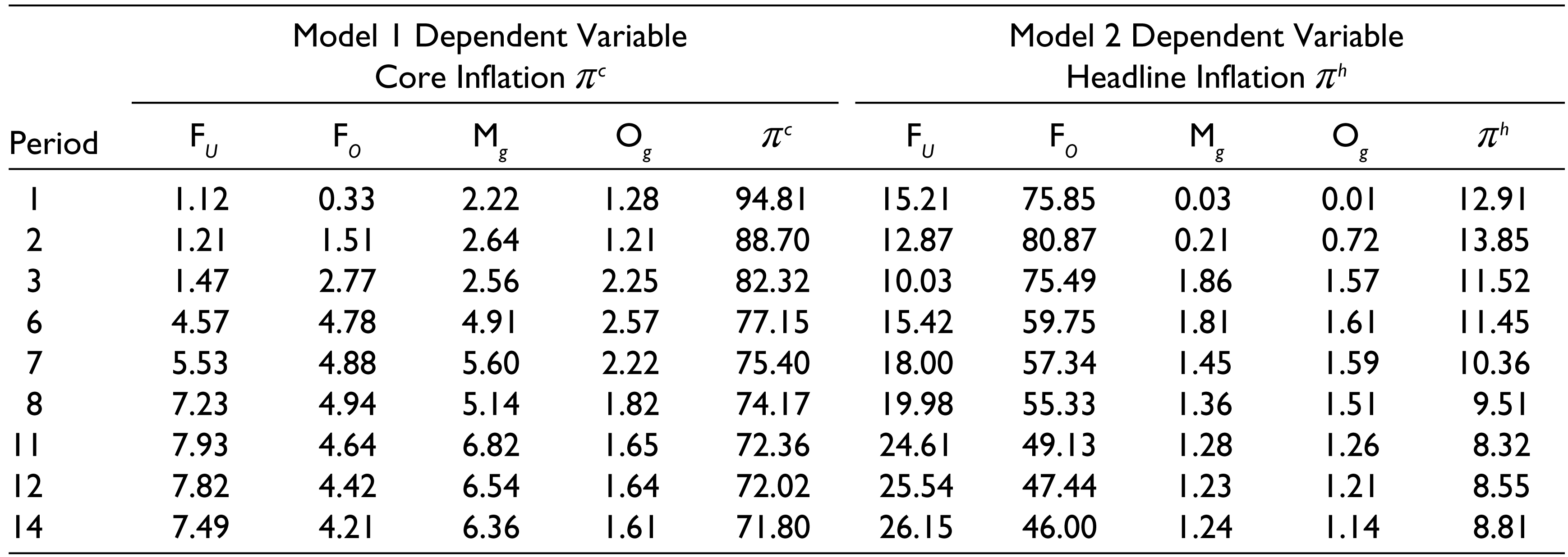
In view of Model 1, considering core inflation as a dependent variable, 95 per cent of the core inflation variations were due to its own lags, followed by real money growth (2.22%) and output gap (1.28%), fuel inflation (1.12%) and food inflation (0.33%). It is also apparent that long-term impact in the core inflation caused by real money growth, output gap and fuel inflation can be observed up to 8 to 11 months, and beyond that, there is not much variations. In contrast, food inflation has an impact on core inflation up to 3 to 6 months, and beyond that, it starts to decline, suggesting that food inflation has no long-term effect on core inflation. Likewise, it is clear in Model 2 that variation in headline inflation is mostly explained through food inflation (76%), followed by fuel inflation (15%), real money growth (0.03%) and real output gap (0.01%).

Therefore, the analysis carried out confirms that the real variables affect core inflation more. The immediate effect of demand shocks in core inflation is promptly observed, and real money growth continues to have a persistent impact on core inflation, which makes it useful in making monetary policy decisions. Contrary to this, variation explained by supply shocks is high in case of headline inflation compared with the core inflation, suggesting that headline inflation in India is mostly driven by supply-side factors in the economy.

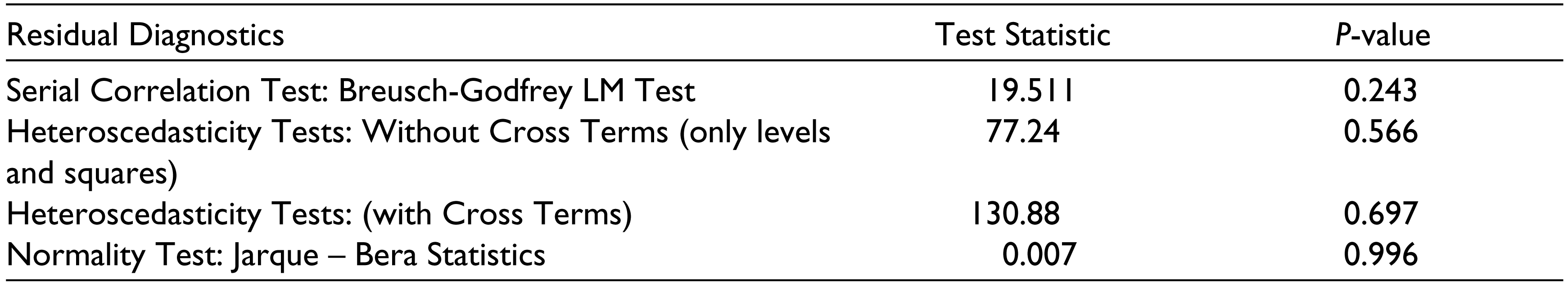
Residual Diagnostic

To test the presence of serial correlation in the residuals, Breusch–Godfrey Lagrange Multiplier tests based on F-statistics is considered. The null hypothesis of no serial correlation cannot be rejected at 5 per cent level of significance at lag one. Next, to test the presence of heteroscedastic, White’s Heteroscedasticity Test with cross product of the regressors, as well as the levels and the square values of the regressors based on Chi-square distribution, is used. Again, we cannot reject the null hypothesis of homoscedasticity residuals at 5 per cent level of significance, and Jarque-Bera Statistics indicates that the residuals are normally distributed (Table 6).

Table 6.

Residual Diagnostic Test

Residual Diagnostics	Test Statistic	P-value
Serial Correlation Test: Breusch-Godfrey LM Test	19.511	0.243
Heteroscedasticity Tests: Without Cross Terms (only levels and squares)	77.24	0.566
Heteroscedasticity Tests: (with Cross Terms)	130.88	0.697
Normality Test: Jarque – Bera Statistics	0.007	0.996

Source: The author.

Conclusion and Policy Implications of the Study

The objective of this study is to analyse empirically the dynamic effects on core inflation and headline inflation due to demand and supply shocks in Indian context. Conventional exclusion methods and statistical measures were considered in calculating core inflation from headline inflation. It is proven that conventional exclusion-based measure (excluding food and energy and excluding both) has not performed well in predicting the core inflation, while statistical measures especially the asymmetrical trimmed mean approach performed well in predicting the underlying trend in the headline inflation. The trend in headline inflation or core inflation is, therefore, better predicted by reducing 20 per cent of the most volatile components of the headline inflation.

In addition, the study also attempted to capture dynamic behaviour of both inflation measures due to demand and supply shocks through SVAR techniques. The results of empirical studies suggest that demand and supply shocks have a significant positive impact on core inflation and headline inflation. The response of core inflation to the demand shock is high in the case of real variables, that is, real monetary growth and real output gap.

On the other hand, the variations in headline inflation is more explained by supply shocks, which indicates that headline inflation is mostly driven by supply-side factors in the Indian economy.

In concluding, this article attempts to compare core inflation with headline inflation and proved that trimming of 20 per cent of the volatile components from the headline inflation can serve as a better proxy for the underlying medium- and long-run trend in the headline inflation. In addition, core inflation’s response to real monetary growth is high in comparison with output growth, making it an important part of understanding the underlying demand pressure in the economy, which can assist policymakers in establishing appropriate key policy rates to target overall inflation.

Footnotes

Acknowledgements

The author is grateful to the anonymous referees of the journal for their extremely useful suggestions to improve the quality of the article.The author is also thankful to Prof. Naresh Kumar Sharma and Prof. Bandi Kamaiah for their valuable comments and suggestions.

Declaration of Conflicting Interests

The author declared no potential conflicts of interest with respect to the research, authorship and/or publication of this article.

Funding

The author received no financial support for the research, authorship and/or publication of this article.

Notes

References

Ahumada

, & Garegnani

M. L.

(1999). Hodrick-Prescott filter in practice. In IV Conference on Monetary and International Economics, La Plata, Argentina.

Alkhareif

R. M.

, & Barnett

W. A.

(2015). Core inflation indicators for Saudi Arabia. Panoeconomicus, Savez ekonomista Vojvodine, Novi Sad, Serbia, 62(3), 257–266.

Bryan

M. F.

, & Pike

C. J.

(1991). Median price changes: An alternative approach to measuring current monetary inflation (pp. 1–4). Cleveland, OH: Federal Reserve Bank of Cleveland Economic Commentary.

Bryan

M. F.

, & Cecchetti

S. G.

(1994). Measuring core inflation. In Mankiw

N. G.

(Ed.), Monetary policy (pp. 195–219). Chicago, IL: The University of Chicago Press.

Ball

, & Mankiw

N. G.

(1995). Relative-price changes as aggregate supply shocks. The Quarterly Journal of Economics, 110(1), 161–193.

Blix

(1995). Underlying inflation: A common trends approach (No. 23). Sweden: Sveriges Riksbank.

Blinder

, & Reis

(2005). Understanding the Greenspan standard (pp. 11–96). Proceedings of the Federal Reserve Bank of Kansas City Symposium, The Greenspan Era: Lessons for the future, Jackson Hole, WY.

Bernanke

(2007). Inflation expectations and inflation forecasting (No. 306). Washington, DC: Board of Governors of the Federal Reserve System.

Bodenstein

, Erceg

C. J.

, & Guerrieri

(2008). Optimal monetary policy with distinct core and headline inflation rates. Journal of Monetary Economics, 55, 18–33.

10.

Bhattacharya

(2014). Inflation dynamics and monetary policy transmission in Vietnam and emerging Asia. Journal of Asian Economics, 34, 16–26.

11.

Bhattacharya

, & Patnaik

(2014). Monetary policy analysis in an inflation-targeting framework in emerging economies: The case of India (Working Paper No. 14/131) New Delhi: National Institute of Public Finance and Policy.

12.

Clark

(2001). Comparing measures of core inflation. Federal Reserve Bank of Kansas City Economic Review, 86(2), 5–31.

13.

Cogley

(2002). A simple adaptive measure of core inflation. Journal of Money, Credit, and Banking, 34(1), 94–113.

14.

Crone

T. M.

, Khettry

N. N. K.

, Mester

L. J.

, & Novak

J. A.

(2013). Core measures of inflation as predictors of total inflation. Journal of Money, Credit and Banking, 45(2–3), 505–519.

15.

Detmeister

A. K.

(2011). The usefulness of core PCE inflation measures (Finance and Economics Discussion Series 2011-56). Board of Governors of the Federal Reserve System (US).

16.

Donkers

H. W.

, Jensen

J. B.

, Hyrkkö

, Lehtinen

, Murphy

D. C.

, Stolpe

, Turvey

(1983). Adjusting the CPI for indirect taxes. Bulletin of Labour Statistics, 4, 26–30.

17.

Das

, John

, & Singh

(2009). Measuring core inflation in India. Indian Economic Review, 44(2), 247–273.

18.

Darbha

, & Patel

U. R.

(2012). Dynamics of inflation “herding”: Decoding India’s inflationary process. Washington, DC: Brookings.

19.

Eckstein

(1981). Core inflation. Englewood Cliffs, NJ: Prentice-Hall.

20.

Ekong

C. N.

, & Effiong

E. L.

(2015). Oil Price Shocks and Nigeria's Macroeconomy: Disentangling the Dynamics of Crude Oil Market Shocks. Global Business Review, 16(6), 920–935.

21.

Friedman

(1968). The role of monetary policy. The American Economic Review, 58(1), 1–19.

22.

Fase

M. M. G.

, & Folkertsma

C. K.

(1996). Measuring inflation: An attempt to operationalize Carl Menger’s concept of the inner value of money. Amsterdam: De Nederland Bank Staff Reports No; 8.

23.

Gordon

R. J.

(1977). The theory of domestic inflation. The American Economic Review, 67(1), 128–134.

24.

Gordon

R. J.

(1982). Price inertia and policy ineffectiveness in the United States. Journal of Political Economy, 90(6), 1087–1117.

25.

Gamber

E. N.

, Smith

J. K.

, & Eftimoiu

(2015). The dynamic relationship between core and headline inflation. Journal of Economics and Business, 81, 38–53.

26.

Hallman

J. J.

, Porter

R. D.

, & Small

D. H.

(1991). Is the price level tied to the M2 monetary aggregate in the long run? The American Economic Review, 81(4), 841–858.

27.

Johansen

(1991). Estimation and hypothesis testing of cointegration vectors in Gaussian vector autoregressive models. Econometrica, 59(6), 1551–1580.

28.

Johansen

(1995). A statistical analysis of cointegration for I (2) variables. Econometric Theory, 11(1), 25–59.

29.

Johnson

(1999). Core inflation: A measure of inflation for policy purposes. Proceedings of the workshop of central bank model builders—Measures of Underlying Inflation and their Role in the Conduct of Monetary Policy Bank of International Settlements (pp. 18–19). Switzerland.

30.

Kiley

M. T.

(2008). Estimating the common trend rate of inflation for consumer prices and consumer prices excluding food and energy prices. Washington, DC: Divisions of Research & Statistics and Monetary Affairs, Federal Reserve Board.

31.

Kar

(2009). Statistical tools as measures of core inflation for India. Indian Economic Review, 44, 225–245.

32.

Kiptui

M. C.

(2013). The P-star model of inflation and its performance for the Kenyan economy. International Journal of Economics and Finance, 5(9), 82.

33.

Knotek

E. S.

, & Zaman

(2017). Nowcasting US headline and core inflation. Journal of Money, Credit and Banking, 49(5), 931–968.

34.

Laflèche

, & Armour

(2006). Evaluating measures of core inflation. BoC Review, 19, 29.

35.

Laidler

, & Parkin

(1975). Inflation: a survey. The Economic Journal, 85(340), 741–809.

36.

Liu

, & Smith

J. K.

(2014). Inflation forecasts and core inflation measures: Where is the information on future inflation? The Quarterly Review of Economics and Finance, 54(1), 133–137.

37.

Mohanty

, Rath

D. P.

, & Ramaiah

(2000). Measures of core inflation for India. Economic & Political Weekly, 35(5), 273–282.

38.

Marques

C. R.

, Neves

P. D.

, & Sarmento

L. M.

(2003). Evaluating core inflation indicators. Economic Modelling, 20(4), 765–775.

39.

Mehra

Y. P.

, & Reilly

(2009). Short-term headline-core inflation dynamics. FRB Richmond Economic Quarterly, 95(3), 289–313.

40.

Mishkin

(2007). Headline versus core inflation in the conduct of monetary policy. A speech at the Business Cycles, International Transmission and Macroeconomic Policies Conference, HEC Montreal, Montreal, Canada, October 20, 2007 (No. 332). Washington, DC: Board of Governors of the Federal Reserve System.

41.

Phelps

E. S.

(1967). Phillips curves, expectations of inflation and optimal unemployment over time. Economica, 34, 254–281.

42.

Quah

, & Vahey

S. P.

(1995). Measuring core inflation. The Economic Journal, 105(432), 1130–1144.

43.

Rather

S. R.

, Durai

S. R. S.

, & Ramachandran

(2016). On the methodology of measuring core inflation. Economic Notes: Review of Banking, Finance and Monetary Economics, 45(2), 271–282.

44.

Rich

, & Steindel

(2005). A review of core inflation and an evaluation of its measures. Staff report No. 236. New York, NY: Federal Reserve Bank of New York.

45.

Raj

, & Misra

(2011). Measures of core inflation in India–An empirical evaluation (Working paper No. 16). Department of Economic and Policy Research, Reserve Bank of India, India.

46.

Rao

D. T.

, & Goyal

(2018). Global commodity and oil price movements, macroeconomic performance and challenges for an emerging economy: The Indian experience. Global Business Review, 19(3), 650–674.

47.

Roger

(1998). Core inflation: concepts, uses and measurement. Reserve Bank of New Zealand Discussion Paper, (G98/9).

48.

Smith

(2005). Inflation targeting and core inflation. The Canadian Journal of Economics, 38(3), 1018–1036.

49.

Sharma

N. K.

, & Bicchal

(2015). Measuring core inflation in India: An asymmetric trimmed mean approach. Cogent Economics & Finance, 3(1), 1014252.

50.

Sahu

, & Sharma

N. K.

(2018) Core inflation dynamics and impact of demand and supply shocks: Evidence from India. In Mishra

, Arunachalam

, & Patnaik

(Eds), Current issues in the economy and finance of India (ICEF 2018) (pp. 3–25). Springer Proceedings in Business and Economics. Cham: Springer.

51.

Wynne

(1999). Core inflation: A review of some conceptual issues (pp. 1–23; Working paper No.5). Frankfurt, Germany: European Central Bank (ECB).

52.

Wynne

(2008). Core Inflation: A Review of Some Conceptual Issues. Federal Reserve Bank of St. Louis Review, 90(3, Part 2), 205–228.