



Abstract
Abstract
During the past few years, many of the financial markets have gone through devastating effects due to the crisis in one or the other economy of the world. The recent global financial crisis has triggered dramatic movements in various stock markets which may arise from interdependence or contagion between the markets. This article attempts to measure the contagion between the equity markets of Asia and the US stock market. The countries considered in the Asian group are China, India, Indonesia, South Korea, Taiwan, Hong Kong, Malaysia and Japan. Most of the Asian economies have experienced drastic higher volatility and uncertainty in the financial markets. If the markets are contagious, then the investors will be unable to reap benefits through international diversification of the portfolio. In such a case, the policymakers will further frame policies so that they can insulate themselves from inflicting heavy damage from various crises. To achieve our goal, we make use of the time-varying copula approach which helps us to study the joint behaviour of the series based on their marginal distribution. Time-varying copula approach can also capture the non-linear dependence in the series and exhibits a rich pattern of tail behaviour. Our findings support the contagion between the Asian stock markets and the US stock market during the global financial crisis. This article also highlights that the increased tail dependence is an important factor for the contagion between the Asian stock markets and the US market.
Keywords
Introduction
The history of crisis dates back to the third century, but the last three decades have been through a series of financial crises. The international equity crash of October 1987, also called the ‘Black Monday’, spread to Europe hitting the US financial markets. The 1994 economic crisis in Mexico, or the ‘tequila crisis’, led to a sharp decline in Latin American markets like Argentina, Brazil and Chile. In July 1997, many Asian stock markets collapsed due to the fall of Thai Baht which led to the worldwide economic meltdown. The crisis started in Thailand and spread to North and South American, European and South African financial markets. The ‘Russian flu’ hit Russia in August 1998 devaluing the rouble and thus affected many regions beyond expectations, especially the Baltic. The recent US subprime mortgage crisis spread quickly to other countries which triggered the recession of 2008. The housing bubble of 2008 has been christened as ‘once-in-a-century storm’ (Dingemans, 2012).
Most of the shocks referred to earlier have been country specific, but the ripple effect has been felt in various parts of the world. The transmission of shocks causes fall in asset prices across markets and leads to increase in speculation and market volatility. It further leads to instability in the financial markets, thus producing loss of confidence of investors. Transmission of crisis affects the monetary policy, banking system, value of currency and production and supply in an economy jeopardizing economic growth.
Propagation of shocks across financial markets of various countries may be due to any one or more factors: common macroeconomic fundamentals, trade linkages, investor behaviour, capital flows, information asymmetries or multiple equilibria (Dornbusch, Park, & Claessens, 2000). This may lead to increase in cross-market linkages from pre-crisis period to crisis period. Following Forbes and Rigobon (2002), significant increase in cross-market correlations between any two markets from pre-crisis period to crisis period is called contagion. Comparison of cross-market correlations between pre-crisis (tranquil) periods to crisis (turmoil) period will help in identifying whether it is contagion effect or interdependence between any two financial markets. According to this approach, if any two markets are moderately correlated during the tranquil period, and the level of correlation between them significantly increases during the period of turmoil, then the increase in co-movement is termed as contagion. However, if two financial markets are highly correlated during the quiet period, even if they continue to be highly correlated after a shock to one country, then it will be termed as interdependence. Thus, if cross-market correlations between markets increase significantly, post a shock to one market, it is contagion or else interdependence.
The rest of the article is organized in the following way. In the second section, a brief review of literature is conducted to identify the lacunae in the existing studies and focus on the specific objectives of the present study. The third section presents the econometric methodology. The fourth section describes the data used. The fifth section provides the empirical results, followed by concluding observation in the sixth section.
The Present State of Art
Financial economists and investment advisors have always been interested in the issue of the interdependence of financial markets (Bartram & Dufey, 2001; Bartram, Taylor, & Wang, 2007; Beltratti & Morana, 2010; Dimitriou, Kenourgios, & Simos, 2013; Wang, 2014). The study on interdependence and contagion has particularly gained considerable attention in the literature due to its implications on asset allocation and portfolio diversification (He, Chen, Yao, & Ou, 2015). Studies in recent times have provided mixed results on contagion in equity markets (Bekaert, Harvey, & Ng, 2005; Dewandaru, Masih, & Masih, 2016; Forbes & Rigobon, 2002;; Huyghebaert & Wang, 2010; Jondeau & Rockinger, 2006; Labidi & Anne, 2007; Longin & Solnik, 2001; Poon, Rockinger, & Tawn, 2004). However, these studies have usually examined contagion in developed nations like the USA, UK, Germany, France and Japan. Hence, the focus of the present study is to examine contagion effect between the US stock market and the Asian stock markets during the sub-prime crisis period.
There are two possible explanations for non-consciences evidence on contagion. One, the researchers have still not been able to arrive at one single definition of contagion, accepted by all. Second, various researchers have examined contagion in financial markets during a crisis using different methodologies and hence have arrived at contradictory results. Several researchers have examined contagion among various financial markets, whether neighbouring or distant, and during crisis period by analysing cross-market correlations (Aloui, Aïssa, & Nguyen, 2011; Cappiello, Engle, & Sheppard, 2006; Kim, 2005; Marçal, Valls Pereira, Martin, & Nakamura, 2011; Phylaktis & Ravazzolo, 2005). Many researchers have followed the definition by Forbes and Rigobon (2002) and have found mixed results (Ang, Bekaert, & Liu, 2005; Chiang, Jeon, & Li, 2007; Lessard, 1973).
Much of the focus of previous studies on contagion has been on providing evidence of significant increase in cross-market correlations between equity markets and volatility in the region (Chiang et al., 2007; Jin & An, 2016; Syriopoulos, Makram, & Boubaker, 2015). There are many limitations of examining contagion through analysing correlation. Due to increased volatility in the equity market during a crisis, cross-market correlations will be biased upwards. Increased correlation coefficient may be induced by heteroscedasticity, which biases the contagion tests (as during turmoil, volatility of any market increases as compared to the tranquil period) (Ahlgren & Antell, 2010).
To overcome the limitations of correlation methods, researchers used Dynamic Conditional Correlation (DCC)-Generalized Autoregressive Conditional Heteroskedasticity model (GARCH) and Asymmetric Dynamic Conditional Correlation (ADCC)-Generalized Autoregressive Conditional Heteroskedasticity model (GARCH) methods which help us in analysing the contagion from one country to another. The methods have an advantage above correlation methods that they look into the dynamic conditional correlation between the series. Both the methods help us in examining contagion when there exists linear relationship between the marginals or series under the study. There is further a possibility that the relationship between the series is non-linear in nature, and hence, DCC and ADCC-GARCH will not be able to reap correct results even though both are dynamic in nature unlike the correlation method suggested by Forbes and Rigobon (2002). This further increased the need for measuring contagion using some other methodology too which would consider the non-linearity of series and dissipate more information on the joint behaviour of the series under study. Thus, to overcome the limitations of the methodologies previously used, we apply time-varying copulas (Bastianin, 2009; Chen, Wei, Lang, Lin, & Liu, 2014; Wen, Wei, & Huang, 2012; Westener & Madlener, 2012) to study contagion effect between the US stock market and the Asian stock markets during the sub-prime crisis period. The copula technique dates back to 1959 when Sklar presented his theorem for continuous conditional distributions. During the past decade, the interest of researchers has increased in this area, and several researchers have employed copulas to study contagion among various stock and exchange rate markets (Chen & Fan, 2005, 2006; Dewandaru, Alaoui, Bacha, & Masih, 2014; Meucci, 2010; Samitas & Tsakalos, 2013; Syriopoulos & Roumpis, 2009). Recently, researchers have started using copula models to analyse the dependence structure between any two financial market variables. An asymptotic property of quantile processes under random censoring was examined by Wagener, Volgushev, and Dette (2012). It was concluded that there existed weak convergence of the quantile process in the region under study, which was linear in nature. Tail dependence between oil and emerging markets was studied by applying copula methodology. Left tail dependence was found between oil price and Vietnam financial markets. No significant dependence was found between oil price and Chinese financial markets (Nguyen & Bhatti, 2012). While applying dynamic Markov Regime Switching Copula models to test for financial risk contagion, evidence of contagion effect was found between Chinese stock market and other international markets under study (Changqing, Chi, Cong, & Yan, 2015). By using time-varying copula and conditional extreme value theory method, tail dependence was studied between the Australian and other international financial markets. Usage of both the methods helped in determining the tail dependence (Wagener et al., 2012). By applying time-varying copula between energy and stock markets, a significant increase in dependence between oil and stock markets was found during the sub-prime crisis of 2007–2008 (Wen et al., 2012). To model time-varying correlation of exchange rates, Patton (2006) used the concept of the conditional copula. Using copula, the impact of the US sub-prime crisis has been studied by Horta, Mendes, and Vieira (2010) and found that contagion existed for Canada, Japan, Italy, France and the UK. Insignificant contagion was found between American stock market and German stock market. Using the conditional extreme value theory and time-varying copula, Nguyen and Bhatti (2012) studied the tail dependence between Australian and other international markets. The findings show that a combination of both the methods helped in inferring the results better. Bücher, Dette, and Volgushev (2012) suggested the use of bivariate copula from the Archimedean copula to test for contagion. Significant increases in tail dependence between energy and stock markets were found using time-varying copula (Wen et al., 2012). Using copula technique, Kenourgios, Samitas, and Paltalidis (2010) found that during a crisis, the government policy responses are unlikely to prevent the spread of impact of crisis among countries, thereby making domestic risks internationally diversifiable when it is most desirable. Reboredo (2011) found crude oil prices to be linked with the same intensity during bullish and bearish markets. To examine tail dependencies between India and other major Asian markets of China (Shanghai), Hong Kong (Hang Seng), Japan (Nikkei) and Taiwan, Das (2016) has used copulas.
To test the existence of contagion between the USA and various Asian economies during the global financial crisis, we apply the copula approach. The objective of this article is to complement the existing literature by examining the time-varying copula between the US stock market with eight Asian economies namely, China, India, Indonesia, South Korea, Taiwan, Hong Kong, Malaysia and Japan (in the light of US sub-prime crisis). The eight Asian countries that have been considered for the study capture 98 per cent of the total market capitalization of all Asian countries in totality. The study is unique as unlike simple linear correlation method, a copula function provides information on both the degree and structure of dependence (Reboredo, 2011). Thus, the article examines Gaussian copula for no tail dependence and symmetrized Joe-Clayton (SJC) copula for examining upper and lower tail dependence. To the best of our knowledge, no study has been done in contagion from US equity market to these Asian stock markets using time-varying copula approach.
Methodology
A copula helps to estimate the dependence between the components of a multivariate distribution. Using copula function, we can combine any set of univariate marginal distributions to form a full joint distribution. The individual series can be from any distribution. The copula function allows modelling the dependency between series which do not follow the same distributions, inclusive of non-normal distributions. A copula helps to estimate the dependence between the components of a multivariate distribution. Using copula function, we can combine any set of univariate marginal distributions to form a full joint distribution. The individual series can be from any distribution. The copula function allows modelling the dependency between series which do not follow the same distributions, inclusive of non-normal distributions. This indicates that using copula, we can take advantage of using the widely available univariate models to understand the joint distribution of the set of series. Nelsen (2007); Cherubini, Luciano, and Vecchiato (2004); and Joe (1997) provide evidence of the superiority of copula over other methodologies in estimating dependence structure of the set of series.
Considering two continuous random variables, X and Y, with marginals F
X
(x) and F
Y
(y) with a joint distribution function F
XY
(x, y), Sklar’s theorem states that the standard representation for the joint distribution is:

where C(u, v), u = F X (x) and v = F Y (y) are the copulas that capture the dependence structure between X and Y.
Function F
XY
in Equation (1) is a joint distribution function with marginals F
X
and F
Y
.

where W is the conditioning variable,
Under the assumption that all conditional density functions (CDFs) are differentiable, the unconditional and conditional joint density functions are given by the following:


where
Let Rstock1,t (stock 1 = USA) and Rstock2,t (stock 2 = China, Hong Kong, India, Indonesia, South Korea, Malaysia, Japan and Taiwan) be random variables denoting stock 1 (USA) and stock 2 (China, Hong Kong, India, Indonesia, South Korea, Malaysia, Japan and Taiwan) returns at time t, and let conditional cumulative distribution functions (CDFs) be

The conditional joint density will be as follows, assuming that all conditional CDFs are differentiable:

where C
t
(u
t
, v
t
//ψt–1) =

For convenience sake, we change the notation of the parameters in c
t
, fstock1, t , fstock2, t as θ
c
, θstock1 and θstock2. This can further be written as:

where L k is the log-likelihood function of copula (k = c), stock 1 (k = stock 1) and stock 2 (k = stock 2) densities, respectively.
A two-stage estimation procedure is used while considering multivariate modelling. This is so as it is difficult to achieve a simultaneous maximization of L(θ) for all parameters while performing multivariate modelling. To solve this issue, Joe (1997) proposed a procedure known as inference for the margins (IFM). Joe suggested that the IFM method was highly efficient than the usual maximum likelihood method. In order to use the IFM approach in the current article, we have first extracted the parameters of each univariate model through the maximum likelihood model.


The next step is to apply the marginal CDFs to the standardized residuals. We use the estimates to compute û
t
=

The normal and the Student-t density function can further be extended to the skewed-t density function. A normal distribution has an implied kurtosis and skewness of 3 and 0, respectively. Fat tails and asymmetry are the two most important deviations from normality conditions (Bastianin, 2009). A skewed-t density function is an improvement over Student-t density function as the latter captures only excess kurtosis, whereas the former can capture both skewness and kurtosis.
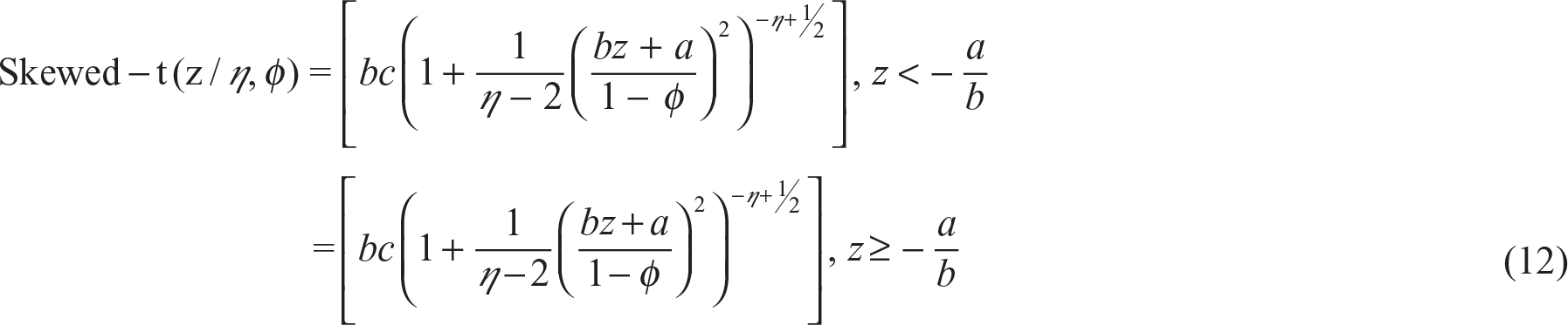
The values of a, b and c are defined as:

where η is the parameter for kurtosis (kurtosis being measure of the peakedness as well as fat tailedness of the distribution) and ϕ is the asymmetric parameter. The restrictions for η and ϕ are: 2 < η < ∞ and −1 < ϕ < 1. When ϕ = 0, then the normal distribution is obtained, while the Student-t distribution for ϕ = 0 and for η → ∞ Like the Student-t distribution, it is well defined only for η > 2, the skewness exists only for η > 3, and the kurtosis exists only if η > 4. The mode of density is to the left of 0 and the variable is skewed to the right, in case ϕ > 0; vice- versa for ϕ < 0.
Patton (2006) has suggested that the Kolmogorov–Smirnov (K–S) test should be performed to test the empirical adequacy of the marginal models. This test has been suggested as modelling copulas would require a model for marginal distributions to be distinguishable from the true ones. The probability integral transforms will be non-uniform (0, 1) if a misspecified model is used for the marginal distributions. If a misspecified model is used, any copula model will automatically be misspecified.
A Gaussian copula and a Student-t copula are usually the best choice of an elliptical copula, which is used for the dependence structure. They are defined by:


When the weight of the joint density in one or both tails is larger than that of a multivariate normal density, it is referred as a tail dependency. In a multivariate setup, the fat tail phenomenon is known as a tail dependency. Suppose an event in X occurs whose probability is less than v. Also, an event has occurred with probability lower than Y, the formula for tail dependence will be as follows:


where C ( , ) is the CDF of the copula and F
X
( ) and F
Y
( ) are the marginal CDFs for X and Y, respectively. Symmetric tail dependencies are presented by Gaussian and Student-t copulas which are given by
The SJC copula considers the lower and the upper tail dependence, whereas the Clayton copula considers only the lower tail dependence. The SJC copula’s dependence measures completely determining the presence or absence of symmetry.
The formula is as follows:
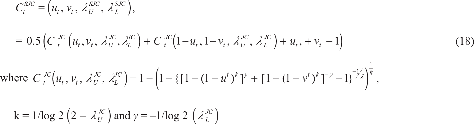
Also,
In this article, we have considered Kendall’s τ as the main measure of association, since contagion is considered to be a non-linear phenomenon (Rodriguez, 2007). The linear correlations cannot capture the non-linear dependencies 1
The non-linear dependence parameters have been captured based on Equations (19)–(21) as given in the Methodology section.
The copula function allows modelling the dependency between series (both linear and non-linear) which do not follow the same distributions, inclusive of non-normal distributions. However, when using non-linear methods like M-GARCH, the estimation becomes highly complex if we deviate from the assumptions underlying the multivariate models. Moreover, estimating the time-varying non-linear dependence parameters using copula approach requires much less computational resources and estimation time in comparison to the computational resources and estimation time required in the multivariate GARCH family models. That’s why, now, the risk management industry is more inclined towards using copula for estimating dependence parameters to quantify both market and credit risks.

Equations (19) and (20), respectively, define the evolution of upper and lower Kendall’s τ for the SJC copula (Patton, 2006).


Data and Analysis
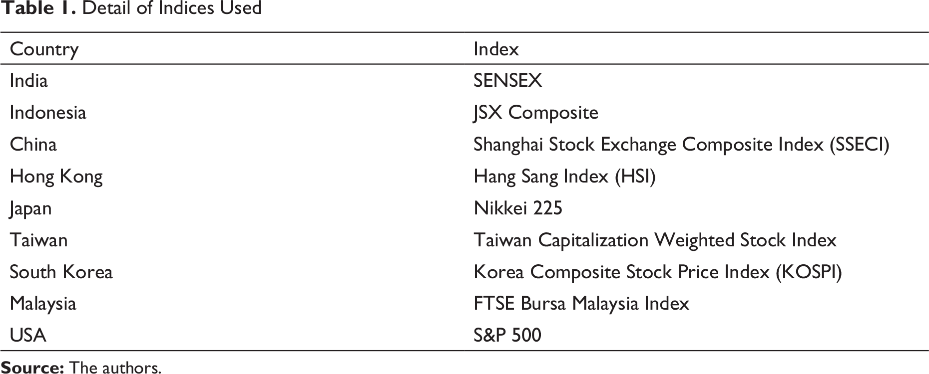
Data employed in this study are log returns 2
Log returns = Log [P t /(Pt−1)].
The period of 8 years from January 2004 to December 2011 (1,486 observations for each country) has been studied. The data have been compiled from BLOOMBERG.
Detail of Indices Used
Descriptive Statistics
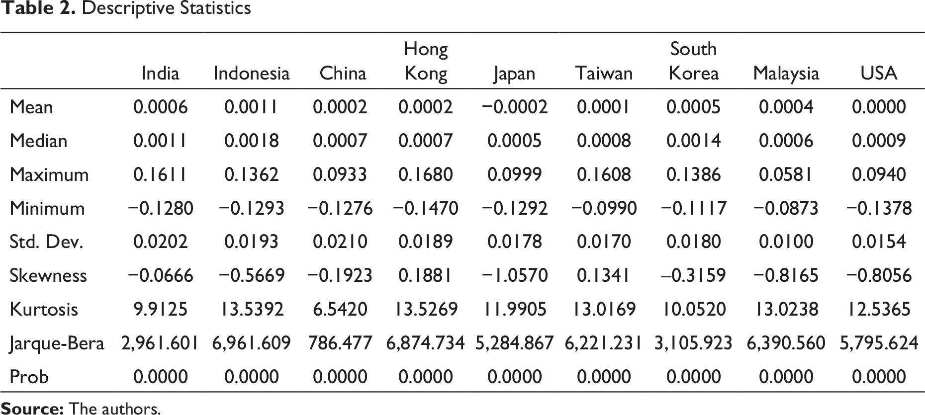
Table 2 describes the data and shows that out of all Asian markets under study, only Japan has negative mean returns over the period of the study; whereas Indonesia has the highest mean returns. While measuring standard deviation, it was found that Malaysia has the lowest standard deviation in returns while China has the highest. Taiwan and Hong Kong show positive skewness while all other stock markets show negative skewness in the return series. Kurtosis for all markets was above 3 which means that all the countries’ series are Leptokurtic.
Maximum Likelihood Estimates of Copula
Maximum Likelihood Parameter Estimates of Gaussian and SJC Copula for the US and Asian Economy Pair
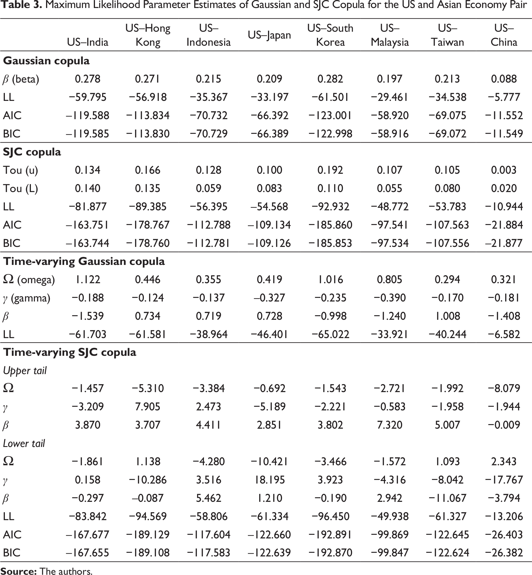
Results based on the Gaussian copula for US–China pair shows that the correlation coefficient is close to zero, implying low level of persistence in correlation between the US market and the Chinese market which indicate that any shock to one market can drift the correlation between markets, away from the long-run equilibrium value/position for a very short period. Following Hsu, Tseng, and Wang (2008), if the coefficient value is close to 1, the correlation between the two stock markets is considered to be highly persistent. High persistence in correlation would mean that if a crisis hits a market, then the correlations between the markets will get pushed away from its long-run average for a significant period. While correlations have a tendency of reverting to its mean position, a low persistence level would lead to slow movement of correlations away from long-run equilibrium level. If the series demonstrates non-linear behaviour in the joint and marginal distributions of assets, it may show a high level of persistence in correlations (De Lima, 1998). For all the other pairs of markets except US–China, the correlation coefficient estimates of the Gaussian copula lie between 0.2 and 0.3 which is relatively higher than what we observed for the US–China pair. The persistence level indicates that any shock to US stock markets will push the correlation between markets away from the long-run average value for a shorter period but not as short as the case with the US–China pair. Results based on SJC copula support the presence of significant lower and upper tail dependence for all the pairs except for US–China pair. We have compared the log-likelihood values, AIC and BIC of Gaussian copula and SJC copula for all pairs to examine which model better captures the dependence dynamics between the market pairs. The three measures (Log-likelihood, AIC and BIC) suggest that SJC copula better captures the dependence dynamics of the market pairs than the normal copula for all the pairs of stock markets under study. Moreover, the SJC copula can capture the lower as well as upper tail dependencies between the market pairs which is not the case with the Gaussian copula.
It is to be noted that the dependence structure between markets changes over time and are more likely to be influenced by various macroeconomic events. Hence, a constant correlation model or a constant dependence copula model would not be appropriate for defining dependence between markets. Thus, we also estimate the time-varying Gaussian and SJC copula to highlight the variations in the dynamics of dependence structure of the various market pairs. The β (beta) coefficient of the time-varying SJC copula indicates that if there is an upward variation in levels of the index value of one economy, then what would be the effect on the level of the index of another economy in the pair. The upper tail dependence parameter of the time-varying SJC copula is positive for all the market pairs with the exception of the US–China pair, for which it is negative. Positive upper tail values suggest that if the stock prices would increase in US market, then correspondingly they would increase in other Asian markets for which upper tail values are positive. If the upper tail values of SJC copula are negative, as in the case of US–China pair, it would suggest that a decrease in stock price in US market would lead to decrease in stock prices in Chinese stock market. The values of Log-likelihood, AIC and BIC indicate that the time-varying SJC copula comparatively better captures the time-varying dependence in all the market pairs under study.
On observing the time-varying Gaussian copula coefficients, following things were examined. The degree of persistence is measured by β, whereas γ (Gamma) represents the adjustment that is made in the dependence process. The negative values of γ indicate significant variations over time for all the pairs of stock markets. The larger variation in the dependence structure has been observed for two pairs, that is, US–Japan and US–Malaysia as modulus values of γ is higher for these two pairs in comparison to other pairs.
If we look at the results for normal copula of the USA and India (Figure 1), we can see that the time-varying dependence structure changes significantly during the period of sub-prime crisis (as evidenced by the sudden change in time-varying correlation graph between observations 500 and 1,000). During the pre-crisis period (time-varying correlation graph between observations 0 and 500), the dependence structure is less volatile, and this is also observable during the post-crisis period (time-varying correlation graph between observations 1,000 and 1,500). We can infer similar findings from the plots for all the other pairs under study. For all the given pairs, we can see that the dependence structure between the US stock market and the respective market took a sharp plunge between the observations 500 and 1,000. By carefully looking at a time-varying correlation based on the normal copula for the pair US–Hong Kong pair, one can infer that during the pre-crisis period, the dependence structure was not very volatile and similar characteristics are also observed during post-crisis period. During the crisis period, the time-varying dependence structure exhibits significant decline, showing how the Hong Kong stock market reacted to the US housing bubble of 2007–2008. Similar findings can be inferred for US–Japan pair and US–South Korea pair. The US–Taiwan pair depicts very high volatility in the time-varying dependence structure during the crisis period which continues during the post-crisis period too. For US–Malaysia pair, the time-varying dependence structure during the crisis period and post-crisis period are highly volatile, whereas for US–Indonesia pair, high volatility in the dependence structure can be seen only during the crisis period. For the US–China pair, the fall in the dependence structure might not look so drastic as in other cases. This, however, does not mean that the Chinese markets were not affected during the 2008 crisis period. While interpreting the results, one needs to see that there is a change in the time-varying dependence structure over time. The sudden change in the dependence structure can be related to the evidence of the existence of contagion which is common across most of the pairs during the sub-prime crisis period. This is further validated by the results of Figure 2.
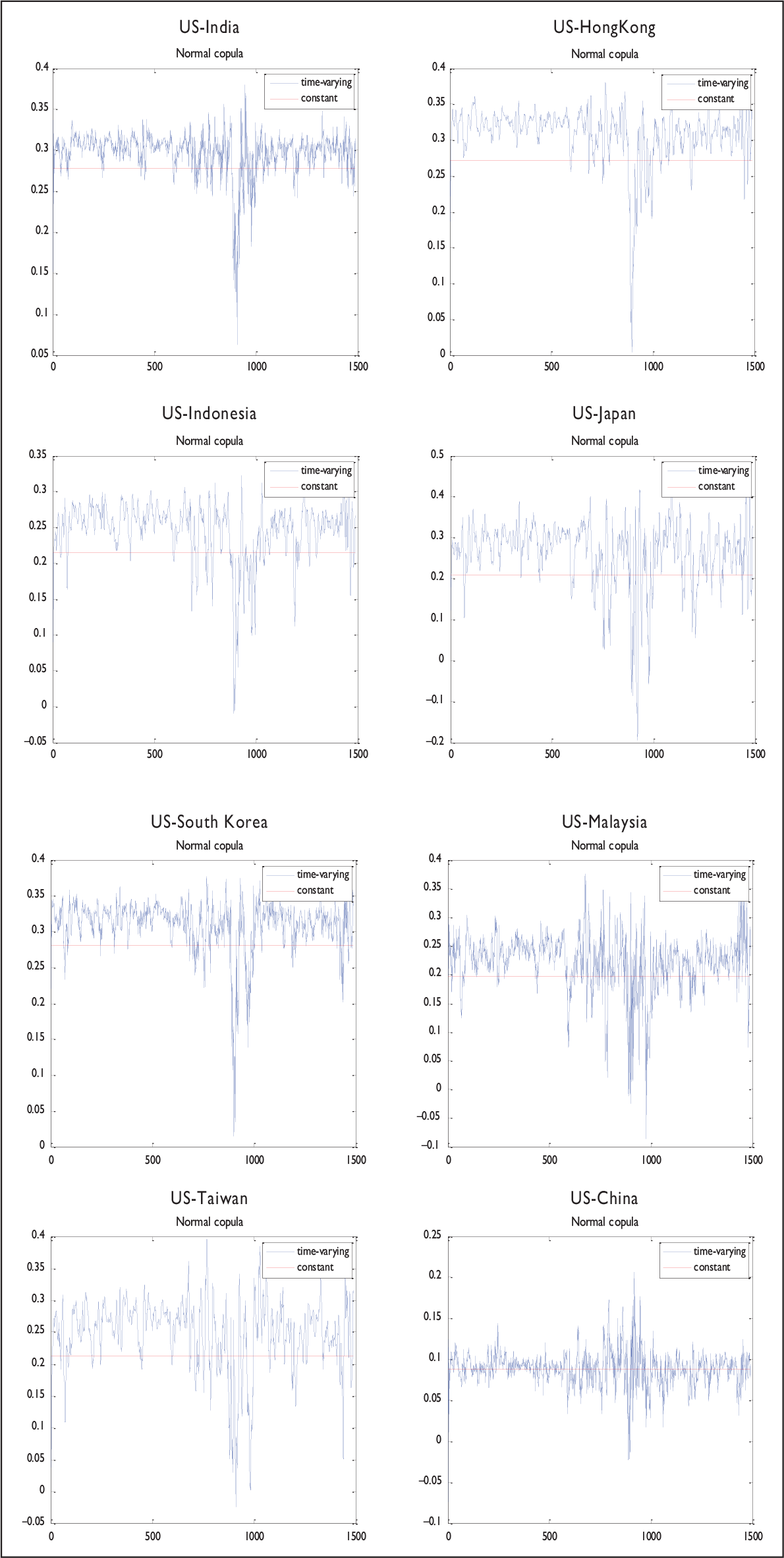
The numbers on the X-axis represents the dates, where 1 represents ‘01-01-2004’ and 1,500 represents ‘19-12-2011’. The number is used by the software as the plots are the output of the analysis.
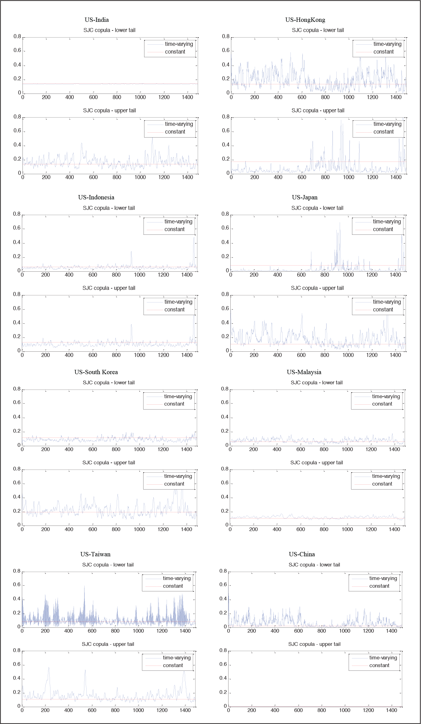
The numbers on the X-axis represents the dates, where 1 represents ‘01-01-2004’ and 1,500 represents ‘19-12-2011’. The number is used by the software as the plots are the output of the analysis. Y-axis represents constant and time-varying SJC copula.
When a market crashes or during periods of high volatility, the financial returns of that country do get impacted. To assess the joint extreme events during such periods of turmoil, tail dependencies prove to be useful. Figure 2 demonstrates lower and upper tail dependencies based on the SJC copulas for all the pairs under study; the blue line depicts the time-varying dependence structure, whereas the red line shows the dependence structure based on the whole sample between the two markets of the pairs under study. The literature suggests that in the case of equity returns, joint-negative extremes are reflected more than joint-positive extremes. This leads one to assume that upper tail dependencies are less strong than lower tail dependencies. From Table 3, we can see that Ω L SJC (Omega of SJC copula of lower tail dependence) is higher than Ω U SJC (Omega of SJC copula of upper tail dependence) for most of the cases. This further implies that the lower tail dependence is higher than upper tail dependence.
After observing the lower tail dependence of the US–India pair based on the SJC copula, it can be said that the lower tail dependence between the USA and India does not vary much which is depicted by the blue line in the graph. The red line in the graph shows that the dependence structure between the USA and India is quite near to 0.2 which further does not vary over time. However, the upper tail dependence exhibits dynamic behaviour and varies a lot. The table values of Kendall Tau showing average dependence (upper and lower) are shown as Tou (u) and Tou (L) in Table 3 under SJC copula. It can also be seen that during the period of sub-prime crisis, the upper tail dependence between the USA and India exhibit wider variation which indicates that the upper tail dependence between India and the USA is much stronger than the lower tail dependence. These results indicate that the extent of the impact of downfall during the period of sub-prime crisis was not that much for India as it was for other economies under study.
On the other hand, for the US–China pair, the lower tail dependence is much stronger than the upper tail dependence as depicted by the US–China SJC copula plot. The upper tail plot shows that the time-varying dependence structure does not vary much. This indicates that when the market is trending down, the risk management and diversification strategies becomes less effective if there is stronger lower tail dependence. Hence, the focus of risk managers should be on the lower tail during such periods while designing portfolio rebalancing and risk management strategies. This can help the risk managers and regulators to avoid the condition of the joint crash.
The tail dependence coefficients in empirical findings are based on the Equations (16) and (17) as given in Methodology section and are estimated using Maximum Likelihood estimation. Tail dependence measures association between the extreme values of two random variables and depends only on their copula. If there are no tail dependencies among the returns of the series in a portfolio, then there is little risk of simultaneous very negative/positive returns, and the probability of occurrence of an extreme negative/positive return on the portfolio is low. However, if there exist tail dependencies, then the probability of occurrence of extreme negative/positive returns simultaneously can be high. Hence, it is important to consider tail dependence when assessing the diversification benefit and risk of any portfolio.
The impact of the global financial crisis has led to sudden changes in the dependence structure between the USA and Indonesia stock markets. The results related to lower tail dependence shows that there has been higher volatility in dependence parameter throughout the period, whereas the results for upper tail dependence shows that there has been very less or rather negligible volatility in the dependence structure during the period under study.
There is a sudden change in dependence structure between the USA and Japan stock markets due to the impact of the global financial crisis. The lower tail parameter remains constant during the pre-crisis period. During the crisis period, the dependence structure reacts towards the US sub-prime crisis. For US–Indonesia pair, one can observe that the time-varying dependence structure does not vary much. It is nearing the constant red line depicted in the plot. This shows that there is not much volatility in the dependence structure between US–Indonesia pair. Similar results can be inferred for US–Malaysia pair. The US–Taiwan’s SJC copula lower tail shows too much of volatility in the time-varying dependence structure between the two countries’ stock market prices which shows that the Taiwan stock market did get impacted due to the financial crisis of 2007–2008 which started in the USA. For US–South Korea pair, the lower tail dependence structure is less volatile than the upper tail.
Our findings support the presence of sudden changes in dependence structure for the given pairs under study. We also observe an increase in conditional tail dependence (lower) for US–Hong Kong, US–Indonesia, US–Japan, US–Taiwan and US–China pairs. The increase in conditional dependence structure can be related to the presence of evidence of contagion. We also observe an increase in upper tail dependence over a period for US–India, US–Hong Kong, US–Indonesia, US–Japan, US–South Korea and US–Taiwan pairs. This increase in tail dependence in the given market pairs can also be related to evidence of contagion. If there are no tail dependencies among the returns of the series in a portfolio, then there is little risk of simultaneous very negative/positive returns, and the probability of occurrence of an extreme negative/positive return on the portfolio is low. However, if there exist tail dependencies, then the probability of occurrence of extreme negative/positive returns simultaneously can be high. Hence, it is important to consider tail dependence when assessing the diversification benefit and risk of any portfolio.
Conclusion
The copula methodology has enabled us to examine contagion from US stock market to few selected Asian stock markets including India. As discussed earlier, the advantage of copula over other methodologies is that it examines the non-linear dependence among markets. The copula methodology has pointed out that the Asian stock markets have experienced contagion effect due to a sub-prime crisis whose epicentre is the USA. The copula methodology also focuses on the tail dependence structure of the series. The results indicate that for few countries, the impact of the global financial crisis has led to sudden changes in the dependence structure between the US and the respective stock markets. For others, like the US–China pair, the lower tail dependence is much stronger than the upper tail dependence, indicating that the government might have come up with a lot of policy measures to be able to withstand any crisis that would occur in future. However, lower tail dependence being stronger than upper tail shows that in the event of trending down market, the risk and diversification strategies become less effective, that is, the policy measures that the government had taken before such crisis did not prove to be effective during tranquil times. The other extreme case is that of India–US pair where upper tail dependence is much stronger than the lower tail dependence which shows that the Indian stock markets reacted quite late to the housing bubble that took place in the USA in 2007–2008. Thus, the results clearly show that the Asian markets were influenced significantly by the US sub-prime crisis.
The findings of the present study suggest that Asian economies might have got affected due to the ripple effect of the crisis. This means that when US financial markets were facing liquidity crunch, the Foreign Institutional Investors (FIIs) pulled out the money invested in other parts of the world in order to fulfill the liquidity requirements in the USA. The bulk selling of shares in Asian markets by FIIs led to panic situation and many uninformed investors would have also sold their holdings without much understanding the situation. This led to falling in share prices, and continuous fall would lead to depressive sentiments of investors, thus further deteriorating the condition in the stock market.
The copula approach helps us to generate estimates of the time-varying correlation measures. This can help the practitioners to compute hedge ratio and has important implications towards portfolio management and risk management. Moreover, the time-varying estimates of correlations and tail dependence can help to better understand the co-movement relationship in the asset classes and also can help the traders to develop profitable trading strategies. Not only this, the time-varying estimates of correlations and tail dependence can help the policymakers to better understand the dynamic relationship between the markets and the impact of any macroeconomic shock from one market to the other and can develop policies to reduce the impact of the possible shock originated in another market to self-market.
Footnotes
Acknowledgement
The authors are grateful to the anonymous referees of the journal for their extremely useful suggestions to improve the quality of the article. Usual disclaimers apply.
Declaration of Conflicting Interests
The authors declared no potential conflicts of interest with respect to the research, authorship and/or publication of this article.
Funding
The authors received no financial support for the research, authorship and/or publication of this article.