Examining the Role of Policy and Cultural Determinants on Sectoral Export Competitiveness: Evidences from India

Abstract

Exports are affected by several economic, political, social and cultural determinants. The objective of this study is to examine the role of policy and cultural determinants on export competitiveness for different sectors, estimate the technical efficiency (TE) and suggest focus areas to improve exports. The study uses the method of stochastic frontier analysis on the bilateral trade of India over the period 2000–2016. The result findings highlight that there is underutilization and ambiguous effect of trade agreements for all sectors except intermediate goods (IGs). Foreign direct investments outflow has positive results for all the sectors with capital goods getting benefitted the most. TE of exports shows positive trends for IGs, negative trend for raw materials, and mixed trend for consumer goods and capital goods sectors. IGs show the best export competitiveness, whereas RMs have the highest export potential. The results underline India’s progress in integrating with the global supply chain through increasing TE in exports of IGs.

Keywords

Export competitiveness policy culture stochastic frontier analysis trade efficiency

Introduction

The buoyant world economy and competitiveness are key determinants of exports (Rangarajan & Kannan, 2017). There is substantive literature on the role of economic, political, social and cultural determinants on exports competitiveness (Brodzicki & Uminski, 2013; Felbermayr & Toubal, 2010; Gokmen, 2017; Guzman, Ocampo, & Stiglitz, 2018). Several studies (Atif, Haiyun, & Mahmood, 2017; Seleka & Kebakile, 2017) have focused on the export competitiveness in specific industries like beef industry or sectors like agriculture. Few studies (e.g., Bhagavan, 1985; Francis, 2011) have explored some aspects of exports competitiveness products based on classifications on levels of processing and stages in the value chain.

In the 1950s, like many other developing economies, India adopted import substitution policies to encourage the domestic industrial sector. The policy of retaining restrictions and high tariff rates for such a long period resulted in low growth rate, overvalued exchange rate and inefficient industries (Jain, 2017). India’s share in world merchandise exports was 1.39 per cent during 1950–1959, which came down to 0.48 per cent during 1986–1990 (Veeramani, 2007). However, in the post-economic reform period, India’s export growth rate was not distinctly high until 2000 (Veeramani, 2007). Table 1 shows India’s exports for 2000–2016 with all its trading partners. India’s exports experienced a continual decline since 2013. India is facing high trade deficits in consumer goods (CoG) and intermediate goods (IG), which belong to labour-intensive industries due to cheaper labour and low trade costs in other countries like Vietnam and China, and agricultural products are facing stringent non-tariff barriers and unproductive trade agreements. There are negative effects of domestic demand pressure, and low investment and limited technological capabilities are reducing the export competitiveness (Mohanty & Sethi, 2019).

Table 1.

Trade Statistics

Year	GDP (current)*	Exports*	Exported Products	Export Partners
2000	462.14	42.36	4,501	212
2001	478.97	43.88	4,577	212
2002	508.07	50.1	4,649	213
2003	599.6	59.36	4,662	217
2004	699.69	75.904	4,695	222
2005	808.9	100.35	4,696	223
2006	920.32	121.2	4,692	221
2007	1,201.11	145.9	4,664	221
2008	1,186.95	181.86	4,691	222
2009	1,323.94	176.76	4,467	222
2010	1,656.62	220.41	4,462	223
2011	1,823.05	301.48	4,483	220
2012	1,827.64	289.57	4,460	221
2013	1,856.72	336.61	4,444	221
2014	2,035.39	317.55	4,434	221
2015	2,111.75	264.38	4,424	220
2016	2,263.52	260.33	4,411	219

Source: UN Comtrade.

Note: *In USD billion.

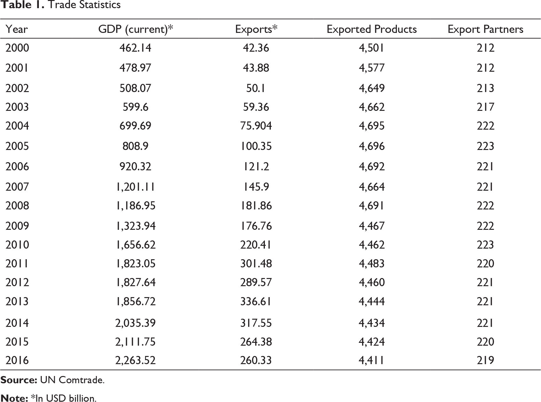
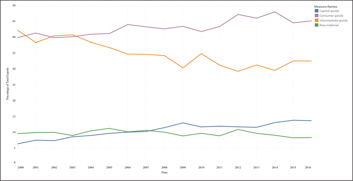
The export competitiveness at different stages of the production process provides varying influence and capabilities in the value chain. However, there is scant literature on the inter-sector wise analysis of export competitiveness and varying effects of key determinants on the export performance. This study makes the distinction by comparing the effects of different factors determining the export competitiveness based on the level of processing and stages in the value chain. This kind of comparative study puts forth the differences in country-level factors affecting the four sectors, which were overlooked in previous studies. This study refers to four product groups (RM, IG, CoG and CaG) at different stages of production as the different sectors for analysis. In contrast, most studies focussed on either export as a whole or studied a specific industry or product category such as agricultural sector or textile industry. Our study fills this gap by applying stochastic frontier analysis (SFA) on India’s export competitiveness for different sectors. The use of production function in SFA gives the maximum possible extent of exports that can take place to a particular country.

The remaining of the article is as follows: the second section reviews the literature, the third section outlines the objectives and rationale of the studies, the fourth section discusses the methodology adopted, the fifth section portrays the analysis, the sixth section discusses the results and the seventh section draws conclusions and implications.

Review of Literature

The article reviews the literature from two perspectives. First, the literature is reviewed on the cultural, policy variables and other country-specific control variables affecting the exports. Second, literature review is carried out on the studies employing gravity model estimation and stochastic frontier approach. Ghemawat (2001) highlighted the significance of cultural, administrative, geographic and economic factors on exports. Indian exports growth indicators neither remain consistent nor remain homogenous across export basket for several such reasons (Doan & Xing, 2018; McDonald, Robinson, & Thierfelder, 2008). McDonald et al. (2008) discussed India’s non-integration into cross-country production chains and examined the impact of economic structures and trade patterns on exports. The determinants of cultural proximity also act as the proxy for the cost of communication, which affects export competitiveness (Felbermayr & Toubal, 2010). Carrere (2006) found that an increase in the number of trade agreements increases exports, due to reasons such as the decrease in tariffs, non-tariff barriers and improvement in export competitiveness (Doan & Xing, 2018). Financial flows influence the export competitiveness of an economy (Brodzicki & Uminski, 2013). FDI has several objectives, such as seeking resource, efficiency, market or strategic assets. Mohanty and Sethi (2019) associated FDI with increased trade, technology transfer, employment and integration in the global supply chain while Athukorala (2009) argued that FDI outflow contributes to improving the export competitiveness and opening of new market opportunities. Thus, FDI incorporates factors related to technology, market and knowledge transfer, which ultimately contributes to improved firm efficiency and productivity. McCallum (1995) identified the ‘border puzzle’ for the interprovincial and province-state trade of the United States and Canada. Frankel, Stein, and Wei (1995) argued that regional trading blocs along with time-invariant dummies like common language and common borders contribute to the increase in trade flow. Head, Mayer, and Ries (2010) investigated the decreasing but existing effect of colonial links. Other control variables that affect the exports are GDP, which behaves as a proxy for the expenditure and the production functions. Isard and Peck (1954) first explained the negative relationship of distance with domestic as well as international transport. Trade costs linked with tariffs, regulations and exchange rates vary inversely with the elasticity of demand in sectoral classification (Doan & Xing, 2018; McDonald et al., 2008). Bergstrand (1985) found empirical evidence of exchange rates significantly affecting the export competitiveness. Exchange rate movements affect trade by creating uncertainty about future costs in global transactions (Eregha, 2019). Martínez-Zarzoso and Nowak-Lehmann (2003) found that the population of the partner countries have a significant and positive association with the exports level of the exporting country. Ravishankar and Stack (2014) found high technical efficiency (TE) between countries lying in eastern and western part of European Union, while Atif et al. (2017) found low TE for Pakistan’s agricultural products with its neighbour India.

One of the earliest studies examining the determinants of exports using gravity model of trade was done by Tinbergen (1962). Anderson (1979) derived the same equation through constant elasticity of substitution (CES) preferences, Helpman and Krugman (2002) through product differentiation model, Bergstrand (1985, 1989) by establishing the relationship between trade theory and bilateral trade and Deardorff (2011) through the new trade theory. However, empirical gravity model overlooked the overall average barriers that countries engaged in bilateral trade face from their other trading partners. Anderson and Wincoop (2003) analyzed importer and exporter specific factors, access to the market for the exporter and exogenous factors like nature of the market economy and trade liberalization as the key determinants of export. Anderson and Wincoop (2003) suggested country-specific price-raising effects to measure multilateral resistances. Baier and Bergstrand (2009) established the theoretical relationship between bilateral and multilateral resistances and recommended simple averages instead of GDP-share weight for calculating multilateral resistance.

SFA is used to estimate the maximum values of any production function, exports in this case, and to further assess the possible expansion (Mahadevan & Gonemaituba, 2013). Aigner, Lovell, and Schmidt (1977) first formulated SFA to estimate the industry production function using a linear model for cross-section data by defining the error specifications. SFA model contains two error terms given in equation (1), u_ij is the economic distance bias error term and v_ij is the error term, which captures the effect of all the factors not accommodated in the estimation model (Kalirajan, 2007). SFA approach investigates the regulatory, economic, and policy reforms (Armstrong, Drysdale, & Kalirajan, 2008). OLS estimation is used to check the robustness of the SFA approach (Bauer, Berger, Ferrier, & Humphrey, 1998). One of the significant differences between these two methods of analysis is in the treatment of its error term.

Objectives and Rationale of the Study

The main objective of the study is to examine the role of policy and culture variables on the export competitiveness of different product classification based on stages of processing and stages in the value chain. To the best of our knowledge, studies have not shed light upon such aspects, conditions and factors due to which exports of a country varies across different levels of processing and stages in the value chain. Another objective of the study is to find the impact of cultural and policy variables on the TE with major trading partners of India. Export competitiveness of products based on classifications on levels of processing and stages in the value chain is determined by both, country-level factors as well as firm-level factors. For example, determinants of agricultural goods are largely country-specific factors such as food safety and standards, low trade costs and export orientation whereas determinants of manufacturing goods are related to an extent to firm-specific factors such as technological know-how. However, Filippini and Molini (2003) in their analysis of exports of manufactured goods and non-manufactured goods used country-specific variables. Since the main objective of the study is to examine the effects of culture and policy variables, this study is focusing upon country-specific factors.

Methodology

Data Source and Sample

The panel data set for our analysis consists of India’s bilateral trade flows with its partners over 2000–2016. The sectors are classified under the Harmonized System (HS) 1988/92 product nomenclature. The data for bilateral exports are obtained from UN Comtrade database through WITS software. Table 2 depicts all the independent variables, their definitions and data sources. The data for GDP are obtained at constant year 2010 USD. The effect of simultaneity is taken care of by taking export in a lagged form (Pradhan, 2004). All the continuous variables are taken in a natural log form for the analysis. Figure 1 shows the changing composition of India’s exports over 2000–2016. CoG have been sharing the maximum share in the export basket since 2003. CaG remains steady at around 10 per cent, and there is a decline in raw materials (RMs) since 2012.

Table 2.

Variable Description and Data Source

Variable	Description	References	Data Source
FDI	Measure of financial flow to gauge export orientation and technical know-how	Athukorala (2009), Brodzicki and Uminski (2013)	WDI
TA	Measure of trade barriers. Increase in trade agreements reduces the trade barriers	Doan and Xing (2018), Carrere (2006)	CEPII
Contig	Common border lead to easier transportation. Expected to cause increase in trade flows	McCallum (1995), Mishra, Gadhia, Kubendran, and Sahoo (2015)	CEPII
comcol	Colonial linkage lead to administrative similarities. Expected to cause increase in trade flows	Head et al. (2010), Atif et al. (2017)	CEPII
comlang	Common language lead to easier transactions. Expected to cause increase in trade flows and reduction in transaction cost	Frankel et al. (1995), Head et al. (2010)	CEPII
GDPi	Production function of the exporter. Measure of ability to export. A high level of income in the exporting country indicates a high level of production, which increases the availability of goods for exports	Tinbergen (1962), Ravishankar and Stack (2014)	WDI
GDPj	Expenditure function of the partner. Measure of ability to import. A high level of income in the importing country indicates a high level of consumption, which increases the possibility for import of goods	Tinbergen (1962), Ravishankar and Stack (2014)	WDI
Distance	Measure of trade/transport cost	Isard and Peck (1954), Anderson and Wincoop (2003)	CEPII
Population	Expenditure function of the partner. Measure of ability to consume. Population has a large and positive effect on exports, indicating that bigger countries import more than small countries	Martínez-Zarzoso and Nowak-Lehmann (2003), Filippini and Molini (2003)	WDI
ex-rate	Affects returns on investments. Exchange rate depreciation can make the investments more profitable	Bergstrand (1985), Atif et al. (2017)	WDI

Source: The authors.

Figure 1.

Source: WITS.

Empirical Model

The model specification for our analysis consists of two methods. The first method of analysis is the SFA approach, and its equation is the log-linearized form of modified gravity model. Sanso, Cuairan, and Sanz (1993) found that the log-linear transformation is a fair approximation of an optimal form. Additionally, several studies have applied the gravity model using the log-linearized form (Atif et al., 2017; Mishra et al., 2015; Ravishankar & Stack, 2014).

\begin{array}{l} B i l a t e r a l T r a d e = β_{0} + β_{1} F D I_{i t} + β_{2} T A_{i j t} + β_{3} c o n t i g_{i j} + β_{4} c o m c o l + \\ β_{5} c o m l a n g_{i j} + β_{6} G D P_{i t} + β_{7} G D P_{j t} + β_{8} d i s \tan c e_{i j} + β_{9} p o p_{j t} + β_{10} e x_r a t e i_{j t} - u_{i j} + v_{i j} \end{array}

(1)

where

FDI_it is the FDI outflow from the exporter country,

TA_ijt is the dummy variable for the status of preferential trade agreements,

contig_ij is the dummy variable for the common border between trading countries,

comcol_ij is the dummy variable for common colonial links,

comlang_ij is the dummy variable for common language,

GDP_it and GDP_it are the GDP of the exporter and partner countries,

distance_ij is the geographical distance between the most populous cities of the two countries,

Pop_jt is the population of the partner countries,

ex_rate_ijt is the bilateral exchange rate;

the subscript t denotes the time-varying nature of the variable and explains the values for given year t. u_ij and v_ij are the error terms. The results also generate additional parameters given as

λ = \frac{σ (u_{i})}{σ (v_{i})}

(2)

σ^{2} = σ_{v}^{2} + σ_{u}^{2}

(3)

γ = \frac{σ_{u}^{2}}{σ^{2}}

(4)

The value of γ explains the good fit of the estimation model, σ² is the composed error term and λ explains the degree of inefficiency relative to the random error (Ravishankar & Stack, 2014). The estimation efficiency of this model does not suffer any loss because of the isolation of the single-sided error term for technical inefficiency, u_i The comparative analysis of the observations of this specification model is done with the respective observations obtained from the OLS estimation.

However, Equation (1) consists of a trade cost function, which does not take the systematic bias and the exogenous factors into account such as changes in any bilateral route will incorporate trade diversion or creation for other trade routes. The variables of trade cost are given in Equation (5). The equation is further treated for multilateral resistances as given in Equation (6), where

τ_{i j} = f (d i s t a n c e_{i j}, t r a d e a g r e e m e n t s_{i j t}, c o m c o l_{i j}, c o n t i g_{i j}, c o m l a n g_{i j})

(5)

\ln τ_{i j}^{*} = \ln τ_{i j} - \sum_{j = 1}^{M} θ_{j} \ln τ_{i j} - \sum_{i = 1}^{N} θ_{i} \ln τ_{i j} + \sum_{j = 1}^{M} \sum_{i = 1}^{N} θ_{i} θ_{j} \ln τ_{i j}

(6)

and,

θ_{i} = G D P_{j} / G D P_{w o r l d}

(7)

This estimation model brings endogeneity bias in the adjusted variable (Baier & Bergstrand, 2009). The biasness is removed by replacing the GDP -weighted share with the simple averages between distance clusters. Under the assumption of symmetric bilateral trade costs, the simple average method gives identical second and third term as

\frac{1}{N} \sum_{i = 1}^{N} \ln τ_{i j} = \frac{1}{M} \sum_{j = 1}^{M} \ln τ_{j i}

(8)

Therefore, the specification model for multilateral resistances adjustment is written as

\ln τ_{i j}^{*} = \ln τ_{i j} - \frac{1}{N} \sum_{j = 1}^{N} \ln τ_{i j} + \frac{1}{2} \frac{1}{N^{2}} \sum_{j = 1}^{N} \sum_{i = 1}^{N} \ln τ_{i j}_{}

(9)

where N is the number of distance clusters.

In the second part of the analysis, the TE for exports is estimated (Atif et al., 2017; Battese & Coelli, 1995). The range for TE is 0 to 1 where one denotes that actual export has coincided with export potential while any number between 0 and 1 denotes the gap between actual export and export potential for the given country-pair. The calculations for TE of exports are carried out for its major trading partners, including all the neighbourhood countries, which have geopolitical and cultural significance. The results are divided for two subperiods and the average TE is calculated for all the sectors. The TEs of the two subperiods are then used to calculate the TE ratio (TER) as

T E R = \frac{T E 2}{T E 1}

(10)

TE1 and TE2 are the TE for the time period 2000–2008 and 2009–2016, respectively. For TER greater than 1, it shows that TE has improved, otherwise deteriorated, where 1 being the neutral point. For the sake of comparison, the neutral point is adjusted to zero using the following equation:

A T E R = (\frac{T E 2}{T E 1}) - 1

(11)

Analysis

The summary statistics of all the variables of our model specification is shown in Table 3. There is a broad range of export (6.09, 24.35) with 17.86 mean and 2.70 standard deviation. The range of importer GDP (17.21, 30.36) explains the heterogeneity in the partner countries. The mean values for contiguity and trade agreements highlight the high degree of interregional exports and multilateralism.

Table 3.

Summary Statistics

Variables	Mean	Std. Dev.	Minimum	Maximum	Observations
Exports	17.86	2.7	6.09	24.35	2,663
Exporter GDP	27.95	0.35	27.41	28.53	2,663
Importer GDP	23.86	2.31	17.21	30.46	2,663
Importer population	15.52	2.07	9.48	21.04	2,663
Distance	8.76	0.67	6.53	9.74	2,663
Exchange rate	–0.66	2.76	–6.92	18.86	2,663
FDI outflow	22.34	1.18	20.05	23.68	2,663
Contiguity	0.04	0.19	0	1	2,663
Colony	0.35	0.48	0	1	2,663
Common language	0.32	0.47	0	1	2,663
Trade agreements	0.8	0.4	0	1	2,663

Source: The authors.

Note: Std. Dev. = Standard deviation.

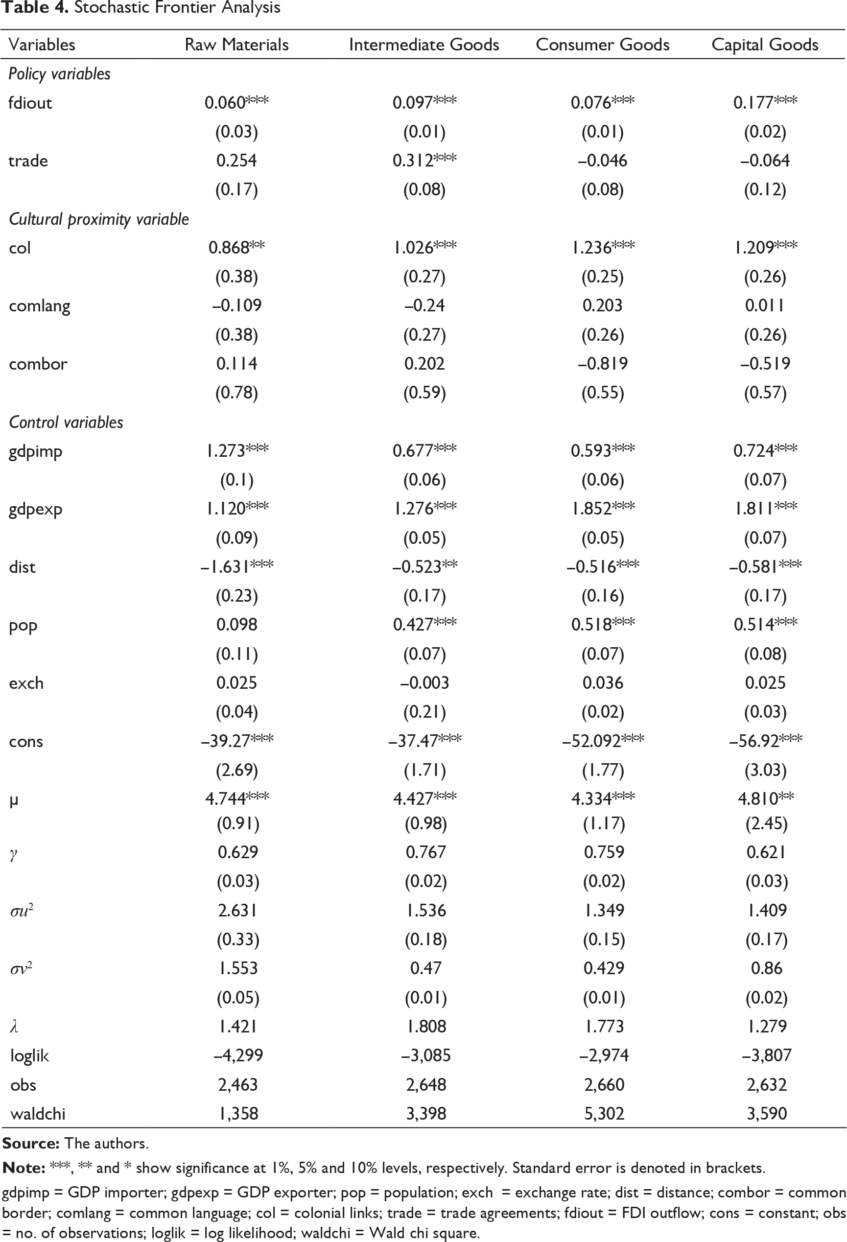
SFA approach for all the classification gives statistical significance with expected signs. The values for λ being greater than 1 explains the degree of inefficiency in the estimation models. The statistical significance of µ justifies the SFA approach. The values for γ are between 0 and 1, explaining the influence of country-specific constraints such as institutional and sociopolitical factors. The values for γ are closer to 1, which highlights that the estimation models are a good fit (Battese & Coelli, 1995).

The results of the estimation model pertaining to SFA are given in Table 4. The empirical results for the sector-wise analysis is as discussed, RM have importer GDP (1.273), distance (–1.631) and colonial links (0.868) as the key determinants; IG have exporter GDP (1.276), importer GDP (0.677), importer population (0.427) and trade agreements (0.312) as the key determinants, CoG have exporter GDP (1.852), colonial links (1.236) and importer GDP (0.593) as the key determinants, and CaG have exporter GDP (1.811), colonial links (1.209) and FDI outflow (0.177) as the key determinants of export competitiveness.

Table 4.

Stochastic Frontier Analysis

Variables	Raw Materials	Intermediate Goods	Consumer Goods	Capital Goods
Policy variables
fdiout	0.060***	0.097***	0.076***	0.177***
	(0.03)	(0.01)	(0.01)	(0.02)
trade	0.254	0.312***	–0.046	–0.064
	(0.17)	(0.08)	(0.08)	(0.12)
Cultural proximity variable
col	0.868**	1.026***	1.236***	1.209***
	(0.38)	(0.27)	(0.25)	(0.26)
comlang	–0.109	–0.24	0.203	0.011
	(0.38)	(0.27)	(0.26)	(0.26)
combor	0.114	0.202	–0.819	–0.519
	(0.78)	(0.59)	(0.55)	(0.57)
Control variables
gdpimp	1.273***	0.677***	0.593***	0.724***
	(0.1)	(0.06)	(0.06)	(0.07)
gdpexp	1.120***	1.276***	1.852***	1.811***
	(0.09)	(0.05)	(0.05)	(0.07)
dist	–1.631***	–0.523**	–0.516***	–0.581***
	(0.23)	(0.17)	(0.16)	(0.17)
pop	0.098	0.427***	0.518***	0.514***
	(0.11)	(0.07)	(0.07)	(0.08)
exch	0.025	–0.003	0.036	0.025
	(0.04)	(0.21)	(0.02)	(0.03)
cons	–39.27***	–37.47***	–52.092***	–56.92***
	(2.69)	(1.71)	(1.77)	(3.03)
µ	4.744***	4.427***	4.334***	4.810**
	(0.91)	(0.98)	(1.17)	(2.45)
γ	0.629	0.767	0.759	0.621
	(0.03)	(0.02)	(0.02)	(0.03)
σu ²	2.631	1.536	1.349	1.409
	(0.33)	(0.18)	(0.15)	(0.17)
σv ²	1.553	0.47	0.429	0.86
	(0.05)	(0.01)	(0.01)	(0.02)
λ	1.421	1.808	1.773	1.279
loglik	–4,299	–3,085	–2,974	–3,807
obs	2,463	2,648	2,660	2,632
waldchi	1,358	3,398	5,302	3,590

Source: The authors.

Note: ***, ** and * show significance at 1%, 5% and 10% levels, respectively. Standard error is denoted in brackets.

gdpimp = GDP importer; gdpexp = GDP exporter; pop = population; exch = exchange rate; dist = distance; combor = common border; comlang = common language; col = colonial links; trade = trade agreements; fdiout = FDI outflow; cons = constant; obs = no. of observations; loglik = log likelihood; waldchi = Wald chi square.

Discussion

The production and expenditure functions, exporter and importer GDP and population, show high positive estimates. The control variable, Distance has the highest estimates for RM. These results are in line with that of Atif et al. (2017) in the analysis for the export competitiveness of Pakistan. Primary drivers for such results are the bulkiness of RM, particularly agricultural products. The high perishability rate and lack of enabling infrastructures such as storage and transportation are the prime challenges. For example, India has high transportation costs owing to the distance between areas of production and major ports. India needs to improve its infrastructure and institutional efficiency. FDI is positive and statistically significant for all the sectoral analysis, which reflects increasing global competitiveness and technological know-how for the Indian firms. However, Indian firms need to develop backward and forward linkages in the pursuit of improving export competitiveness.

The trade agreement is statistically significant for IG only. There is an ambiguous effect of trade agreements on all the other sectors. The positive effect of trade agreements on IG will help in deeper integration of Indian firms in international production networks. These results are in line with Francis (2011) on the impact analysis of India-ASEAN free trade agreement. Export performance depends upon building and maintaining competitiveness. Countries having trade agreements for comprehensive economic cooperation usually make multiple pacts with countries of better technological capabilities and competitiveness, for example, Japan, China and the Republic of Korea. This subdues and sometimes hampers the added advantage of any such trade agreements for the less technologically advanced countries, which is reflected in India’s export performance. This explains the existence of lack of efficiency, increased competition and selective tariff hikes. For example, India’s exports with Pakistan, despite both being the members in South Asian Free Trade Area (SAFTA) trade agreement, latter has restricted export of over a thousand Indian products. The bilateral exchange rate shows no statistical significance for all the sectoral analysis. Rangarajan and Kannan (2017), in their analysis of Indian exports, arrived at similar results for the exchange rate. The sustained economic growth post-trade liberalization has dampened the effect of the bilateral exchange rate, and, thus, there is no statistical significance between exchange rates and the bilateral trade. However, there is evidence of the decline in imports and subsequently in trade deficit due to exchange rate devaluations. The results of the estimation model about OLS estimates are given in Table 5. The results show similar coefficient estimates for all the independent variables in all the sectoral analysis.

Table 5.

OLS Estimates

Variables	Capital Goods	Consumer Goods	Intermediate Goods	Raw Materials
Policy variables
fdiout	0.178***	0.076***	0.098***	0.059**
	(0.02)	(0.01)	(0.01)	(0.03)
trade	–0.059	–0.046	0.314***	0.263
	(0.11)	(0.08)	(0.09)	(0.17)
Cultural proximity variable
col	1.208***	1.237***	1.031***	0.912*
	(0.26)	(0.25)	(0.27)	(0.38)
comlang	0.011	0.203	–0.239	–0.152
	(0.26)	(0.25)	(0.27)	(0.38)
combor	–0.524	−0.819	0.196	0.123
	(0.56)	(0.55)	(0.58)	(0.81)
Control variables
gdpimp	0.721***	0.594***	0.676***	1.134***
	(0.06)	(0.06)	(0.06)	(0.09)
gdpexp	1.812***	1.852***	1.276***	1.268***
	(0.07)	(0.05)	(0.05)	(0.1)
dist	–0.582***	–0.516**	–0.522**	–1.628***
	(0.17)	(0.16)	(0.17)	(0.24)
pop	0.516***	0.518***	0.431***	0.088
	(0.07)	(0.07)	(0.07)	(0.11)
exch	0.025	0.036	–0.003	0.026
	(0.03)	(0.02)	(0.02)	(0.04)
cons	–61.72***	–56.43***	–41.93***	–44.06***
	(1.86)	(1.44)	(2.2)	(2.61)
Rsqr	0.7472	0.7587	0.7547	0.6651
waldchi	3,595	5,285	3,408	1,361

Source: The authors.

Note: ***, ** and * show significance at 1%, 5% and 10% levels, respectively. Standard error is denoted in brackets.

Gdpimp = GDP importer; gdpexp = GDP exporter; pop = population; exch = exchange rate; dist = distance; combor = common border; comlang = common language; col = colonial links; trade = trade agreements; fdiout = FDI outflow; cons = constant; Rsqr = R square; waldchi = Wald chi square.

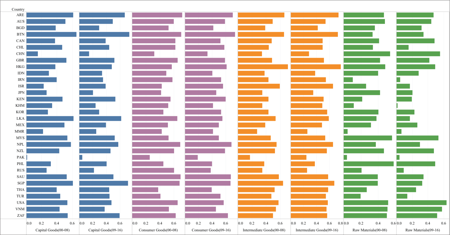
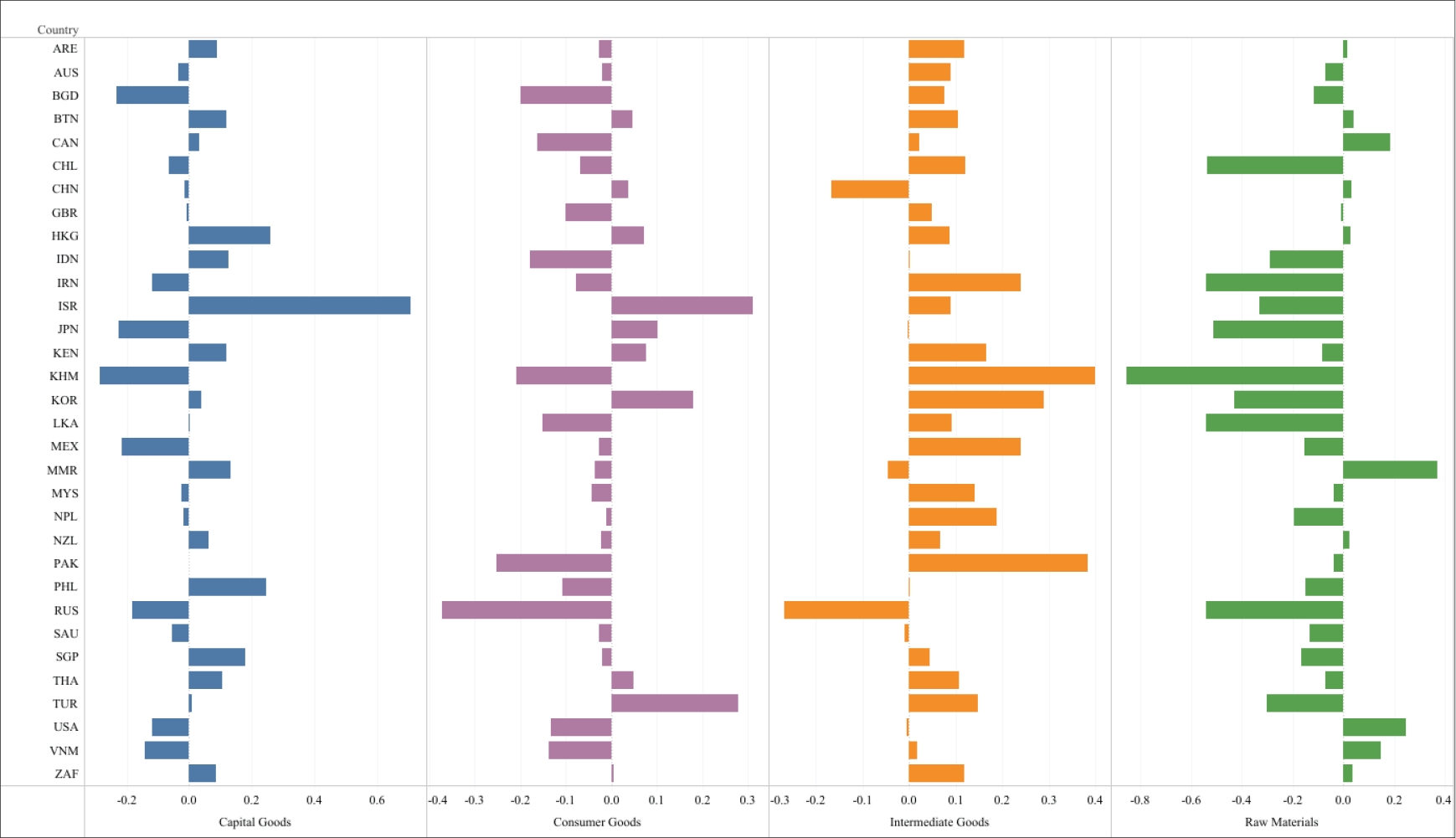
The TE of exports for all the sectors is shown in Figure 2. In order to create clear pictures of changes in TE over the two periods, adjusted TE ratios (ATER) are calculated in Figure 3. Both Figures 2 and 3 together provide an easier comparison of TE across countries, time periods and sectors. The estimation results show that India’s TE across countries and sectors lies within 80 per cent of potential. Exports with some countries in certain sectors exhibit low TE explaining India’s substantial export potential in such sectors. For RM, TE of export has decreased for most of the major trading partners except in instances like the USA, Canada and Vietnam. TE of export for Chile, Sri Lanka and Russia have drastically declined. India has the maximum export potential with Pakistan, Cambodia and Iran in RM sector. For IG, TE has increased for almost all the major trading partners except in instances like China and Japan. India has the best export performance for Bhutan, Hong Kong, UAE and Singapore. India has the maximum export potential with China, Russia and Myanmar in IG sector. TE of export has mixed results for CoG and CaG. For CoG, TE of export for Turkey, Republic of Korea and Israel have significantly improved whereas those of Russia, Canada and Cambodia have drastically declined. India has the maximum export potential with Pakistan, China and Thailand. For CaG, TE of export for UAE, Israel, Republic of Korea and Singapore have significantly improved whereas those of Mexico, Vietnam, Bangladesh and Cambodia have drastically declined. India has the maximum export potential with China, Pakistan, Japan and Indonesia.

Figure 2.

Source: The authors.

Figure 3.

Source: The authors.

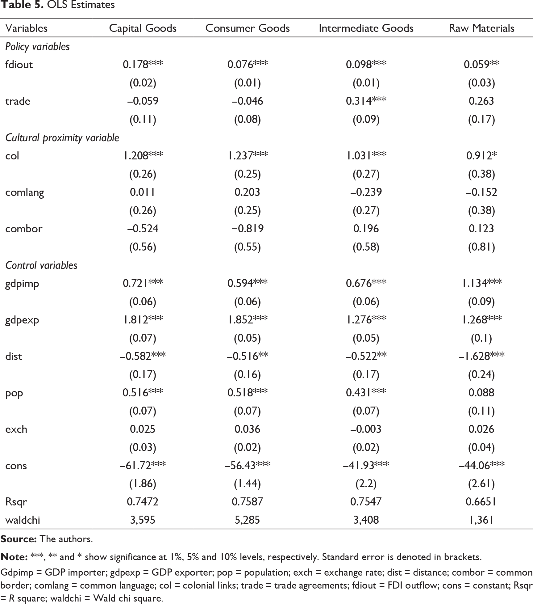
In summary, all the analyses show theoretical consistency with the gravity model estimation for SFA as well as OLS methods. Distance is one of the most important determinants for RM. Colonial links is one of the most important determinants for CoG and CaG. Trade agreements show ambiguous effects for all the sectoral analysis except IG. Trade liberalization in IG will lead to production rationalization across regions leading to increased exports potential. There are no statistically significant results for bilateral exchange rates. These results are in line with the results of Rangarajan and Kannan (2017) for Indian exports. FDI is one of the key determinants for CaG. The estimation results for TE of export shows a positive trend for IG, negative for RM and mixed for CoG and CaG. The export potential is the highest for RM, and export performance is the best for IG.

Conclusion and Implications

The study highlights the cultural and policy determinants for better export performance and competitiveness for different sectors. Trade agreements have an ambiguous effect on different sectors except for IG. Indian exporters have been unable to utilize these trade agreements due to lack of information, high administrative costs and prevalent non-tariff barriers. The findings for FDI highlights the positive effects of technological capacity building, market creation and improved supply chain performance for firms in the global market in the IG sector. In terms of export competitiveness, IG show an increase in overall TE but with marginal change share in exports. In contrast to this, the share in exports of CoG has improved over the years, but the increase in TE has been limited to certain countries only. This pattern explains that there has been a concentration of exports to certain countries only for CoG while better integration in the global value chain for IG. Therefore, India needs to focus on several fronts like diversifying the export basket across destinations and intra-regional trade cooperation, especially in Asia Pacific region to meet its potential. The findings on trade efficiency of exports give a comparative assessment of export competitiveness for all the four sectors. India has the highest export competitiveness for IG and the highest export potential for RM.

This study underscores several insights. First, it is important to create channels for information dissemination and reduction in communication costs involved for exports. Second, there is a need to accommodate the issues of non-tariff barriers in trade agreements, especially for the RM sector. Third, policy emphasis should be on building better forward and backward linkages to facilitate trade creation, especially for CoG and CaG. Fourth, there is a need for higher infrastructure spending in order to reduce trade costs. The role of infrastructure, institutional efficiency and political alignment are crucial for trade creation. The insignificant results for common border and low TE for neighbourhood countries underline the need to lower the trade costs and restrictions. Trade agreements show positive results only for IG, highlighting the need to formulate bilateral and multilateral agreements keeping in view the progress in other sectors. The positive results for FDI reaffirm the fact that policies need to focus on making the norms easier for financial flow across countries. Furthermore, one managerial implication is that businesses should increase financial flows in order to improve exports. Future work may investigate the firm-specific factors, which affect the export competitiveness at different stages of processing.

Footnotes

Acknowledgements

The authors are grateful to the anonymous referees of the journal for their extremely useful suggestions to improve the quality of the article. Usual disclaimers apply.

Declaration of Conflicting Interests

The authors declared no potential conflicts of interest with respect to the research, authorship and/or publication of this article.

Funding

The authors received no financial support for the research, authorship and/or publication of this article.

References

Aigner

Lovell

C. K.

Schmidt

(1977). Formulation and estimation of stochastic frontier production function models. Journal of Econometrics , 6(1), 21–37.

Anderson

J. E.

(1979). A theoretical foundation for the gravity equation. The American Economic Review , 69(1), 106–116.

Anderson

J. E.

Van Wincoop

(2003). Gravity with gravitas: A solution to the border puzzle. American Economic Review , 93(1), 170–192.

Armstrong

Drysdale

Kalirajan

(2008). Asian trade structures and trade potential: An initial analysis of South and East Asian trade. (EABER Working Paper 32). Australian National University, Canberra.

Athukorala

P. C.

(2009). The rise of China and East Asian export performance: Is the crowding-out fear warranted. World Economy , 32(2), 234–266.

Atif

R. M.

Haiyun

Mahmood

(2017). Pakistan’s agricultural exports, determinants and its potential: An application of stochastic frontier gravity model. The Journal of International Trade & Economic Development , 26(3), 257–276.

Baier

S. L.

Bergstrand

J. H.

(2009). Bonus vetus OLS: A simple method for approximating international trade-cost effects using the gravity equation. Journal of International Economics , 77(1), 77–85.

Battese

G. E.

Coelli

T. J.

(1995). A model for technical inefficiency effects in a stochastic frontier production function for panel data. Empirical Economics , 20(2), 325–332.

Bauer

P. W.

Berger

A. N.

Ferrier

G. D.

Humphrey

D. B.

(1998). Consistency conditions for regulatory analysis of financial institutions: A comparison of frontier efficiency methods. Journal of Economics and Business , 50(2), 85–114.

10.

Bergstrand

J. H.

(1985). The gravity equation in international trade: Some microeconomic foundations and empirical evidence. The Review of Economics and Statistics , 67(3), 474–481.

11.

Bergstrand

J. H.

(1989). The generalized gravity equation, monopolistic competition, and the factor-proportions theory in international trade. The Review of Economics and Statistics , 71(1), 143–153.

12.

Bhagavan

(1985). Capital goods sector in India: Past and present trends and future prospects. Economic & Political Weekly , 20(10), 404–421.

13.

Brodzicki

Uminski

(2013). International trade relations of enterprises established in Poland’s regions: Gravity model panel estimation (Working Paper No. 001). Institute for Development, Poland.

14.

Carrere

(2006). Revisiting the effects of regional trade agreements on trade flows with proper specification of the gravity model. European Economic Review , 50(2), 223–247.

15.

Deardorff

A.V.

, (2011). Determinants of bilateral trade: Does gravity work in a neoclassical world. In Stern R.

(eds.), Comparative advantage, growth, and the gains from trade and globalization: A festschrift in honor of Alan V Deardorff . World Scientific, Singapore.

16.

Doan

T. N.

Xing

(2018). Trade efficiency, free trade agreements and rules of origin. Journal of Asian Economics , 55, 33–41.

17.

Eregha

P. B.

(2019). Exchange rate, uncertainty and foreign direct investment inflow in West African monetary zone. Global Business Review , 20(1), 1–12.

18.

Felbermayr

G. J.

Toubal

(2010). Cultural proximity and trade. European Economic Review , 54(2), 279–293.

19.

Filippini

Molini

(2003). The determinants of East Asian trade flows: A gravity equation approach. Journal of Asian Economics , 14(5), 695–711.

20.

Francis

(2011). A sectoral impact analysis of the ASEAN-India free trade agreement. Economic & Political Weekly , 46(2), 46–55.

21.

Frankel

Stein

Wei

S. J.

(1995). Trading blocs and the Americas: The natural, the unnatural, and the super-natural. Journal of Development Economics , 47(1), 61–95.

22.

Ghemawat

(2001). Distance still matters. Harvard Business Review , 79(8), 137–147.

23.

Gokmen

(2017). Clash of civilizations and the impact of cultural differences on trade. Journal of Development Economics , 127(C), 449–458.

24.

Guzman

Ocampo

J. A.

Stiglitz

J. E.

(2018). Real exchange rate policies for economic development. World Development , 110, 51–62.

25.

Head

Mayer

Ries

(2010). The erosion of colonial trade linkages after independence. Journal of International Economics , 81(1), 1–14.

26.

Helpman

Krugman

(2002). Market structure and foreign trade: Increasing returns, imperfect competition, and the international economy . Cambridge, MA: MIT Press.

27.

Isard

Peck

(1954). Location theory and international and interregional trade theory. The Quarterly Journal of Economics , 68(1), 97–114.

28.

Jain

(2017). Public sector enterprise disinvestment in India: Efficiency gains in a political context. Journal of Asian Economics , 53, 18–36.

29.

Kalirajan

(2007). Regional cooperation and bilateral trade flows: An empirical measurement of resistance. The International Trade Journal , 21(2), 85–107.

30.

Mahadevan

Gonemaituba

(2013). A note on soil erosion and the loss in crop production: Case study of Fiji’s ginger farms. Journal of the Asia Pacific Economy , 18(3), 502–511.

31.

Martínez-Zarzoso

Nowak-Lehmann

(2003). Augmented gravity model: An empirical application to Mercosur-European union trade flows. Journal of Applied Economics , 6(2), 291–316.

32.

McCallum

(1995). National borders matter: Canada-US regional trade patterns. The American Economic Review , 85(3), 615–623.

33.

McDonald

Robinson

Thierfelder

(2008). Asian growth and trade poles: India, China, and East and Southeast Asia. World Development , 36(2), 210–234.

34.

Mishra

A. K.

Gadhia

J. N.

Kubendran

Sahoo

(2015). Trade flows between India and other BRICS countries: An empirical analysis using gravity model. Global Business Review , 16(1), 107–122.

35.

Mohanty

Sethi

(2019). Does inward FDI lead to export performance in India? An empirical investigation. Global Business Review . doi:10.1177/0972150919832770.

36.

Pradhan

J. P.

(2004). The determinants of outward foreign direct investment: A firm-level analysis of Indian manufacturing. Oxford Development Studies , 32(4), 619–639.

37.

Rangarajan

Kannan

(2017). Determinants of India’s exports. Journal of Quantitative Economics , 15(3), 629–646.

38.

Ravishankar

Stack

M. M.

(2014). The gravity model and trade efficiency: A stochastic frontier analysis of Eastern European countries’ potential trade. The World Economy , 37(5), 690–704.

39.

Sanso

Cuairan

Sanz

(1993). Bilateral trade flows, the gravity equation, and functional form. The Review of Economics and Statistics , 75(2), 266–275.

40.

Seleka

T. B.

Kebakile

P. G.

(2017). Export competitiveness of Botswana’s beef industry. The International Trade Journal , 31(1), 76–101.

41.

Tinbergen

(1962). Shaping the world economy: Suggestions for an international economic policy . New York, NY: Twentieth Century Fund.

42.

Veeramani

(2007). Sources of India’s export growth in pre-and post-reform periods. Economic & Political Weekly , 42(25), 2419–2427.