FX Volatility Impact on Indian Stock Market: An Empirical Investigation

Abstract

Examining the interrelationship between currency market volatility and stock market volatility will create abundant trading opportunities to the investors irrespective of whether the return of one market is moving up or down. This research work intended to examine how the exchange rate volatility between Indian rupee and foreign currencies, such as US dollar, euro, Japanese yen and British pound, can influence the return and volatility of the Indian stock market. The research data extensively cover daily price observations of foreign currencies as well as Nifty index for 1500 days. The generalized autoregressive conditional heteroskedasticity (GARCH) is used for modelling foreign exchange (FX) rates volatility and its impact across Indian stock market. The mean equation of the model confirms that any appreciation in Indian rupee will lead to channelization of more funds towards stock market. Further, it is validated that the volatility shocks between the stock market and currency market are quite persistent. Besides the model also points that the volatility attributes are very strong between US dollar and Nifty. The Granger causality test wrap up with a finding that the volatility shocks of British pound have a causal relation with Nifty return. The result of this study will help the domestic as well as foreign investors in favour of portfolio diversification decisions. The study also spots that the policymakers can indirectly intervene into stock market through monitory policy measures.

Keywords

FX Volatility Nifty Return Granger Causality Test Generalized Autoregressive Conditional Heteroskedasticity

Introduction

This research empirically examines the foreign exchange (FX) volatility impact on the National Stock Exchange (NSE) of India. The exchange rate between currencies is a matter of concern for various players, such as traders, governments, corporate, banks, investment funds, etc. The exchange rate fluctuations of currencies directly or indirectly influence stock market return. For instance, the investors holding foreign equity will be naturally exposed to FX rate fluctuations. As far as such investments are concerned, the equity return as well as currency return has become a matter of concern for shaping their decision. As per ‘portfolio balance approach’ proposed by Frankel and Rodriguez (1975), a flourishing stock market would attract capital flows from foreign investors, which may cause an increase in the demand for domestic currency. The reverse would happen in case of falling stock market where the investors would try to sell their stocks to avoid further losses and would convert their money into foreign currency. As a result, rising stock prices would lead to an appreciation in exchange rates, and fall in stock price leads to exchange rate depreciation. From the angle of ‘goods and market approach’ proposed by Dornbusch and Fischer (1980), a depreciation of the local currency makes exporting goods attractive and leads to an increase in foreign demand and revenue for the firm; as a result, the firms value and the stock prices will appreciated. On the other hand, an appreciation of the local currency decreases profits for an exporting firm because it leads to a decrease in foreign demand of its products, as a result the stock prices also decreased. The above theories are explaining the relationship between exchange rate fluctuation and stock market return in two angles.

Considering the above theories, the scenario can be reiterated from the angle of domestic investors. Say a domestic investor is considering stock as well as foreign currencies in his portfolio. If the stock market is outperforming; the investor tends to withdraw his investment from foreign currency market and more fund will be channelized towards stock market. Ultimately, withdrawal from foreign currency may lead to appreciation of domestic currency. If stock return is not promising; the investors will force to transfer their investment from stock market to foreign currency market. This may lead to increase in the demand for foreign currency and consequently result in depreciation of domestic currency. A balanced portfolio consisting of stock and currencies would enable the investors to hedge effectively their position by transferring from one investment option to another.

In recent years, foreign currencies are considered as an important investment avenue by various traders, mutual fund companies and portfolio managers. This in fact created a need for understanding the linkage between FX fluctuations and its impact in stock market. But theoretically, several extraneous factors, such as interest rate, inflation rate, money supply, price levels, etc., can also contribute to exchange rate between currencies. Rather than the above extraneous factors, understanding the direct linkage between exchange rates and stock market performance would enable the stock advisors to suggest appropriate measures to address the exchange rate-related issues. This work is investigating the volatility effect of four actively traded currencies, namely, US dollar (USD), euro (EUR), Japanese yen (JPY) and Great British pound (GBP), on Indian stock market.

Review of Literature

The linkage between the exchange rates and stock market returns had been subject to extensive research. Theoretically, rising stock prices would lead to an appreciation in exchange rates and fall in stock price leads to exchange rate depreciation (Frankel & Rodriguez, 1975). As a result, there exists a negative relation between stock return and exchange rate volatility. Adjasi, Harvey and Agyapong (2008) established a relationship with exchange rate volatility and stock market return in Ghana. They found that there exist a negative relationship between exchange rate volatility and stock market return. A study carried out by Agrawal, Srivastav, and Srivastava (2010) analyzes the relationship between rupee–USD exchange rate and Nifty returns. A negative correlation between Nifty returns and exchange rates was observed. A research work by Kutty (2010) examines the connection between stock price and exchange rate in Mexico. The researcher concludes that in short run there exist relationship between stock prices and exchange rates. But such evidence is absent in long run. Ahmadi, Rezayi and Zakeri (2012) observes the exchange rate volatility and its intervention in stocks of selected companies listed with Tehran Stock Exchange. Using Glosten, Jagannathan, and Runkle-Model (GRJ) generalized autoregressive conditional heteroskedasticity (GRJ-GARCH) model, they found strong evidence of exchange rate exposure on stock market. Mlabo, Maredza, and Sibanda (2013) assessed the effect of currency volatility in Johannesburg Stock Exchange. The study signals a weak relationship between stock market volatility and currency exchange rate. Hajilee and Nasser (2014) examined the effect of exchange rate uncertainty on stock market development for 12 emerging economies over the period 1980–2010. The research concludes that exchange rate volatility has a significant effect on stock market development in both the short run and long run in a majority of countries. In another study, Frederick, Muasya and Kipyego (2014) have established that there was a strong, positive correlation between FX rates represented by the Kenyan shilling to the USD and the stock price index as provided by the Nairobi Securities Exchange 20-share index. Therefore, when the exchange rate ‘increases’, it implies an increase of the Kenya shilling or appreciation of the foreign currency. Lawal and Ijirshar (2015) analyze the exchange rate volatility and Nigerian stock market performance. GARCH model shows that exchange rate and inflation rate have impacted negatively on the growth of Nigerian stock market. All the above studies were conducted in different context and in different periods. But the result of these works confirmed the well-established association between exchange rate fluctuation and stock returns.

Some recent studies also examined the relationship between exchange rate fluctuations and stock market returns. Najaf and Najaf (2016) identified a unidirectional relationship between Nifty returns and exchange rates. Yadav (2016) states that negative correlation existed among the stock market returns and exchange rate in India; however, the degree of correlation was not very significant. Ngan (2016) in his study states that fluctuation in FX rate VND/USD causes the change in stock prices of commercial joint stock banks in Vietnam. On the opposite way, the change in stock price does not cause the change in FX rate; this relation is one-way relation. Sichoongwe (2016) also found that there is a negative relationship between exchange rate volatility and stock market returns in Zambia. This relation was further confirmed by another study conducted in 21 emerging market economies (Akdogu & Birkan, 2016). Rafiq and Hasan (2016) confirmed a short-run relationship between exchange rate and stock prices by examining the context of Pakistan economy. The short-run relation between these variables in Turkish economy was further confirmed by Mwambuli and Xianzhi (2016). From the recent literature, we may arrive at a conclusion that in short run the relation between stock price and FX fluctuation is evident.

Kennedy and Nourzad (2016) found that the 9/11 terrorist attack, bear markets, fluctuations in jobless claims and negative equity market returns increase financial volatility. Using GARCH (1,1) model, it is found that when major drivers of financial volatility are controlled, increased exchange rate volatility exerts a positive and statistically significant effect on the volatility of stock returns.

It is quite interesting to examine how domestic currency appreciation/depreciation are influencing stock returns. Hypothetically, currency appreciation and stock market performance are interconnected and currency depreciation may lead to stock market clash. Domestic currency depreciation and its uncertainty adversely affect stock market returns across countries (Fang & Miller, 2002). In this context, it is argued that after local currency appreciation, ‘hot money’ flowing from foreign funds into the local markets followed by local investors’ speculations on markets pushed the market into a high level based on the expectation of the local currency’s further appreciation (Tian & Ma, 2009). In another research, Dimitrova (2005) used multivariate, open-economy, short-run model that allows for simultaneous equilibrium in the goods, money, FX and stock markets in USA and the UK over 14 years. The study result interestingly shows that currency depreciation may depress the stock market. The above studies justify the theoretical arguments of currency appreciation/depreciation on stock market returns.

Other than exchange rate, several other factors may cause fluctuation in stock price. The variation in stock price causes due to such extraneous factor can be called as spillover effect. Apte (2001) investigated the volatility of stock market and the nominal exchange rate in India. The Exponential Generalized Autoregressive Conditional Heteroskedasticity (EGARCH) model states that major market indices in India support the two-way linkage of exchange rates on stock returns. But with respect to other indices, it shows spillover effect from forex market to stock market. They conclude that the macro-economic factors, such as interest rates, consumer price index, etc., can impact stock market volatility. This modelling compromises very much with the view point of Hodrick (1990). He argues that the market fundamentals can cause variance in expected return and the conditional variance of asset prices. Choi, Fang and Fiu (2009) examines volatility spillovers between stock market returns and exchange rate changes within the New Zealand economy. The results show that the NZ market is exposed to foreign currency movements. Jebran and Iqbal (2016) examine volatility spillover effects between stock market and FX market in selected Asian countries, such as Pakistan, India, Sri Lanka, China, Hong Kong and Japan. The outcome of the analysis shows bidirectional asymmetric volatility spillover between stock market and FX market of Pakistan, China, Hong Kong and Sri Lanka. While in India, the results reveal unidirectional transmission of volatility from stock market to FX market.

Aim and Scope

The study was conducted with the following objectives:

To test whether the exchange rate fluctuations between Indian rupee and foreign currencies can be used for predicting stock market return.

To develop a model for observing how the exchange rate volatility between Indian rupee and foreign currencies, such as USD, EUR, JPY and GBP, can influence the return and volatility of Indian stock market.

The exchange rate returns of four actively traded currencies, namely USD, EUR, GBP and JPY, to INR and Nifty return were the natural choice of inclusion of this study, as these variables are widely used by the market participants for benchmarking. The study result will serve different stakeholders to enlarge their insights dealings with forex market and stock market. As far as the domestic investors are concerned a well-established knowledge on stock market and currency market will enable them to hedge their investment portfolio through proper channelization. The stock fluctuation as well as currency fluctuation has become a matter of concern for foreign portfolio investors. Proper modelling using above variables will help them to arrive at appropriate decision. The result of this study will also help the policymakers to check and correct the deviations observed through frequent market intervention.

Hypotheses

The entire study is developed on the basis of the following assumptions.

H1: The FX return series data of USD, EUR, JPY and GBP to INR are normally distributed.

H2: The time series return data (USD, EUR, JPY, GBP and NSE) used for mathematical modelling are not stationary.

H3: The FX volatility between INR and USD, EUR, JPY and GBP cannot root NSE return.

H4: There does not exist any Autoregressive Conditional Heteroskedasticity (ARCH) effect on the FX volatility impact to NSE return.

Data and Methodology

The daily exchange rate variations of USD, EUR, JPY and GBP to Indian rupee for the study period were collected from www.investing.com. Likewise, nifty movement was obtained from www.nseindia.com. This pragmatic study extensively covers daily movements of 1500 days starting from 17 December 2009 to 31 December 2015, for the reason that these years are considered to be the most recent normal periods when this research starts. The study period was fixed purely on judgemental basis. Later data processing was performed through the following stages. Initially, log returns of exchange rates and Nifty were computed in Microsoft excel using the following formula,

R = L n (P 1 / P 0)

(1)

In the above equation, R denotes return, P1 stands for current day’s price and P0 stands for price of the previous day. Through Ln, we assume that the returns are log normally distributed.

The formula generated 1499 daily returns data each for FX rates and Nifty. Further, the computed returns data were entered in EViews 9.SV.statistical package under appropriate headings. The initial attempt was to check whether the collected time series data are stationary, because only stationary data series will ensure constant statistical properties in past and future. Moreover, a stationary time series is found to be fit for future data modelling. Augmented Dickey Fuller (ADF) test was used for examining whether the collected time series are stationarized or not. Then causality test was performed for checking whether FX rates are good for predicting future stock returns. Causality of FX rates variations on Nifty return was observed using Granger causality test in VAR environment. In order to examine how FX rates are influencing stock market return and to observe the randomly varying volatility effect, a GARCH (1,1) model was developed.

Empirical Analysis and Discussions

The analysis part consists of checking stationarity of the time series, investigating the causality of variation in FX rates on stock market returns, diagnostic tests and developing GARCH (1,1) model.

Descriptive Statistics

The results from descriptive statistics are reported in Table 1. It also provides an outlook on the normality test performed for developing the volatility model.

From Table 1, it is clear that the USD to INR obtained an average daily return of 0.003 per cent during the study period with a maximum of 3.49 per cent and with a minimum of –4.74 per cent. It is also examined that EUR to INR provides only a daily return of 0.001 per cent. The maximum positive daily return generated by EUR to INR was 3.34 per cent and the minimum return was –5.04 per cent. JPY generated an average daily return of 0.005 per cent to INR during the study period. With respect to GBP, a mean daily return of 0.002 per cent was reported. The corresponding volatilities measured by standard deviation were uniform for all currencies during the study period. The return series for USD and JPY reported to have a negative skewness of –0.036 and –0.006, respectively, suggesting that these distributions have long left tail. The return distribution of EUR and GBP exhibited a positive skewness with values of 0.185 and 0.003. From the above, we have to examine the normality of residuals on the assumption that the residuals are normally distributed, because normal GARCH model will reduce the chance of volatility huddles. Here, Jarque–Bera test is used to examine whether sample data have the skewness and kurtosis matching to a normal distribution. Normality test was performed on postulation that the return series are normally distributed. Table 1 gives clear evidence that the probability values obtained for all return series in Jarque–Bera test are statistically significant at 5 percentage level of significance (p-values 0.00 < 0.05). This leads to rejection of null hypotheses by accepting the fact that the return series are not normally distributed (H1: Null hypothesis is rejected).

Table 1.

Descriptive Statistics & Normality Test

Descriptive Statistics	USD	EUR	JPY	GBP
Mean	0.003	0.001	0.005	0.002
Median	0.010	–0.019	0.023	–0.027
Maximum	3.496	3.340	3.628	3.341
Minimum	–4.739	–5.047	–4.033	–4.484
Std. Dev.	1.000	1.000	1.000	1.000
Skewness	–0.036	0.185	–0.006	0.003
Kurtosis	3.615	3.764	3.538	3.615
Jarque-Bera	23.926	36.530	18.126	23.630
Probability (J-B)	0.000	0.000	0.000	0.000

Source: Processed data.

Augmented Dickey Fuller (ADF) Test

Testing unit root has become a concern for econometric modelling and forecasting. This research followed the statistical model suggested by Dickey and Fuller (1979, 1981) and by Dickey and Said (1984) for checking stationarity of the collected time series data. This empirical analysis is conducted based on the assumption that the time series data used for mathematical modelling are not stationary. Stationary time series are those which the statistical properties will remain constant over a period of time. If the series is stationary, it is understood that its statistical properties will be the same in the future as they have been in the past. It is also interesting to check whether the shocks in the collected data have permanent or transitory effect. This study used an improved version of the Dickey–Fuller test for a larger and more complicated set of time series models.

\begin{matrix} Δ y_{t} = α + β t + γ y_{t - 1} + δ_{1} Δ y_{t - 1} + ... + \\ δ_{p - 1} Δ y_{t - p + 1} + ε_{t}, \end{matrix}

(2)

where Y_t represents time series to be tested, α is a constant, β the coefficient on a time trend and p the lag order of the autoregressive process and ε_t is the white noise error term. Imposing the constraints α = 0 and β = 0 corresponds to modelling a random walk and using the constraint β = 0 corresponds to modelling a random walk with a drift. The test is usually carried out on the assumption that ‘the time series data is not stationary’. If the test statistics is found to be negative number, the chance for rejection of null hypotheses is higher. The results obtained in Augmented Dickey Fuller Test are presented in Table 2.

Table 2.

Augmented Dickey Fuller Test

Return Data	T-Statistics	Coefficient	SE	P-value*	Critical Values
Return Data	T-Statistics	Coefficient	SE	P-value*	1%	5%	10%
USD	–29.224	–1.051	0.036	0.000
EUR	–40.067	–1.035	0.026	0.000
JPY	–38.727	–1.002	0.026	0.000	–3.435	–2.863	–2.567
GBP	–40.008	–1.033	0.026	0.000
NSE	–36.149	–0.933	0.026	0.000

Source: Processed data.

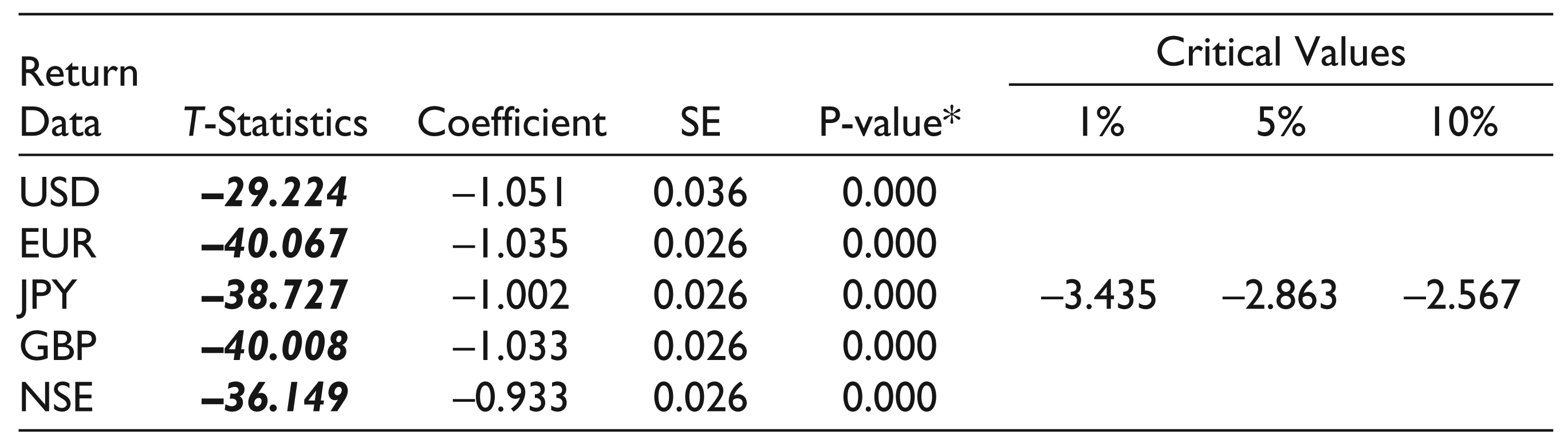
The test results produced values of –29.224, –40.067, –38.727, –40.008 and –36.149, respectively, for the time series return data of USD, EUR, JPY, GBP and NSE. The above values are much behind the critical values of –3.435, –2.863 and –2.567, respectively, at 1 per cent, 5 per cent and 10 per cent levels of significance. So it can be inferred that the test statistics are falling behind critical values at 1 per cent, 5 per cent and 10 per cent, respectively. Thereby ADF results point towards the evidence of stationarity in the selected time series. Moreover, the probability values obtained (p-value = 0.000) for the test statistics are much below the critical values of 0.01, 0.05 and 0.1. This again points that the time series return data of USD, EUR, JPY, GBP and NSE are stationary. (H2: Null hypothesis is rejected).

Granger Causality Test

Granger causality test investigates the ability to predict the future values of a time series using prior values of another time series. This statistical hypothesis test was first proposed in 1969 by Clive Granger. In economics, this is a widely used tool for measuring the usefulness of a time series data in forecasting another time series. The essential pre-condition for applying Granger causality test is to ascertain the stationarity of the variables in the pair. A time series is said to Granger-cause of another if it can be shown, usually through a series of t-tests and F-tests on lagged values, and values of the former provide statistically significant information about future values of the later. Another requirement for the Granger causality test is to find out the appropriate lag length for each pair of variables. For this purpose, the researcher used the vector auto regression (VAR) lag order selection method. This mechanism was employed on the ground that Granger causality test is found to be well specified if they are applied in standard VAR form (MacDonald & Kearney, 1987; Miller & Russek, 1990; Lyons & Murinde, 1994).

For instance, to solve this mathematically, I followed the below equations. In a stationary time series of two data set, namely, x and y, first I computed the proper lagged values of y to include in a univariate auto-regression of y.

y_{t} = a_{0} + a_{1} y_{t - 1} + a_{2} y_{t - 2} + ... + a_{m} y_{t - m} + e r r o r_{t} .

(3)

Next, the auto-regression is augmented by including lagged values of x,

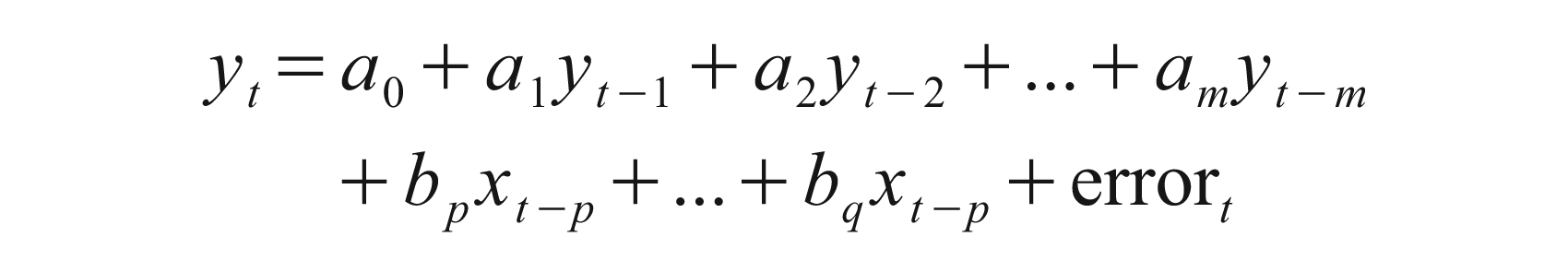
\begin{matrix} y_{t} = a_{0} + a_{1} y_{t - 1} + a_{2} y_{t - 2} + ... + a_{m} y_{t - m} \\ + b ​_{p} x_{t - p} + ... + b ​_{q} x_{t - p} + e r r o r_{t} \end{matrix}

(4)

For the above, ‘x’ is independent time series and ‘y’ is dependent time series. In this research, Granger causality test has performed under VAR environment. Here, two lag intervals for endogenous were fixed based on the lag selection criteria. This was carried out to ensure standardization for the time series data distribution. The NSE return is considered as the dependent variable and FX volatility considered as the independent variables. Table 3 exhibits the result of Granger causality test performed under VAR environment using Eviews statistical package.

Table 3.

Granger Causality Test in VAR Environment

Independent Variables	Chi-square	df	Prob.*
USD	2.984	2	0.225
EUR	0.899	2	0.638
JPY	1.676	2	0.433
GBP	6.317	2	0.043
All	9.922	8	0.271

Source: Processed data.

Note: Dependant variable: NSE.

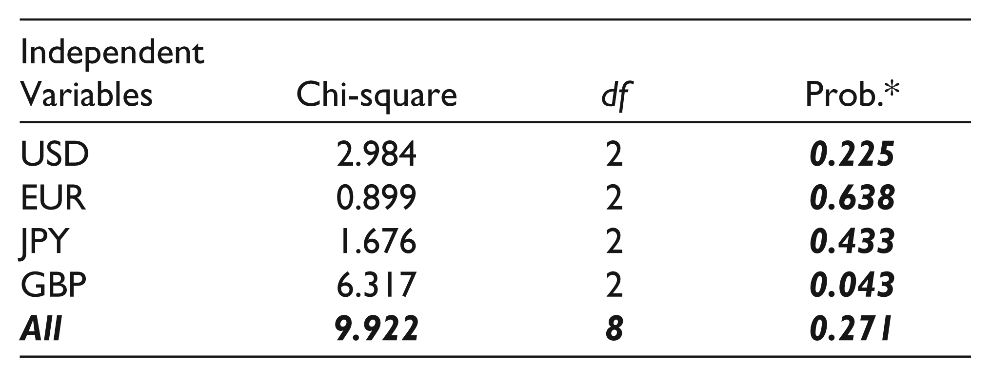
This test was performed with the assumption that FX volatility factor does not cause the stock market return. The exchange rate impact of four currencies, namely, USD, EUR, JPY and GBP, were tested on NSE return to analyze the results. At 5 per cent level of significance, the test statistics produced a combined p-value of 0.271 (chi-square = 9.92) which is much higher than that of the critical value 0.05. Hence, it can be inferred that the FX volatility factors cannot cause NSE return (H3: Null hypotheses accepted). While observing the Granger causality result independently with respect to USD, a chi-square value of 2.984 is obtained with a probability value of 0.225 (p-value > 0.05). For EUR and JPY, chi-square values of 0.899 and 1.676 obtained, respectively, with probability values of 0.638 and 0.433 at 5 per cent level of significance. In all the above cases, we have to accept the null hypotheses on the ground that the obtained probability values are much above the critical value of 0.05. So, we have to conclude that the volatility factors of USD, EUR and JPY cannot root NSE return. But interestingly, the probability value 0.043 (p-value < 0.05) of GBP turns out to be significant at 95 per cent confidence level. This is pointing towards rejection of null hypotheses and thereby we could arrive at an assumption that GBP volatility factor does cause fluctuation in NSE return. This discrepancy observed in the result of Granger causality test among exchange rates really motivated to develop a GARCH (1,1) model.

Heteroskedasticity Test

One of the assumptions of the classical linear regression model is that there is no heteroskedasticity. In order to check the manifestation of heteroskedasticity in residuals, ARCH test was conducted with the hypothecation of ‘there is no ARCH effect’. Table 4 exhibits the results of ARCH test.

Table 4.

Heteroskedasticity Test

	F-statistics	Observed R-squared	F test p-value	Chi-square p-value
USD	2.0376	2.0376	0.1537	0.1535
EUR	3.6014	3.5475	0.0579	0.0579
JPY	1.3252	1.3258	0.2498	0.2495
GBP	3.8350	3.8301	0.0504	0.0504

Source: Processed data.

The probability values of F-test statistics on volatility effect of USD, EUR and JPY are 0.1537, 0.0579 and 0.2498; falling above the critical value of 0.05 at 95 per cent confidence level. Here, the null hypotheses will be accepted as the test statistics produced strong evidence that there is no ARCH effect (H4: Null hypothesis is accepted). With respect to the effect of GBP; the test statistics is fairly above the critical value (0.0504 > 0.05). Hence, it can also be inferred that there is no ARCH effect with respect to the stimulus of GBP on NSE returns.

Correlogram-squared Residual Test

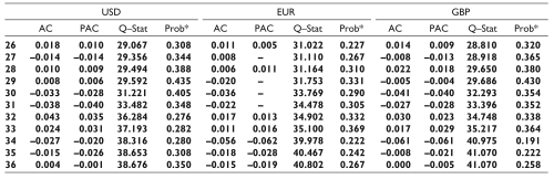
Auto correlation effects of FX returns were examined by fixing 36 lag intervals. The fixation of lag intervals was based on the model proposed by Ivanov and Kilian (2005). The detailed result of autocorrelation with 36 lag periods is presented in Table 5. If the probability of correlogram of residuals squared under ‘Q’ statistics is above 0.05 then it is presumed that there does not exist any serial correlation. From Table 5, it is clear that the autocorrelation effect does not stay alive in the above models. Because the probability values obtained for Q-statistics (p-values > 0.05) is much above the critical value of 0.05 at 5 per cent level of significance.

Table 5.

Auto Correlation

	USD				EUR				GBP
	AC	PAC	Q–Stat	Prob*	AC	PAC	Q–Stat	Prob*	AC	PAC	Q–Stat	Prob*
1	–0.037	–0.037	2.0423	0.153	–0.049	–	3.6072	0.058	–0.051	–0.051	3.8393	0.050
2	–0.030	–0.031	3.3630	0.186	–0.010	–	3.7727	0.152	–0.015	–0.017	4.1680	0.124
3	0.044	0.042	6.3242	0.097	0.010	0.009	3.9154	0.271	0.045	0.043	7.1820	0.066
4	–0.007	–0.004	6.3926	0.172	–0.012	–	4.1475	0.386	–0.023	–0.019	8.0051	0.091
5	–0.069	–0.067	13.567	0.019	–0.045	–	7.1437	0.210	–0.052	–0.053	12.020	0.035
6	0.056	0.049	18.334	0.005	0.043	0.039	9.9658	0.126	0.028	0.020	13.205	0.040
7	0.006	0.006	18.382	0.010	0.057	0.061	14.930	0.037	0.043	0.046	15.946	0.026
8	0.007	0.016	18.450	0.018	–0.019	–	15.483	0.050	–0.004	0.005	15.969	0.043
9	–0.009	–0.013	18.579	0.029	0.057	0.055	20.330	0.016	0.026	0.023	17.023	0.048
10	0.016	0.011	18.959	0.041	0.012	0.015	20.544	0.025	0.018	0.016	17.521	0.064
11	–0.016	–0.009	19.334	0.055	–0.011	–	20.737	0.036	–0.012	–0.005	17.742	0.088
12	0.029	0.028	20.573	0.057	–0.002	0.000	20.740	0.054	0.016	0.018	18.136	0.112
13	–0.025	–0.024	21.485	0.064	–0.017	–	21.160	0.070	–0.011	–0.012	18.319	0.146
14	0.011	0.010	21.672	0.086	0.003	0.004	21.173	0.097	0.008	0.009	18.414	0.189
15	0.011	0.011	21.853	0.112	–0.015	–	21.506	0.121	–0.028	–0.029	19.604	0.188
16	–0.003	–0.002	21.864	0.148	0.037	0.027	23.555	0.100	0.016	0.011	19.995	0.220
17	–0.012	–0.008	22.093	0.181	–0.008	–	23.644	0.129	–0.002	–0.002	19.999	0.274
18	0.020	0.012	22.713	0.202	0.015	0.012	23.974	0.156	0.019	0.020	20.533	0.304
19	0.015	0.020	23.061	0.235	0.000	0.001	23.975	0.197	0.005	0.004	20.572	0.361
20	0.048	0.051	26.524	0.149	0.050	0.053	27.730	0.116	0.061	0.062	26.305	0.156
21	–0.005	–0.002	26.561	0.186	–0.017	–	28.159	0.136	–0.018	–0.012	26.795	0.178
22	–0.023	–0.026	27.391	0.197	–0.038	–	30.385	0.109	–0.024	–0.022	27.676	0.187
23	–0.004	–0.005	27.412	0.239	–0.006	–	30.439	0.137	–0.011	–0.018	27.865	0.221
24	–0.026	–0.027	28.428	0.242	–0.012	–	30.660	0.164	–0.015	–0.013	28.231	0.250
25	0.010	0.016	28.595	0.281	0.011	0.009	30.829	0.195	0.014	0.018	28.510	0.285
26	0.018	0.010	29.067	0.308	0.011	0.005	31.022	0.227	0.014	0.009	28.810	0.320
27	–0.014	–0.014	29.356	0.344	0.008	–	31.110	0.267	–0.008	–0.013	28.918	0.365
28	0.010	0.009	29.494	0.388	0.006	0.011	31.164	0.310	0.022	0.018	29.650	0.380
29	0.008	0.006	29.592	0.435	–0.020	–	31.753	0.331	–0.005	–0.004	29.686	0.430
30	–0.033	–0.028	31.221	0.405	–0.036	–	33.769	0.290	–0.041	–0.040	32.293	0.354
31	–0.038	–0.040	33.482	0.348	–0.022	–	34.478	0.305	–0.027	–0.028	33.396	0.352
32	0.043	0.035	36.284	0.276	0.017	0.013	34.902	0.332	0.030	0.023	34.748	0.338
33	0.024	0.031	37.193	0.282	0.011	0.016	35.100	0.369	0.017	0.029	35.217	0.364
34	–0.027	–0.020	38.316	0.280	–0.056	–0.062	39.978	0.222	–0.061	–0.061	40.975	0.191
35	–0.015	–0.026	38.653	0.308	–0.018	–0.028	40.467	0.242	–0.008	–0.021	41.070	0.222
36	0.004	–0.001	38.676	0.350	–0.015	–0.019	40.802	0.267	0.000	–0.005	41.070	0.258

The GARCH (1,1) model developed after considering the diagnostic test results, such as correlogram-squared residual test, normality test and heteroskedasticity test. From the diagnostic tests, we obtained results, such as there is no autocorrelation and the ARCH effect was not present. These signs are good for developing the model while normality test shows that the residuals are not normally distributed. By circumventing the normality test results, we can proceed for developing a GARCH (1,1) model on account of considering the diagnostic outcomes derived from correlogram and ARCH test results.

FX Volatility Impact on NSE Return: GARCH (1,1) Model

Model Description

GARCH model is an extension of ARCH model and was first developed by Bollerslev (1986). GARCH (1,1) is a time series model that is becoming widely used in econometrics and finance to check the randomly varying volatility effect. The (1,1) in parentheses is a standard notation in which the first number refers to how many autoregressive lags, or ARCH terms, appear in the equation, while the second number refers to how many moving average lags are specified, which here is often called the number of GARCH terms.

GARCH model found to be useful for a wide range of capital market application (Gazda & Vyrost, 2003). Karmakar (2005) favoured GARCH (1,1) model on the ground of high persistence and predictability of volatility. Ahmed and Sulaiman (2011) state that GARCH (1,1) model is found to be useful for finding symmetry effect time series data. The predictability of GARCH model was further confirmed by Mlabo, Maredza and Zibanda (2013) in their study. In the words of Gokcan (2000) for emerging stock markets, GARCH (1,1) model performs better than EGARCH model, even if stock market return series display skewed distributions. The GARCH model and which error distribution to use are still open to question, especially where the model that best fits the in-sample data may not give the most effective out-of-sample volatility forecasting ability (Kosapattarapim, Lin & McCrae, 2012). GARCH and EGARCH approaches are found to be quite efficient in forecasting the exchange rate, MLFNN and NARX. Gupta and Kasyap (2016) employed GARCH family models for forecasting exchange rate volatility between GBP and INR. Alagidede and Ibrahim (2016) relied on the GARCH developed by Bollerslev (1986) not only because the exchange rate best follows the GARCH process but because it captures past values of the exchange rate as opposed to the ARCH. GARCH model allows having differential impacts on conditional variance of the past shocks (Liko & Kashuri, 2016).

GARCH (1,1) Model

A GARCH (1,1) model has two parts, namely, mean equation and variance equation. Here, the variance equation is developed on the basis of the residuals derived from mean equation.

D V R = C 1 + C 2 * I V R + e

(5)

\begin{matrix} H_{t} = C 3 + C 4 * R E S I D {(- 1)}_{}^{^}_{}^{2} + \\ C 5 * (G A R C H - 1) \end{matrix}

(6)

For the above model, DVR denotes return of dependent variable; CI, C2, C3, C4 and C5 are constants derived from this model and Ht is the variance of residual (error) derived from mean equation. It is the current return variance volatility of the dependent variable. IVR stands for the independent variables and ‘e’ denotes the error term. For this research, we can consider NSE return as the dependent variable and FX returns as the independent variables. The detailed modelling of the scenario using GARCH (1,1) is presented in Table 6.

Table 6.

GARCH (1,1) Model

	USD			EUR			JPY			GBP
	Coe.	Z–Value	Prob.	Coe.	Z–Value	Prob.	Coe.	Z–Value	Prob.	Coe.	Z–Value	Prob.
Return Equation
C (intercept)	0.00	2.54	0.01	0.00	2.08	0.04	0.00	1.77	0.08	0.00	2.18	0.03
AR(1) (ρ)	–0.82	–21.84	0.00	–0.40	–1.00	0.32	–0.47	–20.63	0.00	–0.47	–12.98	0.00
Variance Equation
C	0.00	2.68	0.01	0.00	2.74	0.01	0.00	2.68	0.01	0.00	2.71	0.01
RESID(–1)^2 (α)	0.05	5.59	0.00	0.06	5.93	0.00	0.04	4.64	0.00	0.05	5.43	0.00
GARCH (–1) (β)	0.94	73.91	0.00	0.92	59.22	0.00	0.94	69.91	0.00	0.94	73.46	0.00
α + β	0.99			0.98			0.98			0.95
R–squared		0.19			0.00			0.16			0.09
Adjusted R–squared		0.19			0.00			0.16			0.09
Log Likelihood		4885.8			4744.74			4863.02			4809.95
Durbin Watson sat.		1.97			1.87			1.96			1.93
Schwarz criterion		–6.49			–6.31			–6.46			–6.39
Akaike Info Cir.		–6.51			–6.32			–6.48			–6.41

Source: Processed data.

Note: Dependant variable: NSE.

This research focused to develop a model by checking how FX rate fluctuations are influencing the stock market returns. Table 6 exhibits the mean and variance obtained on the basis of using normal Gaussian distribution. In the mean equation, negative co-efficient values were obtained. This signals that there exists negative relation between FX rates and NSE return. For instance, the co-efficient of NSE return on USD is –0.82. This signals that an increase in USD return by one percentage leads to a decrease in NSE return by 0.82 percentage. Likewise, EUR, JPY and GBP also report negative return coefficients of –0.40, –0.47 and –0.47, respectively. The negative relation strongly spotting towards the fact that foreign currency investment is considered as a perfect alternative for stock market investment in India. This model suggests that more and more investors will be attracted to stock market while INR is appreciating. The findings of this study strongly supporting the theory proposed by Frankel and Rodriguez (1975). The above relation was further examined by means conducting a Z-test at 5 per cent level of significance. The results show that except EUR the p-value obtained for the co-efficient are statistically significant at 5 per cent level of significance. So, we may have to conclude that the volatility attributed to EUR return cannot influence stock return of NSE.

While examining the variance equation the excess return attribute by FX rates to NSE is 0.05, 0.06, 0.04 and 0.05, respectively, for USD, EUR, JPY and GBP. Further Z-value of these variance results signifies that there exist ARCH effect as p-values obtained for α (RESID (–1)²) is falling within the significance level of 5 per cent (p-values 0.000 < 0.05). The ARCH effect assumes that there exists volatility clustering. In the words of Mandelbrot (1963), volatility clustering refers that ‘large changes tend to be followed by large changes, of either sign, and small changes tend to be followed by small changes’. Whereas looking at GARCH effect, the obtained β coefficients for the variance equation was 0.94, 0.92, 0.94 and 0.94, respectively, for the volatility attributes of USD, EUR, JPY and GBP to NSE return. The study also signifies that there exists GARCH effect as obtained p-values of β is below 0.05 at 95 per cent confidence level. The GARCH effect agrees that previous days FX rates fluctuations have a direct bearing on current days NSE return. However, the impact of outside shocks did not incorporated in this model. Thereby it can be comprehend that the previous day’s information and the previous day’s volatility attributed to FX rates are influencing the stock market return and volatility for the next day. The α + β measures the degree of persistence of volatility shocks. It is also found from the analysis that the sum of α and β coefficients (α + β < 1) is very close to one, indicating that volatility alarms are quite stable. The obtained summated values of α and β coefficients for USD, EUR, JPY and GBP were 0.99, 0.98, 0.98 and 0.99, respectively, as these rates are very much close to ‘one’. These results strongly signals that volatility impacts are quite relentless and the historical information on FX rates are presumed to be significant than new information. In other words, the established volatility linkage between FX rates and NSE return will stand for a long period.

The above model was further examined by means of numerous statistical measures. The R-squared is a statistical measure of how close the data are fitted to the present model. While observing the effect of EUR oscillation on NSE, the R-squared value was very close to zero mark. It indicates that the model explains none of the variability of the response data around its mean. In other words, the volatility impact of EUR cannot influence NSE. Considering USD, JPY and GBP, the obtained R-squared values were 19 per cent, 16 per cent and 9 per cent, respectively. The above obtained R-squared values hint towards strong interconnection between these FX rates and NSE return. Akaike information criterion (AIC) and Schwarz criterion (SIC) are used for selecting the finest model from the set of established relations. Here, the model with lowest AIC and SIC values will be deeply preferred. From Table 6, it is observed that lowest AIC (–6.51) and SIC (–6.49) were obtained for the USD volatility impact. In other words, we can say that the exchange rate fluctuations of USD can have a profound influence on the NSE return. Further, Durbin-Watson statistic is near to ‘two’ in all cases, so it strongly signals that error terms are not auto correlated. Thereby we can arrive at a conclusion that the established models are statistically fit and appropriate.

The above findings will contribute to the existing literature by approving the view points of Frankel and Rodriguez (1975), Adjasi et al. (2008), Agrawal, Srivastav and Srivastava (2010), Ahmad (2012), Hajilee and Nasser (2014), Frederick and Ijirshar (2015), Ngan (2016), Yadav (2016), Akdogu and Birkan (2016), Najaf and Najaf (2016) and Sichoongwe (2016). The above studies certify the well-established relation between FX rates and stock market. But the results of this study slightly disagree with the outcomes of Kutty (2010), Mlabo et al. (2013), Muasya and Kipyego (2014), Rafiq and Hasan (2016) and Mwambuli and Xianzhi (2016) as they found only a short-run relation with these variables. This research strongly emphasizes that the exchange rate volatility has a direct impact on stock market and the volatility shocks are quiet persistent.

Concluding Annotations

The purpose of this study was to examine the FX rates volatility impact on Indian stock market. In an efficient capital market, the return from stock markets is influenced by abundant extraneous factors, such as GDP, exchange rates, interest rates, performance of other capital market, crude oil price, price range of gold other bullion, etc. Among which FX rates are playing a crucial role. In this research, the exchange rate fluctuations of frequently traded currencies in India, namely, USD, EUR, JPY and GBP, were considered. Initially, all efforts have been made to ensure that the collected return data of exchange rates and stock market are log normally distributed. This research shaped on the basis of examining critical factors, such as stationarity of the data, causality between FX rates and stock returns, diagnostic tests and developing GARCH (1,1) model by establishing a relationship between FX rates and NSE returns.

The augmented Dickey–Fuller test results proclaim that the selected time series is stationary. Eventually, stationarity ensures present data moving in accordance with past data series and the future can be predicted on the basis of present data series. The independent exchange rate effect of various currencies, such as USD, EUR, GBP and JPY, on NSE was examined using Granger causality test. The test was carried out in VAR environment. The test results did not report to have any causal relation between exchange rate fluctuations of USD, EUR and JPY to stock market returns. Interestingly, the Granger’s causality test result signifies that the past exchange rate fluctuation of GBP can be used for predicting the future stock market return. This result really motivated to develop GARCH (1,1) model using FX volatility effect and the stock market returns.

In GARCH (1,1) model, the mean equation clarifies that exchange rate returns are possessing a negative relationship with stock market return. Obviously, if exchange rate market is flourishing the investors tend to channel their investment from stock market to currency market. Moreover, it is found that this relation is more significant with respect to USD fluctuations and NSE returns. This was too supported by the outcome of co-efficient summated values in the variance equation. The co-efficient in the variance equations was close to ‘one’, which certifies that the market is efficient. The rational investors tend to pump more funds to stock market only if they smell dwindling in currency market. The outcome of this study will really motivate the ordinary investors to diversify their portfolio to currency market also. Thereby, the ups and downs of stock market can be properly hedged through rational investment in currency market. Likewise, the established model confirms that the volatility impacts are persistent and the historical information will decay very slowly. This will foil arbitrage opportunity of the established players and the ordinary investors will get enough time to react on shocks. From the angle of policymakers, they can correct the deviations in stock market through time bound interferences in currency market. The model also ropes that all monitory interventions by the central bank in the currency market will have a long-term bearing in stock market.

References

Adjasi

Harvey

S. K.

& Agyapong

(2008). Effect of exchange rate volatility on the Ghana Stock Exchange. African Journal of Accounting, Economics, Finance and Banking Research, 3(3), 31–47.

Agrawal

Srivastav

A. K.

& Srivastava

(2010). A study on exchange rate movements and stock market volatility. International Journal of Business and Management, 5(12), 62–73.

Ahmed

E. M.

& Sulaiman

Z. S.

(2011). Modeling stock market volatility using GARCH models: Evidence from Sudan. International Journal of Business and Social Science, 2(23), 114–128.

Ahmadi

Rezayi

& Zakeri

(2012). Effect of exchange rate exposure on stock market: Evidence from Iran. Middle-East Journal of Scientific Research, 11(5), 610–616.

Akdogu

S. K.

& Birkan

A. O.

(2016). Interaction between stock prices and exchange rate in emerging market economies. Research in World Economy, 7(1), 80–94.

Alagidede

& Ibrahim

(February 2016). On the causes and effects of exchange rate volatility on economic growth: Evidence from Ghana (IGC International Growth Centre Working paper, pp. 1–27). International growth centre, London school of economics and Political science, London, UK.

Apte

P. G.

(2001). The interrelationship between the stock markets and the foreign exchange market (IIMB Working Paper, pp. 1–24). Indian Institute of Management, Bangalore, India.

Bollerslev. (1986). Generalized Autoregressive Conditional Heteroskedasticity. Journal of Econometrics, 31(3), 307–327.

Choi

D. F. S.

Fang

& Fu

T. V.

(2009). Volatility spillovers between New Zealand stock market returns and exchange rate changes before and after the 1997 Asian financial crisis. Asian Journal of Finance & Accounting, 1(2), 106–117.

10.

Dickey

D. A.

& Fuller

W. A.

(1979). Distributions of the estimators for autoregressive time series with a unit root. Journal of the American Statistical Association, 74(366), 427–431.

11.

Dickey

D. A.

& Fuller

W. A.

(1981). Likelihood ratio statistics for autoregressive time series with a unit root. Econometrica, 49(4), 1057–1072.

12.

Dimitrova

(2005). The relationship between exchange rates and stock prices: Studied in a multivariate model. Issues in Political Economy, 14(1), 1–25.

13.

Dornbusch

& Fischer

(1980). Exchange rates and current account. American Economic Review, 70(5), 960–971.

14.

Fang

W. S.

& Miller

S. M.

(2002). Dynamic effects of currency depreciation on stock market returns during the Asian financial crisis. (University of Connecticut Working Paper, pp. 1–29). Department of Economics, University of Connecticut, Storrs, United States.

15.

Frederick

Muasya

& Kipyego

(2014). Effect of foreign exchange rates on price per share. Journal of Business Administration and Education, 6(2), 34–56.

16.

Frankel

J. A.

& Rodriguez

C. A.

(1975). Portfolio equilibrium and the balance of payments: A monetary approach. American Economic Review, 65(4), 674–688.

17.

Gazda

& Vyrost

(2003). Application of GARCH model in forecasting the volatility of Slovak share index. BIATECH, 11(2), 17–20.

18.

Gupta

& Kashyap

(2016). Modelling volatility and forecasting of exchange rate of British pound sterling and Indian rupee. Journal of Modelling in Management, 11(2), 389–404.

19.

Gokcan

(2000). Forecasting volatility of emerging stock markets: Linear versus non-linear GARCH models. Journal of Forecasting, 19(6), 499–504.

20.

Hajilee

& Nasser

O. M.

(2014). Exchange rate volatility and stock market development in emerging economies. Journal of Post Keynesian Economics, 37(1), 163–180.

21.

Hodrick

R. J.

(1990). Volatility in foreign exchange and stock market: Is it excessive? American Economic Review, 80(2), 186–193.

22.

Ivanov

& Kilian

(2005). A practitioner’s guide to lag order selection for VAR impulse response analysis. Studies in Non-linear Dynamics and Econometrics, The Berkeley Electronic Press, 9(1), 1–34.

23.

Jebran

& Iqbal

(2016). Dynamics of volatility spillover between stock market and foreign exchange market: Evidence from Asian countries. Financial Innovation, 2(3), 1–20.

24.

Karmakar

(2005). Modeling conditional volatility of the Indian stock markets. Vikalpa, 30(3), 21–37.

25.

Kennedy

& Nourzad

(2016). Exchange rate volatility and its effect on stock market volatility. International Journal for Human Capital in Urban Management, 1(1), 37–46.

26.

Kosapattarapim

Lin

& McCrae

(2012). Evaluating the volatility forecasting performance of best fitting GARCH models in emerging Asian stock markets. International Journal of Mathematics & Statistics, 12(2), 1–15.

27.

Kutty

(2010). The relationship between exchange rates and stock prices: The case of Mexico. North American Journal of Finance and Banking Research, 4(4), 1–12.

28.

Lawal

& Ijirshar

V. U.

(2015). Empirical analysis of exchange rate volatility and Nigeria stock market performance. International Journal of Science and Research, 4(4), 1592–1600.

29.

Liko

& Kashuri

(2016). Modeling the volatility of US dollar/Albanian Lekё exchange rate. Universal Journal of Computational Mathematics, 4(4), 75–78.

30.

Lyons

S. E.

& Murinde

(1994). Cointegrated and Granger causality testing of hypothesis on supply leading and demand following finance. Economic Note, 23(2), 17–36.

31.

MacDonald

& Kearney

(1987). On the specification of Granger causality tests using the cointegration methodology. Economic Letters, 25(2), 149–153.

32.

Mandelbrot

B. B.

(1963). The variation of certain speculative prices. The Journal of Business, 36(4), 394–419.

33.

Miller

S. M.

& Russek

F. S.

(1990). Co-integration and error correction models: The temporal causality between government taxes and spending. Southern Economic Journal, 57(1), 221–229.

34.

Mlabo

Maredza

& Sibanda

(2013). Effects of exchange rate volatility on the stock market: A case study of South Africa. Mediterranean Journal of Social Sciences, 4(14), 561–570.

35.

Mwambuli

E. L.

& Xianzhi

(2016). Volatility spillover effects between stock prices and exchange rates in emerging economies: Evidence from Turkey. Business and Economic Research, 6(2), 343–359.

36.

Najaf

& Najaf

(2016). A study of exchange rate movements and stock market volatility. International Journal of Research-Granthalayh, 4(1), 70–79.

37.

Ngan

T. M. U.

(2016). Relationship between foreign exchange rate and stock price of commercial joint stock banks: Evidence from Vietnam. International Journal of Economics and Finance, 8(7), 193–200.

38.

Rafiq

& Hasan

S. S.

(2016). Co-integration analysis between stock prices & exchange rates: Evidence from Pakistan. International Journal of Accounting and Economics Studies, 4(2), 148–151.

39.

Sichoongwe

(2016). Effects of exchange rate volatility on the stock market: The Zambian experience. Journal of Economics and Sustainable Development, 7(4), 114–119.

40.

Tian

G. G.

& Ma

(2009). The effects of currency appreciation on share market return: ARDL approach. Asian Finance Association Conference (pp. 1–29). Brisbane: UQ Business School.

41.

Yadav

(2016). Integration of exchange rate and stock market: Evidence from the Indian stock market. Indian Journal of Finance, 10(10), 56–63.