Monetary Policy Efficacy Pre- and Post-COVID-19 Pandemic: Evidence from India

Abstract

Inflation has run higher than the targets of central banks across the globe post the COVID-19 pandemic. India is no exception. The central banks have responded through synchronous interest rate increases. The efficacy of policy measures has been mixed though, underscoring country-specific differences in sources of inflation and monetary transmission across channels. Employing a time-varying vector autoregression framework, we analyse the interaction with output, interest rate and inflation in India. We employ quarterly data on real GDP growth, Wholesale Price Index (WPI) growth, Consumer Price Index (CPI)-Industrial workers (CPI-IW) growth and 1 year-treasury bill rate, from 2005–2006 Q1 to 2021–2022 Q4. We use two measures of inflation to get the dynamics of retail and wholesale inflation. We contrast the interactions of aforesaid variables through time-varying impulse response functions (IRFs) during two big macroeconomic events, namely, the subprime crisis of 2008 and COVID-19 pandemic in 2020. During the subprime crisis in 2008, we saw negligible response in the short, medium and long run. During the COVID-19 period, we find all time-varying IRFs are synchronized. The response of CPI-IW to the interest rate shock is very different from that of WPI, underscoring differences in the composition of these price measures. A shock from the interest rate keeps the CPI-IW stable at best; we do not see any reduction in CPI-IW across the short, medium and long run. The reaction of GDP growth to interest rate shock is rather flat during both the subprime crisis and COVID-19 in the short, medium and long run, pointing towards potential monetary policy ineffectiveness in stimulating the growth.

Keywords

Monetary Policy Interest Rate Inflation Inflation Targeting

Introduction

India has witnessed a change in approach to inflation management in the past decade with the Government formally assigning an inflation target to the central bank. Importantly, there has also a change in the way monetary policy is operationalized with the constitution of the Monetary Policy Committee (MPC) in the Reserve Bank of India since 2016. The MPC oversees setting interest rates with stated goals of keeping inflation as measured by the consumer price index (CPI) at 4% with a flexible band of 2% on either side, making 6% inflation the upper limit of tolerance band and 2% on the lower side. In its first five-year term of the MPC, inflation broadly remained within the target band (Dua, 2020). However, the pandemic has pronounced effect on price dynamics across the globe. Wholesale-based measures noted double-digit inflation for much of 2022. The retail prices also firmed up. As CPI inflation persisted above 6% for ten consecutive months, the MPC apparently failed to deliver on the stated mandate, warranting it to explain to the Government for reasons of non-delivery.

Higher inflation has generally coincided with higher economic activity as measured by gross domestic product (GDP) growing above trend. Recent experience, however, has been contrary with high inflation coinciding with low growth in activity, especially in the wake of the pandemic.¹ The changed nature of growth inflation is attributed to supply disruptions in the wake of COVID-19 pandemic and the war in Europe exacerbating supply challenges. The supply shocks are evident in goods, labour and commodities, where restrictions imposed in the wake of the pandemic played an important role in generating price impulses (Carstens, 2022). Fornaro and Wolf (2023) argued that supply disruptions could prolong the inflationary impact by temporarily disrupting investments. Others pin inflation persistence on extraordinary monetary expansion provided for relief and rebuilding efforts amidst the pandemic (Borio et al., 2023). The monetary policy authorities usually ‘look-through’ temporary mismatches in demand-supply as these correct over time without harming the growth potential of the economy. However, structural shocks hurt productive potential which is reflected in inflation persistence, warranting monetary policy to align demand in line with supply potential.

The pandemic born uncertainties aside, the efficacy of monetary policy in restraining price impulses in a supply-constrained economy has been a matter of debate (Balleer & Noeller, 2023; Fornaro & Wolf, 2023). India is no exception. There is a particular focus on the choice of nominal anchor as erroneous targeting could lead to excessive tightening/easing by monetary authorities, thereby accentuating macroeconomic imbalances. In India, for instance, tradables, especially manufactured goods, constitute half of the weight in wholesale-based measures of inflation, making international price dynamics a key influence on domestic prices. With increased global interconnectedness, the effect of external developments on the inflation process has also increased (Forbes, 2019). Of the consumer basket, food items constitute about half a share in the index. Monetary policy can have limited effectiveness at restraining price impulses in food items by curtailing demand internally. On the other hand, supply responses are found to have an immediate effect in dousing price pressures (Anand et al., 2016).

Interest rates, however, matter in shaping the level and flow of economic activity. The monetary policy influences demand by changing the price of loanable funds for firms and by inducing the savings behaviour of households through changes in nominal interest rates. The changes effected through policy reflect in the decisions of firms about investing and thereby employment of resources, including labour. Likewise, households opting to defer consumption in order to be able to consume more in the future, curtails the demand for goods and services, thereby helping soothe price increases. Other channels of transmission include exchange rates, asset prices, communication, expectations, etc. (Mohan, 2008)

Of the current monetary cycle, the Reserve Bank of India has responded to the surge in inflation through the withdrawal of surplus liquidity and raising policy repo rates cumulatively by 250 basis points in the financial year 2022–2023. The call money rates, the operating target of monetary policy, in turn, increased by cumulatively 320 basis points, from 3.32% in March 2022 to 6.52% in March 2023, as the liquidity situation shifted from a huge surplus in the immediate aftermath of the pandemic to a deficit in the later part of 2022. The cost of borrowing has increased even as the economy recovers from the pandemic. On a financial year basis, the IMF forecasts India’s GDP growth declining to 5.9% in 2023–2024 from an estimated growth of 7.2% in financial year 2022–2023 and recovering slowly to 6.3% in financial year 2024–2025. The IMF has pared down its growth estimate for India by 20 basis points and 50 basis points for the financial year 2023–2024 and financial year 2024–2025, respectively (IMF, 2023). It is important to reckon the decline in growth prospects for India in a challenging global environment. Wholesale price index (WPI) based measure of inflation has shown moderation in line with the softening of global demand for commodities. The WPI inflation for India fell from double-digit readings in early 2022 to negative territory since April 2023. Retail inflation as measured by CPI has moderated, from 7.3% average in the first quarter of the financial year 2022–2023 to 4.6% in the first quarter of 2023–2024, giving central bank comfort on policy effectiveness. The RBI attributed 130 basis points of CPI inflation decline during the period to monetary policy actions (Reserve Bank of India, 2023). This celebration, however, proved short-lived as the July 2023 month inflation reading surged past the comfort-band to print 7.4% on an annual basis. The vegetable prices, in particular tomato, spoiled the party on policy effectiveness. The MPC which is aiming at a retail inflation target is visibly piqued with one of the members cautioning against the self-congratulating tone of the MPC statement in the June 2023 bimonthly review.² Retail inflation forecasts for India though remain high implying continued tightening by the central bank. The Reserve Bank of India has forecast retail inflation as measured by the consumer price index to average 5.4% for the financial year 2023–2024, up from the 5.2% it had forecasted in April 2023 meeting and much higher than the 4% level that it aims to anchor inflation expectations in economy on a sustained basis³ (Reserve Bank of India, 2023).

The coordination of fiscal response and monetary measures are intertwined for effective inflation management (Rangarajan et al., 2023). Given the divergence of inflation and activity dynamics of late, it is imperative to understand the play of interest rate and price impulses across different sources. Divergence of inflation readings on wholesale and retail measures has reinvigorated the demand for an appropriate nominal anchor as reliance on one to the exclusivity of another could lead to policy excesses of either kind. It is especially important to see the transmission of impulses during and after big economic shocks like the subprime crisis of 2008 and COVID-19 pandemic of 2020 to see the interplay of variables and inform our policy responses therein.

The remainder of this article proceeds as follows. We begin with a review of the literature on monetary policy effectiveness as seen through growth-inflation tradeoff, especially in the context of India. Thereafter, we discuss about different approaches adopted to estimate this interdependence and its efficacy from a policy perspective. The next section is about our choosing of model to empirically test the relationship with recent time-varying analysis. Finally, we draw conclusions from our analysis with policy implications.

Literature Review

Monetary policy effectiveness in the economic literature is measured in terms of output-inflation trade-off, depicted as the Phillips Curve, a relationship between inflation and unemployment. The relationship has held good for much of the last century in both advanced economies and emerging market economies. Samuelson and Solow (1960) applied Phillips insight on the USA data and found evidence of this relationship. They estimated an implied non-increasing inflation rate of unemployment to around 5–6% during the post-World War II years. Badinger (2008) established that increased global interlinkages through trade and financial openness are associated with larger inflation output tradeoffs. Havranek and Rusnak (2012), in their study covering 30 countries, found monetary tightening affecting prices gradually with a trough level reaching in three years on average. There was a wide range in terms of effectiveness on a cross-country basis, with advanced economies taking almost double of the time it needed to impact price levels in emerging market economies. The differences in the strength of transmission are attributed to country-specific reasons including the level of financial development, financial frictions affecting the allocation of capital, credibility of central bank and effective communication, wealth and income distribution, among others.

There have been some exceptions, of course, especially post Global Financial Crisis of 2008 when a large negative gap in economic output did not coincide with deflation as suggested by the curve (Ball & Mazumder, 2019). Well-entrenched inflation expectations and flattening of the curve are some explanations offered for this development (Blanchard et al., 2015). Hazell et al. (2022) estimating the Phillips Curve for the USA economy at the regional level find that monetary policy successes in the 1980s and 1990s had little to do with the slope of the curve and more with shifting expectations about long-run monetary policy. Fink (2019) found monetary policy in the euro area as effective, and that expansionary policy could not have caused less severe recession in 2009. Cesa-Bianchi et al. (2020) studied the effectiveness of monetary policy in the UK economy and found a monetary policy shock (tightening) led to a decline in output growth and inflation. Irandoust (2020) using a nonlinear hidden cointegration analysis on select countries of the Organization of Economic Cooperation and Development members found a long-run relationship between the real interest rate and the growth rate of real output in more than half the number of countries under review, affirming asymmetric impact of monetary policy actions.

Junankar et al. (2020) in a study of several advanced economies and emerging economies found that inflation targeting does not necessarily help in reducing inflation and does not stimulate economic growth for certain. Balcilar et al. (2021) in a study of Asian economies find uncertainty playing an important role in monetary policy effectiveness with high periods of uncertainty coinciding with low efficiency of monetary policy. Kodjovi (2023) finds the important role of credit channel and interest rate channel in monetary transmission in the case of Malaysia though noting weak effects of global commodities prices on monetary transmission. Global monetary tightening is found to complement the disinflation process in emerging markets.

The output-inflation relation is empirically tested for India in a variety of studies using alternative approaches (Dholakia, 1990; Kapur & Patra, 2000; Patnaik et al., 2011; Patra & Ray, 2010; Rangarajan, 1983). Paul (2009) found the Phillips Curve for India after adjusting output gap and inflation data for crop year, rather than financial year basis, accounting for supply shocks such as drought, oil crises, etc.

The key approach towards estimating monetary transmission has been vector autoregression (VAR)-based models focusing on time lags in transmission. Mishra et al. (2016) found no significant effect of monetary policy on output or inflation even though a monetary tightening is associated with an increase in lending rates. Bhoi et al (2017) in their study on India found the interest rate channel as the most effective for monetary policy transmission and that a shock in operating target leads to most decline in output with a lag of two to three quarters while inflation is impacted with a lag of three to four quarters. Nain and Kamaiah (2020) find monetary effectiveness weakens during high uncertainty regimes in case of India as well. Deheri (2021) using time-varying VAR found impulses of monetary policy shocks weakening over time while strengthening in the case of output. He argued that inflation targeting helped in reducing inflation volatility. Dua and Goel (2021) find inflation persistence high in the Indian economy at both aggregate and disaggregate levels. The inflation measured is found to be mostly invariant with respect to interest rate shocks.

Goyal and Parab (2021) argued for the effectiveness of the expectations channel in monetary transmission more than the aggregate demand channel, emphasizing the strategic use of central bank communication to anchor inflation expectations. Balakrishnan et al. (2022), however, find no role in anchoring inflation expectations in lowering inflation in India in the first five years since the institution of inflation targeting through MPC. Rather, structural factors like commodities prices slowing have contributed to inflation moderation in India. Dasgupta and Chowdhury (2023) concur as they showed a flat Phillips curve for India, indicating higher output sacrifice is needed to bring inflation down. They caution against the use of Taylor’s rule-based interest rate setting to bring inflation down in India. Rangarajan et al. (2023), however, warns against soft monetary policy with sizable fiscal deficits, as it may harden inflationary expectations and thereby perpetuate inflation at a higher level.

From the above section, it is clear that the results regarding the effectiveness of monetary policy are mixed. With the RBI following an aggressive monetary tightening strategy from 2022, it is imperative to see if it is indeed the right approach to get the desired results, which is bringing inflation to target levels without sacrificing output much.

Our study distinguishes from other studies in two important ways. First, we take a longer-term view of monetary policy effectiveness in terms of interest rate sensitivity of output and prices covering two big macroeconomic events of this century, namely, subprime crisis of 2008, and COVID-19 pandemic in 2020. Thus, economic responsiveness to stimuli is contrasted across two events. Second, we see the policy effects at both wholesale and retail price levels as there has been a regime shift for monetary policy in the choice of nominal anchor, from wholesale price index-based measure of inflation to consumer price index-based measure of inflation. The RBI changed the nominal anchor as consumer-level prices are found to be more relevant in shaping price expectations in the economy (Reserve Bank of India, 2014).

Data and Methodology

The post-World War II macroeconomics focused on estimating coefficients of fitted Phillips Curve to find optimal policy rates that minimize output losses while keeping inflation within target levels. Lucas (1976), however, critiqued this reliance on estimated parameters arguing change in policy could affect private agents’ decision rules and thereby changes in expectations, which in effect, make the model-based forecasts on estimated parameters unreliable and unable to capture the inherent nonlinearities present in the data. Sims (1999), on the other hand, pinned the inflation persistence on stochastic volatility in data and found that drift cannot alone explain the policy rule changes. In the presence of drift and stochastic volatility in time series, if we apply a model with time-varying coefficients but constant volatility, the estimated coefficients are likely to be biased as a possible source of variation is ignored. Therefore, incorporation of time-varying parameters and stochastic volatility will be a better way to avoid model misspecification. Cogley and Sargent (2005) thus combined both drift and stochastic volatility in VAR modelling to explain inflation persistence and policy activism of monetary authorities simultaneously. Incorporating stochastic volatility makes estimation difficult though as likelihood functions become intractable. Nakajima (2011) improved upon the TVP-VAR analysis by estimating the parameters using Markov Chain Monte Carlo (MCMC) methods in the context of Bayesian inference amidst the presence of remarkable structural changes in the Japanese economy during three decades period of 1977–2007. In this article, we follow Nakajima (2011)’s approach to the TVP-VAR estimation, as India has similarly undergone significant transformation structurally over the last two decades with the economy opening up to trade and capital flows becoming less restrictive amidst changes in monetary policy regime.

We employ quarterly data on real GDP growth, WPI growth, CPI-Industrial workers (CPI-IW) growth, and 1 year-treasury bill rate, from 2005–2006 Q1 to 2021–2022 Q4. We employ two measures of inflation that is, WPI for wholesale inflation and CPI-IW as a proxy for retail inflation. We take CPI-IW due to data constraints. The summary statistics of the considered variables are discussed in Table 1.

Table 1.

Descriptive Statistics.

	Real GDP % YoY	WPI Inflation % YoY	CPI IW Inflation % YoY	1y T-Bill Yield %
Mean	6.65	4.76	7.07	6.65
Standard deviation	5.06	4.20	2.80	1.46
Minimum	-23.82	-5.51	1.46	3.49
Maximum	20.08	14.33	15.32	9.21

Total Observations: 68

For modelling the dynamics between these variables, we employ a time-varying VAR model with stochastic volatility, as proposed by Nakajima (2011). Here we consider a simple VAR model with constant parameters and with no restriction on the auto-regressive (AR) lag structure as given below:

A Y_{t} = F_{1} Y_{t - 1} + \cdot \cdot \cdot + F_{s} Y_{t - s} + u_{t}

(1)

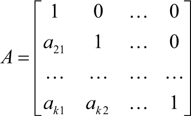
where Y_t denotes a k × 1 vector of variables with a lag length of ‘s’, A is the matrix of contemporaneous coefficients while F₁, F₂, …, F_s are the matrices of coefficients, u_t is assumed to have a mean 0 and fixed variance– covariance matrix Σ. The structure of matrix A is

A = [\begin{matrix} 1 & 0 & \dots & 0 \\ a_{21} & 1 & \dots & 0 \\ \dots & \dots & \dots & \dots \\ a_{k 1} & a_{k 2} & \dots & 1 \end{matrix}]

In other words, the equation could be rewritten as

y_{i ​, t} = {x^{'}}_{i ​, t} β_{t} + u_{i ​, t} i = 1, \dots, n t = 1, \dots, T

(2)

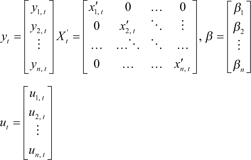
where y_{i, t} denotes the observation on the variable i at time t, x_{i, t} is a k-vector of lagged dependent explanatory variables. Considering all the endogenous variables jointly, Equation (2) looks like

y_{t} = X_{t}^{'} β + u_{t}

(3)

where y_t = [y_1t y2t, … y_nt] ´ is the n-vector of endogenous variables,

y_{t} = [\begin{matrix} y_{1, t} \\ y_{2, t} \\ ⋮ \\ y_{n, t} \end{matrix}] X_{t}^{'} = [\begin{matrix} x^{'}_{1, t} & 0 & \dots & 0 \\ 0 & x^{'}_{2, t} & ⋱ & ⋮ \\ \dots & \dots ⋱ & ⋱ & \dots \\ 0 & \dots & \dots & x^{'}_{n, t} \end{matrix}], β = [\begin{matrix} β_{1} \\ β_{2} \\ ⋮ \\ β_{n} \end{matrix}] u_{t} = [\begin{matrix} u_{1, t} \\ u_{2, t} \\ ⋮ \\ u_{n, t} \end{matrix}]

Now, considering a model with time-varying parameters and no restriction on the AR lag structure, Equation (2) can be written as

y_{i, t} = {x^{'}}_{i ​, t} β_{i ​, t} + u_{i ​, t} i = 1, \dots, n t = 1 \dots, T

(4)

Here y_{i, t} denote the observation of variable i at time t. Let x_{i, t} be a k_i x1 vector of explanatory variables for Equation (4). Now considering all the y_{i, t}’s jointly, Equation (3) looks like

y_{t} = X'_{t} β_{t} + u_{t}

(5)

Here y_{i, t} denote the observation of variable i at time t. Let x_{i, t} be a k_i x1 vector of explanatory variables for Equation (3). Now considering all the y_{i, t}’s jointly, Equation (3) looks like

y_{t} = [\begin{matrix} y_{1 ​, t} \\ y_{2 ​, t} \\ ⋮ \\ y_{n ​, t} \end{matrix}] X^{'}_{t} = [\begin{matrix} x^{'}_{1 ​, t} & 0_{1 x k_{2}} & \dots & 0_{1 x k_{n}} \\ 0_{1 x k_{1}} & x^{'}_{2 ​, t} & ⋱ & ⋮ \\ \dots & ⋱ & ⋱ & 0_{1 x k_{n}} \\ 0_{1 x k_{1}} & \dots & \dots & x^{'}_{n ​, t} \end{matrix}] β_{t} = [\begin{matrix} β_{1 ​, t} \\ β_{2 ​, t} \\ ⋮ \\ β_{n ​, t} \end{matrix}], u_{t} = [\begin{matrix} u_{1 ​, t} \\ u_{2 ​, t} \\ ⋮ \\ u_{n ​, t} \end{matrix}]

The vector of innovations u_t is assumed to have a multivariate normal distribution with mean zero and a covariance Ω_t that is, u_t ~ (0, Ω_t). This matrix can be decomposed using a triangular factorization that is, A_t Ω_t A'_t = Σ_t Σ'_t where A_t and Σ_t are n × n matrices having the following structure:

A = [\begin{matrix} 1 & 0 & \dots & 0 \\ a_{21 ​, t} & 1 & ⋱ & ⋮ \\ ⋱ & ⋮ & ⋱ & 0 \\ a_{k 1} & a_{k 2} & \dots & 1 \end{matrix}], \sum_{t} = [\begin{matrix} σ_{1 ​, t} & 0 & \dots & 0 \\ 0 & σ_{2 ​, t} & ⋱ & 0 \\ 0 & ⋱ & ⋱ & ⋱ \\ 0 & \dots & 0 & σ_{n, t} \end{matrix}]

Assuming u_t = A^–¹_t Σ_t ε_t, where ε_t is a n × 1 vector whose components have independent univariate normal distribution. Thus, Equation (5) can be rewritten as

y_{t} = {X^{'}}_{t} β_{t} + A_{t}^{- 1} \sum_{t} ε_{t} ε_{t} ~ (0, I_{n})

(6)

Thus,

y_{t} = c_{t} + B_{1 ​, t y t - 1} + \cdot \cdot \cdot + B_{k ​, t y t - k} + u_{t}

The elements of vector β_t are modelled as random walks. The standard deviations are assumed as geometric random walks, belonging to the class of models called stochastic volatility. All the innovations in the model are assumed to be jointly distributed and uncorrelated. The prior distribution of the variance–covariance matrix is assumed to follow inverse-Wishart. The prior distribution of the initial states of time-varying coefficients is assumed to be normally distributed. This is estimated using Gibbs sampling in the Markov Chain Monte Carlo algorithm.

The study focuses on the usage of the time-varying-impulse response function (IRF) following the methodology of Nakajima (2011) to analyse the impact of variables, namely, inflation, real GDP growth, and interest rate. For inflation, we use WPI and CPIIW to get the measures of both wholesale and retail inflation.

Results

First, we present the model with WPI as the wholesale inflation measure. We first analyse the stochastic volatility plots. The stochastic volatility helps in understanding the significant fluctuations in the macroeconomic time series under study. Next, we analyse the IRFs. Here, we estimate the IRFs by fixing the initial shock as the average of stochastic volatility measure for each variable and using the simultaneous relations at each point. We use the estimated time-varying coefficients to compute the IRFs from the current to future periods. We compare the time-varying IRFs with constant IRFs to have a better understanding of the result. We present the stochastic volatility plot in Figure 1.

Figure 1.

Stochastic Volatility Plot.

From the SV plot, we see that the WPI and GDP exhibited higher volatility during the COVID-19 crisis, whereas the interest rate was volatile during the subprime crisis of 2007–2008. Next, we analyse the constant IRFs. We provide unit shocks as three points in time. First, in 2018–2019 Q4 (before-COVID-19), then in 2020–2021 Q1 (COVID-19 period) and finally in 2021–2022 Q3 (Recovery period). We present the results in Figure 2.

Figure 2.

Estimated Constant IRFs at Three Periods.

From the IRF plot, we observe that the shape of the IRF is the same. However, the magnitude changes in certain cases. A shock from WPI initially results in a negative reaction of GDP, followed by an oscillatory pattern. A shock from WPI results in the increase of interest rate initially, followed by a drop after roughly 4 quarters or a year. However, the magnitude of the increase in the interest rates is lower in the COVID and the post-COVID period, as expected. A shock in GDP will lead to an initial increase in WPI, followed by a fall. In the COVID period, we see the magnitude of the fall is severe. A unit shock in GDP leads to an initial increase, followed by a decrease in the interest rate. The unit shock in interest rate leads to an initial increase in the WPI inflation, followed by a decrease. The unit shock in interest rate leads to an initial increase in GDP, followed by an oscillatory pattern. Next, we analyse the time-varying IRFs, presented in Figure 3. We estimate the time-varying IRFs with shocks ahead of 3, 6 and 12 quarters to capture the short, medium and long-run time-varying responses.

Figure 3.

Estimated Time-varying IRFs at 3, 6 and 12 Quarters.

From Figure 3, we see a shock in the WPI affected GDP growth positively in the short run. However, it hampers growth in the medium and long run (6 and 12 quarters ahead). We see that a shock in WPI leads to decreased interest rates in the aftermath of the 2007 and 2020 crises. This effect is visible in the short, medium and long run. A shock in GDP results in an increase in WPI across the short, medium and long run. However, the impact is more pronounced in the medium and long run during the COVID crisis whereas the short-run impact is more prevalent during the subprime crisis. A shock in GDP leads to a drop in the interest rate during the COVID crisis, across the short, medium and long run. A shock in the interest rate does not affect WPI in the short run. However, WPI is found to be decreasing both in the medium and long run. A shock in the interest rate is found to affect GDP in the short, medium and long run.

Next, we present the results for the retail inflation model. First, we present the stochastic volatility of all the variables, presented in Figure 4. From the plot, we find CPI-IW to be more volatile than WPI, which is to be expected. CPI-IW volatility is more pronounced in the subprime crisis period.

Figure 4.

Stochastic Volatility Plot.Next, we present the constant IRFs, estimated at three different points as mentioned above.

From the plot presented in Figure 5, we see that CPI-IW reacts differently from WPI, which was to be expected. A unit shock to CPI results in an initial drop in GDP, followed by an oscillatory response. We find this pattern to be more pronounced in the pre-COVID period. In the COVID and the recovery period, the amplitude of the oscillations is much subdued. A shock in CPI leads to a decrease in the interest rate. A shock in GDP leads to an initial increase in CPI, followed by an oscillatory response. We find that the amplitude of the initial increase in CPI is more pronounced in the COVID-19 and recovery periods. A shock in GDP leads to an initial increase in the interest rate, followed by a decline. The reaction is less pronounced in the recovery period. A shock in the interest rate initially increases the CPI, followed by a rapid decline. A shock in the interest rate initially results in an increase in GDP growth, followed by a sharp decline in an oscillatory fashion. Next, we analyse the time-varying IRF, presented in Figure 6.

Figure 5.

Estimated Constant IRFs at Three Periods.

Figure 6.

Estimated Time-varying IRFs at 3, 6 and 12 Quarters.

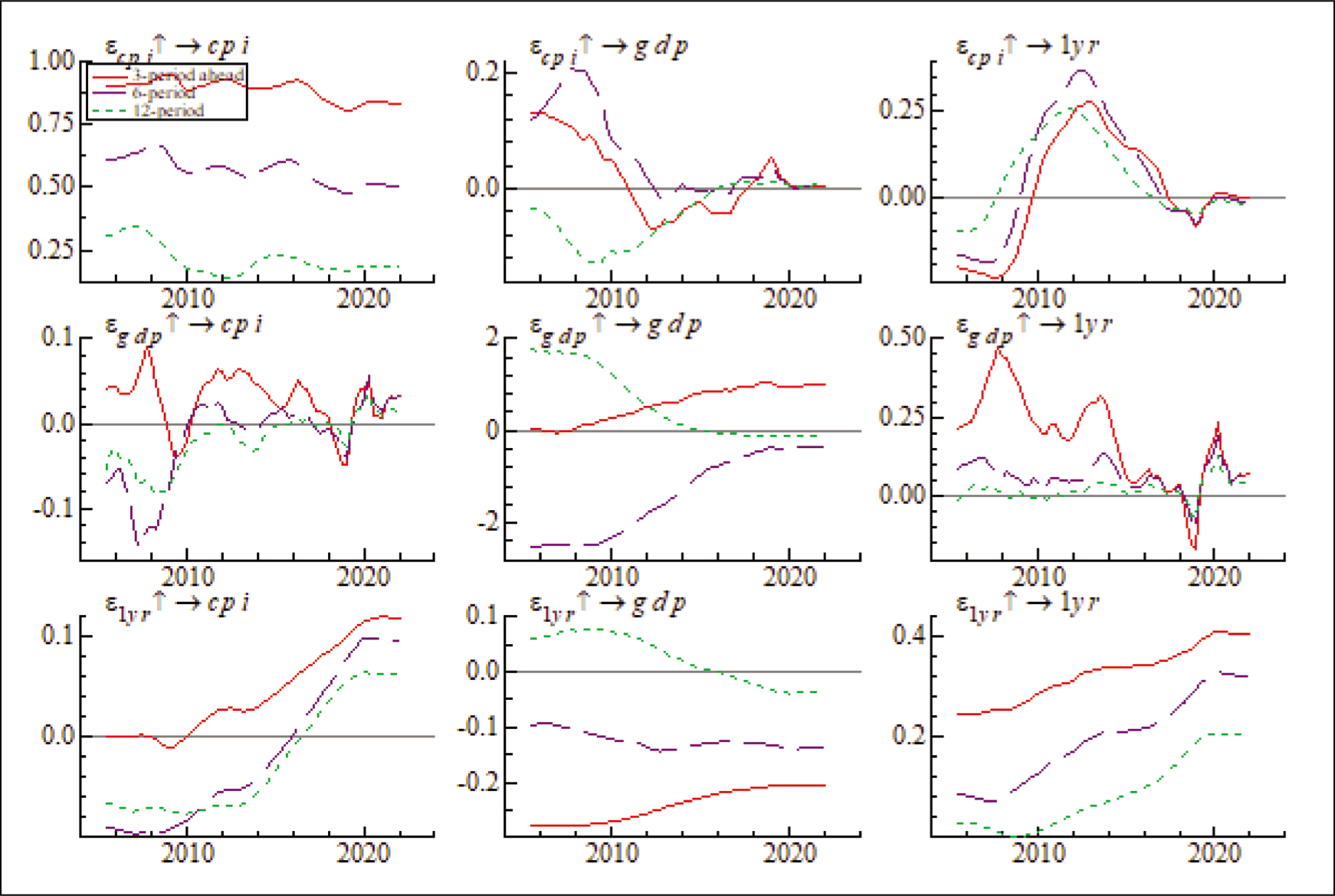
From the plot, we see that CPI-IW behaves radically different from the WPI, as postulated by the theory. A shock in CPI during the subprime crisis led to a significant drop in the GDP, both in the short and medium term. We find the same effect during COVID-19, but with a lesser magnitude. Similarly, a shock in CPI resulted in an increase in the interest rate after the subprime crisis for both the short, medium and long run. During COVID-19, a shock in CPI initially leads to a drop in the interest rate and later to an increase in the recovery period. A shock in GDP leads to a drop in CPI in the aftermath of the subprime crisis. This effect was more pronounced in the short and medium run. We observe the same during COVID-19 and here, the responses for both short, medium and long run are more or less synchronized. A shock in GDP leads to a drop in interest rates during both the subprime and the COVID-19 crisis. During the subprime crisis, we see that the three quarters ahead (short-run) reactions are more pronounced. During the COVID-19 period, all time-varying IRFs are synchronized. The response of CPI-IW to the interest rate shock is very different from that of WPI. During the subprime crisis, we see negligible response in the short, medium and long run. During the COVID-19 time, we see that a shock from the interest rate keeps the CPI-IW stable at best; we do not see any reduction in CPI across the short, medium and long run. The reaction of GDP growth to interest rate shock is rather flat during both the subprime crisis and COVID-19 in the short, medium and long run, pointing towards potential monetary policy ineffectiveness in stimulating the growth.

Conclusion and Policy Implication

Growth-inflation tradeoff has been the contentious ground of monetary policymaking. There are arguments for and against the monetary policy’s effectiveness in controlling inflation and supporting growth, both in the short term and long term. The central banking wisdom, however, has remained in favour of adapting to local conditions while evaluating sources of inflation and tempering policy response therewith. The COVID-19 pandemic has put this wisdom to test as central banks across the globe tighten monetary policy to curb inflation in near synchronized way. India is no exception with its inflation-targeting central bank caught in an unenviable position of defending credibility at a time when inflation stood outside its target band for ten consecutive months.

The supply shock brought by the pandemic has pronounced effect on India’s output and price situation. The source of price pressures has played differently in different measures of price dynamics, at the wholesale and retail level, thereby underscoring the sensitivity of nominal anchor in deciding interest rates as key to monetary policy effectiveness. Economic recovery post-pandemic has been a long drawn effort with monetary policy playing an enabler, though a weak one, in the presence of a large negative output gap. From our analysis, we find that a shock in the interest rate initially results in an increase in GDP growth, followed by a sharp decline in an oscillatory fashion. This further affirms weak correspondence of monetary policy for growth revival on a sustained basis. Recent data on output and inflation affirms this. While GDP is estimated to have grown at 7.2% in the financial year ended March 2023, inflation as measured by CPI averaged 6.7% during the period. Reflecting tightening monetary conditions, output has shown a decline with GDP growth estimated at 6.1% while inflation still averaged 6.2% in the fourth quarter of the financial year ended March 2023, thanks to easing fuel and food prices.

The monetary policy ineffectiveness pre- and post-pandemic could be attributed to different natures of supply shock, such as lockdown policy limiting economic activity in COVID affected areas, logistic delays in the availability of critical inputs like semi-conductors, fuel price spikes post the war in Europe broke out, etc. All this led to price build-up in early phases and then persistence thereon. The role of extraordinary demand stimulus, both fiscal and monetary, cannot be ignored either as it shifted the expectations of agents about money supply. In an environment full of uncertainty on the causes and nature of inflation, policymakers have been hesitant to respond effectively, especially in unwinding the demand-side stimulus, which partly explains inflation persistence at high levels (Rangarajan et al., 2023). Another view, though not much explored empirically, is about financial development reducing monetary policy effectiveness in emerging market economies with a rise in the share of non-bank institutions diminishing monetary transmission through credit channels (Ma & Lin, 2016). For India, more than elsewhere, investments matter to raise the production potential of the economy, which in turn could help with prices soothing down in the long term. Private sector share in investments has come down of late, as corporates with stressed financials went about deleveraging the balance sheet (Sahoo & Bishnoi, 2022). Encouragingly, the Government has stepped up to lead the capital expenditure cycle with Budgetary allocation for infrastructure reaching 3.3% of GDP for the financial year beginning 1 April 2023; the CapEx outlay in Budget 2023–2024 is almost three times to its pre-pandemic level in 2019–2020 (Government of India, 2022). However, as India’s public debt has increased to a historical high in the wake of the pandemic, better targeting of public debt is needed to improve growth without fuelling inflation, going forward (Singh & Kumar, 2022). Nuances matter in public policy. In our view, it would be erroneous for Indian monetary policymakers to go for interest rate overkill to keep inflationary expectations anchored like advanced economy central banks where citizens have better safety nets to overcome output sacrifices.

The RBI has maintained that monetary conditions remain accommodative as real interest rates have not been positive for much of the past year, and therefore, the MPC has persisted with ‘withdrawal of accommodation’ stance in the financial year 2023–2024 (Reserve Bank of India, 2023). Amid financial stability concerns in Advanced Economies, especially the USA with a string of bank failures making policymakers reminisce subprime crisis of 2008, thereby slowing the pace of monetary tightening, it is indeed welcome that MPC has opted to pause on interest rate hikes as the effect of cumulative 250 bps hike in policy rate work its way through economy.

From the aforesaid analysis, we draw two conclusions having policy implications. One, the RBI should avoid aggressive monetary policy tightening to curb inflation in the current cycle in sync with advanced economies. Varying sources of price impulses have played differently over time; especially in supply shocks like the pandemic, the CPI response to interest rate are found weak. Two, interest rates have little contribution to the revival of demand during pandemic, underscoring the need for fiscal measures doing heavy lifting on growth. Thus, the Government should continue with expansionary fiscal policy as monetary policy helps to keep financing costs low and inflation expectations anchored.

Footnotes

Declaration of Conflicting Interests

The authors declared no potential conflicts of interest with respect to the research, authorship and/or publication of this article.

Funding

The authors received no financial support for the research, authorship and/or publication of this article.

Notes

References

Anand

, Kumar

, & Tulin

M. V.

(2016). Understanding India’s food inflation: The role of demand and supply factors (Working Paper No. 2016/002). International Monetary Fund.

Badinger

(2008). Globalization, the output-inflation tradeoff, and inflation (FIW Working Paper No. 10).

Balakrishnan

, & Parameswaran

(2022). What lowered inflation in India: Monetary policy or commodity prices? Indian Economic Review, 57(1), 97–111.

Balcilar

, Ozdemir

, Aygun

, & Wohar

(2021). Effectiveness of monetary policy under the high and low economic uncertainty states: Evidence from the major Asian economies. Empirical Economics, 63, 1741–1769. 10.1007/s00181-021-02198-x

Ball

, & Mazumder

(2019). A Phillips curve with anchored expectations and short-term unemployment. Journal of Money, Credit and Banking, 51(1), 111–137.

Balleer

, & Noeller

(2023). Monetary policy in the presence of supply constraints: Evidence from German firm-level data (CESifo Working Paper No. 10261). https://dx-doi-org-s.web.bisu.edu.cn/10.2139/ssrn.4357553

Bhoi

B. K.

, Mitra

A. K.

, Singh

J. B.

, & Sivaramakrishnan

(2017). Effectiveness of alternative channels of monetary policy transmission: Some evidence for India. Macroeconomics and Finance in Emerging Market Economies, 10(1), 19–38.

Blanchard

, Cerutti

, & Summers

(2015). Inflation and activity–two explorations and their monetary policy implications (No. w21726). National Bureau of Economic Research.

Borio

, Hofmann

, & Zakrajšek

(2023). Does money growth help explain the recent inflation surge? (No. 67). Bank for International Settlements.

10.

Carstens

(5 April, 2022). The return of inflation. Speech at the International Center for Monetary and Banking Studies, Geneva.

11.

Cesa-Bianchi

, Thwaites

, & Vicondoa

(2020). Monetary policy transmission in the United Kingdom: A high frequency identification approach. European Economic Review, 123(C), S0014292120300076.

12.

Cogley

, & Sargent

T. J.

(2005). Drifts and volatilities: Monetary policies and outcomes in the post WWII US. Review of Economic Dynamics, 8(2), 262–302.

13.

Dasgupta

, & Chowdhury

(2023). Monetary policy in the midst of cost-push inflation. Economic & Political Weekly, 58(22), 42–50.

14.

Deheri

(2021). The effects of monetary policy on output and inflation in India: A time-varying approach. Economics Bulletin, 41(3), 1603–1614.

15.

Dua

(2020). Monetary policy framework in India. Indian Economic Review, 55(1), 117–154.

16.

Dua

, & Goel

(2021). Inflation persistence in India. Journal of Quantitative Economics, 19, 525–553. 10.1007/s40953-021-00237-z

17.

Dholakia

R. H.

(1990). Extended Phillips curve for the Indian economy. The Indian Economic Journal, 38(1), 69–78.

18.

Finck

(2019). Has monetary policy really become less effective in the euro area? A note. Applied Economics Letters, 26(13), 1087–1091.

19.

Forbes

(2019). Has globalization changed the inflation process? (Working Paper No. 791). Bank for International Settlements. https://www.bis.org/publ/work791.htm

20.

Fornaro

, & Wolf

(2023). The scars of supply shocks: Implications for monetary policy. Journal of Monetary Economics, 140, S18–S36.

21.

Goyal

, & Parab

P. M.

(2021). Effectiveness of expectations channel of monetary policy transmission: Evidence from India. Indira Gandhi Institute of Development Research.

22.

Government of India (2022). Budget documents for 2023. https://www.indiabudget.gov.in/

23.

Havranek

, & Rusnak

(2012). Transmission lags of monetary policy: A meta-analysis (Working Paper No. 1038). William Davidson Institute.

24.

Hazell

, Herreno

, Nakamura

, & Steinsson

(2022). The slope of the Phillips Curve: Evidence from US states. The Quarterly Journal of Economics, 137(3), 1299–1344.

25.

Irandoust

(2020). The effectiveness of monetary policy and output fluctuations: An asymmetric analysis. Australian Economic Papers, 59(2), 161–181.

26.

Junankar

P. N.

, & Wong

C. Y.

(2020). The impact of inflation targeting on inflation and growth: How Robust is the evidence? (IZA Discussion Paper No. 13284).

27.

Kapur

, & Patra

M. D.

(2000). The price of low inflation. Reserve Bank of India Occasional Papers, 21(2), 191–233.

28.

Kodjovi

M. E.

(2023). The anatomy of monetary policy transmission in an emerging market (IMF Working Papers 2023/146). International Monetary Fund.

29.

Lucas Jr

R. E.

(1976, January). Econometric policy evaluation: A critique. In Carnegie-Rochester conference series on public policy (Vol. 1, pp. 19)–46). North-Holland.

30.

, & Lin

(2016). Financial development and the effectiveness of monetary policy. Journal of Banking & Finance, 68, 1–11.

31.

Mishra

, Montiel

, & Sengupta

(2016). Monetary transmission in developing countries: Evidence from India (pp. 59–110). Springer India.

32.

Mohan

(2008). The role of fiscal and monetary policies in sustaining growth with stability in India. Asian Economic Policy Review, 3(2), 209–236.

33.

Nain

, & Kamaiah

(2020). Uncertainty and effectiveness of monetary policy: A Bayesian Markov Switching-VAR Analysis. Journal of Central Banking Theory and Practice, 9, 237–265. 10.2478/jcbtp-2020-0030

34.

Nakajima

(2011). Time-varying parameter VAR model with stochastic volatility: An overview of methodology and empirical applications. Monetary and Economic Studies, 29, 107–142

35.

Patnaik

, Shah

, & Bhattacharya

(2011). Monetary policy transmission in an emerging market setting. International Monetary Fund.

36.

Patra

M. D.

, & Ray

(2010). Inflation expectations and monetary policy in India: An empirical exploration. International Monetary Fund.

37.

Paul

B. P.

(2009). In search of the Phillips curve for India. Journal of Asian Economics, 20(4), 479–488.

38.

Rangarajan

(1983). Conflict between employment and inflation: Theory and facts. In Employment policy in a developing country a case-study of India Volume 1: Proceedings of a joint conference of the International Economic Association and the Indian Economic Association held in Pune, India (pp. 114–135). Palgrave Macmillan.

39.

Rangarajan

, Nachane

, & Ray

(2023). Monetary growth, financial structure, and inflation. Economic & Political Weekly, 58(22), 23.

40.

Reserve Bank of India (21 January 2014). Report of the expert committee to revise and strengthen the monetary policy framework (Patel Committee Report).

41.

Reserve Bank of India (2023). Governor’s Statement, RBI Bulletin, August 2023, Vol. LXXVII No. 8

42.

Sahoo

, & Bishnoi

(2023). Drivers of corporate investment in India: The role of firm-specific factors and macroeconomic policy. Economic Modelling, 125, 106330.

43.

Samuelson

P. A.

, & Solow

R. M.

(1960). Analytical aspects of anti-inflation policy. The American Economic Review, 50(2), 177–194.

44.

Singh

B. P.

, & Kumar

(2022). Public debt and economic growth in India: The new Evidence. Millennial Asia, 0(0). 10.1177/09763996221136908

45.

Sims

C. A.

, & Zha

(1999). Error bands for impulse responses. Econometrica, 67(5), 1113–1155.