The Information Content of Alternate Implied Volatility Models: Case of Indian Markets

Abstract

The information content to forecast the future realised volatility by model-based implied volatility and model free implied volatility has been an increasingly important area of research. There is a lot of literature suggesting that Black Scholes implied volatility is an efficient estimator (Fleming 1998); on the contrary there are studies suggesting that model free measures like VIX could be more informative (Jiang and Tian 2005). There is also a view, as evidenced in the earlier research, that there is a complete lack of relationship between them. The current study seeks to understand these dynamics in the Indian context and add to the debate by specifying market direction variables which could explain the relationship. The study tries to bring out the short-term relationship between the two volatilities. The present study finds evidence supporting Fleming (1998) and contrary to the evidence suggested by Jiang and Tian (2005), that is, Black Scholes implied volatility dominates the forecasting efficiency over the VIX even though both estimates are biased.

JEL Classification: G12, G13, G14, C22

Keywords

Black Scholes implied volatility VIX realised volatility historical volatility market efficiency generalised method of movements

Introduction

Volatility forecasting is a highly essential input for both risk management purposes and options trading. Many financial institutions need to maintain capital commensurate with their risky assets; volatility measures help them determine the capital adequacy. Similarly every option trader invariably requires the estimate of future volatility of the asset. In fact without the future volatility input, it is not possible to meaningfully give out quotes for trading in options market. Often the information in volatility has implication for option traders’ position payoffs. For instance, the implied volatility measure, that is, VIX fall could indicate overpricing in markets and could trigger correction.

A large body of literature is developed to capture the volatility process and it is believed that this area seems to be drawing increasing attention both by practitioners and academics (Poon 2005). On the one hand various statistical models depending on either constant volatility assumption or time varying assumptions propose alternate frameworks to capture the volatility process; on the other hand option pricing models and model free methods provide implied volatility measures to capture the process volatility. Many studies have linked both statistical and implied volatility models and tried to explain the information content of implied volatility to better understand the realised volatility (process volatility). Implied volatility is the expected future volatility based on market information. It should be an unbiased and efficient estimate of future process volatility given the condition that option markets are efficient. Some studies (Day and Lewis 1992; Lamoureux and Lastrappes 1993) which were carried out in the index and individual stocks context, report that implied volatility is both inefficient and biased estimate of realised volatility even though it has some predictive value. In yet another study (Canina and Figlewski 1993), an extreme result is reported suggesting that implied volatility has no relationship and has little information for realised volatility. Contrary to this, a few studies also reported that implied volatility outperforms many other forecasting methods like GARCH and is in fact efficient in forecasting realised volatility (Jorion 1995). According to Chirstensen and Prabhala (1998) and Fleming (1998), implied volatility is a biased estimator in the sense that it overestimates the realised volatility, yet is efficient. Many other studies follow the Fleming (1998) method and report similar results. These conflicting views provide evidence suggesting that implied volatilities either have information content or do not possess useful information for realised volatility.

The Indian derivatives market is about a decade old and much of the trading practices in derivatives are still developing. Many traders are still grappling with understanding the option pricing models and their implications for trading. In fact the relative trading of derivatives in India seem to be quite less compared to other in Asia of world over (Basu et al. 2006). While the market is gaining popularity both from Indian investing community and foreign investors, an understanding of the dynamics of price behaviour and its volatility in stock index markets needs to be researched. We intend to study whether alternate implied volatility measures have the information content for realised volatility in the Indian context. This is the primary motivation for our study.

Much of option trading is market direction based. Either traders trade a particular direction or against a particular direction. Especially model free implied volatility index is regarded as the fear index because when it falls one can anticipate a fall in the market. Do alternate implied volatility measures capture the information related to expected direction of the market? The previous studies have not explicitly analysed the information content of these variables in implied volatility. We propose two kinds of variables: One set of variables try to capture the monthly direction of the market and the other variable captures the daily direction of the market and attempts to see whether this information is subsumed by the alternative implied volatility measure. This is the second motive for the study.

The article attempts to develop an understanding of the dynamics of information content of alternate implied volatilities models, that is, Black Scholes implied volatility (hereafter BSIMC or BSIMP) and National Stock Exchange’s (NSE) VIX (hereafter NVIX) in the Indian stock index markets. Given the trading pattern in options market in India, where most of the trading is done in the near month option, an understanding of the information content of alternate implied volatility on realised volatility would be valuable, especially in the short term, that is, daily horizon.

The present study reports mixed results which indicate that the implied volatility measures (BSIMC/BSIMP and NVIX) are biased. However, the model-based implied volatilities (BSIMC/BSIMP) are efficient and subsume the information contained in model free implied volatility (NVIX) and option volumes in addition to a few other variables. These results are contrary to the findings reported by Jiang and Tian (2005) and are in support of Fleming (1998) and Becker et al. (2006).

In the following sections, initially we present an overview of Indian options market and then we discuss briefly the alternate empirical arguments by positing some select studies on the subject. This is followed by the methodological specification and nature of the data sets. The final part presents the results and conclusion of the study.

The Indian Derivatives Market

The Indian government banned forward trading over four decades ago with the view that it will avert speculative tendencies in the financial markets. This traditional view of the Government and the conservative financial policy was the reason for derivatives not being introduced in India. From 1991 onwards, with economic liberalisation, Indian economy witnessed a marked shift in the Government policy.

Securities and Exchange board of India (SEBI), which is the apex regulator of the financial markets, set up two committees successively, one headed by L.C. Gupta (1996) and the other by J.R. Varma (1998). The first committee highlighted the need for and the way derivative instruments could be introduced in India, which covered broad preconditions prior to introducing derivatives. Some of these preconditions were the need to recognise derivative instruments as securities for trading and the necessary change needed in the legislation. The J.R. Varma Committee worked out the modus operandi for derivative markets, by prescribing the regulatory provisions for traders and stock exchanges.

Derivative trading started in India in the year 2000. Even though SEBI permitted trading of derivatives in India’s biggest stock exchanges, that is, Bombay Stock Exchange (BSE) and the National Stock Exchange (NSE), trading is active only in NSE. NSE progressed by leaps and bounds ever since the trading in derivatives started and it is now awarded the Financial Derivatives Exchange of the year in 2010 by Asian Bankers Association. According to NSE in 2009 the average index linked futures contracts per day was close to 0.7 million and the average index options contracts was 1.3 millions.

NSE is the most modern stock exchange in India which runs on VSAT (Very Small Aperture Terminal) and is one of the largest VSAT-based stock exchanges in the world. It is based on a client server technology where traders are connected through computers seamlessly. These exchanges are popularly known as electronic contract networks in the literature and they differ from floor trading mechanism in a significant way. The information and price discovery in these markets are not determined by market makers and instead the exchange itself acts as the market maker.

Also the trading of derivatives markets and price discovery are related to the depth of derivatives market. As indicated earlier the relative trading of derivatives in India seem to be quite less compared to other derivative markets in Asia (Basu et al. 2006).

Some earlier studies found that Indian derivative markets are highly inefficient because it offers a lot of arbitrage opportunities (Vipul 2008). It is reported that derivative (futures) volatility and volume related information has a lot of persistence and leads the stock market volatility and volume which tantamount to market inefficiency.

Review of Literature

There is an abundance of literature in the area. We present select studies relevant for our discussion. The studies by Day and Lewis (1992) and Lamoureux and Lastrapes (1993) found evidence of little relationship between implied volatility and realised volatility. Also, Canina and Figlewski (1993) argued that the implied volatility is both biased and inefficient in forecasting the realised volatility.

However, Jorion (1995) found strong support about the predictive ability of implied volatility. His study used the implied standard deviations, which were calculated on CME options and their relative performance of forecasting the realised volatility was considered for the study. The findings suggest that the implied volatility measures are biased but perform much better than statistical measures of volatility like the EWMA and GARCH. Amin and Ng (1997) used HJM model to calculate the implied volatility in the Eurodollar market and found similar results where the implied volatility actually dominated both GARCH and Asymmetric GARCH measures. They question the methodology of Day and Lewis (1992) and also Lamoureux and Lastrapes (1993) method of including implied volatility as an exogenous variable in the GARCH specification and alter the specification to find evidence contrary to both the studies.

Chirstensen and Prabhala (1998) studied the predictive ability of Black Scholes implied volatility. They argued that much of Canina and Figlewshi (1993) results were the outcome of sampling errors. Their study came up with a sampling plan to reduce the overlap problem and considered other data problems that would reduce the errors in variables problem. Through a simple OLS methodology they found evidence against Canina and Figlewshi (1993) which indicates that implied volatilities are informative but are positively biased and could actually overpredict the realised volatility.

Fleming (1998) came up with a generalised method of movement (GMM) specification to study the predictive ability of Black Scholes implied volatility for both monthly and daily horizons. The findings support the study of Chirstensen and Prabhala (1998) but bring out the efficiency and information content debate. While the argument of estimate bias is founded, he attempted to answer whether these estimates are informationally inefficient. The GMM specification highlighted that the efficiency of the estimates cannot be rejected. Therefore implied volatility does contain information about the future volatility. His findings were much stronger in the daily data.

Becker et al. (2006) reported that implied volatilities are biased but are inefficient using the model free VIX as the measure for implied volatility. They have extensively calculated different measures of volatility and used the methodology suggested by Fleming (1998) and tested the hypothesis proposed by Harvey and Newbold (2000). Over 10 different measures of volatility were used in addition to four principal components of these volatilities in their model and found evidence that the implied volatilities’ ability to subsume a range of volatility information is inefficient. One other recent study by Jiang and Tian (2005) reports positive evidence in terms of predictive ability of model free implied volatilities. Their study constructs a model free measure based on Britten-Jones and Neuberger (2000) and tests the hypothesis whether the model free implied volatility subsumes the information of model-based implied volatility to forecast the realised volatility. Their evidence suggests that model free implied volatility measures clearly dominate inefficiency.

As can be seen from various arguments, the debate was initially about whether a relationship exists and whether this relationship is unbiased supporting the theoretical notion of efficiency in both options market and stock market. Much of the evidence now seems to support that the relationship is biased but implied volatilities do have information content. Then the question arises whether there is any alternate implied volatility specification that could well capture the realised volatility information. Quite a few studies report that model free implied volatilities dominate model-based implied volatility. But equally strong evidence supporting the case of model-based implied volatilities is found in the literature.

Methodology

Hypothesis and GMM Specification

From the perspective of forecasting, implied volatility should be an unbiased estimator of the realised volatility, because the market view of future volatility is impounded in the implied volatility. Therefore, implied volatility should subsume all information in predicting the future volatility. This is subject to the condition that the options markets are efficient in discounting all information available (Ω_t). Therefore, Equation (1) should hold.

σ_{t} = β_{t} I M_{t} + ε_{t} | Ω_{t},

(1)

where σ_t is the realised volatility of the population and IM_t is the implied volatility measure. If implied volatility is unbiased, β_t should equal one and value of the intercept not depicted above should be zero. The above argument holds if the options markets are completely linked to the stock markets and are efficient. Trading in both markets are active and traders can choose to trade the information either in the stock market or in the options markets. Both options market and the stock markets arrive at prices in a pooling equilibrium such that there are no arbitrage opportunities. Also for equation one to hold it is desirable that the model with which implied volatility is measured should be correct. If the model is biased then it would be a poor predictor of the realised volatility. Similarly, when there is sparse trading in either of the markets indicating that the markets are trying to find a separating equilibrium then the relationship could wane.

The sample specification of the above hypothesis is depicted in the following equations.

{\hat{σ}}_{t} = α_{t} + β_{t} B S I M C_{t} + u_{t}

(2)

{\hat{σ}}_{t} = α_{t} + β_{t} B S I M P_{t} + u_{t}

(3)

{\hat{σ}}_{t} = α_{t} + β_{t} N V I X_{t} + u_{t}

(4)

{\hat{σ}}_{t} = α_{t} + β_{t} {\hat{σ}}_{t - 1} + u_{t}

(5)

where ${\hat{σ}}_{t}$ is the log of realised volatility estimated on returns of 5-minute interval, BSIMC_t is the Log of Black Scholes call implied volatility, BSIMP_t is the Log of Black Scholes put implied volatility and NVIX_t is the log NSE implied volatility index. Equations (2) to (4) are elasticity models where all variables are expressed in log form. The Equation (5) is specified to test whether historical volatility contains the necessary information for realised volatility. The forecast error u_t should have all the properties of $ε_{t}$ and should be orthogonal to information set.

We used the generalised method of movements (GMM) on the dataset using the various volatility measures besides volumes and market direction variables as instrumental variables belonging to the information set Ω_t. As per the method proposed by Fleming (1998), we have tested whether the forecast errors of the specified models are orthogonal to known information variables. From our hypothesis as defined in the moment condition (2) through (5) the parameters α and β should be indistinguishable from zero and one, respectively, if implied volatilities are unbiased and or historical volatility is unbiased.

g (α, β) = \frac{1}{T} \sum_{t = 1}^{T} ({\hat{σ}}_{t} - α - β_{t} B S I M_{t}) z_{t},

(6)

where z_t are instrumental variables which include lags of BSIMC, BSIMP NVIX and historical volatility and instruments like MIBOR, PARK, CVOL, PVOL, BUY, MFLAT and MRISE. PARK is log transformed Parkinson (1980) range-based estimator, CVOL is log of call volume and PVOL is log of put volume. MFLAT is a dummy variable which takes the value of one when the market is flat for the month otherwise zero. MRISE is a dummy variable which takes the value of one when the market rises and otherwise it is zero. The variable BUY represents net option volumes. It takes the value of one if call option volume is greater than put option volume and zero otherwise. These variables are described in data section.

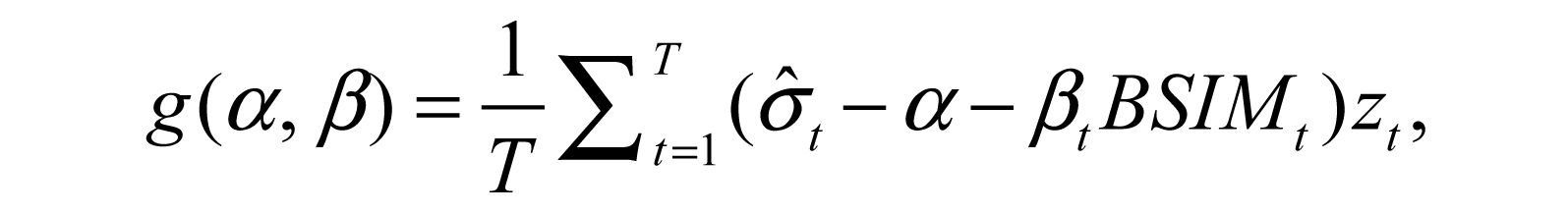
If the forecast errors demonstrate orthogonality then it can be said that the implied volatility subsumes the information contained in the information variable available at time t and therefore is informationally efficient. The parameter estimates g (α, β)′ according to the GMM framework are obtained as minimising the moment condition as stated in Equation (7).

J_{t} (α, β) = g (α, β)^{'} H_{t} g (α, β),

(7)

where H_t is the optimal covariance matrix that satisfies the minimisation criterion. However the system of moment condition will be overidentified with instrumental variables, since the system would have more equations with the instrumental variables than the parameters that need to be estimated. The GMM methodology allows for auto correlation and heteroscedasticity within the moment condition and finds the optimal matrix of weights that estimates the parameters as mentioned. The results would test the information content in the moment conditions and verify the parameter efficiency. The parameter efficiency is tested by the J-statistic. If the over identifying restrictions of the instruments are significant then the model parameters are inefficient and vice versa.

To test the unbiasedness of the parameters we imposed restrictions on α and β where α = 0 and β = 1. The Wald χ² is used to test the hypothesis in the moment conditions.

The Errors in Variables Problem

The primary concern of the empirical work in the literature was to deal with the errors in the variables problem. The problem arises because the independent variable is stochastic and therefore the errors are correlated with the covariates. Therefore, the coefficients are biased. The measurement error could be due to the model deficiencies or due to sampling. As far as the model deficiency is concerned our study uses the Black Scholes European (BS) option pricing model with dividend adjustment. Indian index options are European therefore many of the assumptions and model liberties taken in Fleming 1998 are not applicable to our study, while it may be true that the BS model itself may not be the preferred model for market participants. Even the model free method, that is, the VIX method of capturing the market volatility may not be the preferred method for market participants. The sampling related issues are discussed in the data section.

Data

Our datasets include stock index data and index options data of NSE. The study period is 1 January to 15 December 2006. Intraday data of the index and the options are extracted from the CDs provided by NSE on payment. The trading is active mostly in the near month options so we have taken contemporaneous index data and index options data. The index returns are initially calculated in 5-minute intervals and the standard deviation is calculated on the daily basis from the 5-min returns. We have made a correction to the standard deviation as suggested by Dacorogna et al. (2001) to remove the microstructure bias. There are 194 data points in the final data set.

Variable Definitions

The option implied volatility is calculated using the Black Scholes (1973) formula for both call and put options. Since index options in the Indian markets are European type, use of this formula is appropriate. We have made the dividend yield adjustment from the NSE index dividend data. We have calculated VIX as per the current method of NSE for the above mentioned period which represents the model free method of capturing market expected volatility. Our sample includes options from near, middle and far months; more than 90 per cent of sampled volatilities come from near month options because the most actively traded options are near month options. We have adopted the Jiang and Tian (2005) method of constructing the time series that is, we have chosen one single option series expiration at any given point in time and that which has at least eight days to expiry. This is consistent with NVIX calculation which is as per the NSE methodology. Every option series chosen for implied volatility calculation excludes the initial five days because most option experience rollovers and the effects of it could persist for at least five days. We have introduced three dummies to capture the market trends, i.e., MRISE, MFALL and MFLAT. MRISE takes the value of one if the market rises and other wise zero. Similarly MFLAT takes the value of one if the market is range bound otherwise it is zero. The market trend variables capture the market perception of price movements over a period of a month. Most option traders are either trading a particular market direction or hedging the against a possible market direction, volatility measures should contain the information of market direction.

The options pricing are determined by the trading activity and information of trading activity is depicted in volumes of options traded especially if call volumes (CVOL) pick up it may indicate that call prices could go up and vice versa if put volumes (PVOL) are traded in more number.

As per the argument put forward by Shanken (1990), the interest rates should predict the stock market volatility. We have used MIBOR which stands for Mumbai Inter Bank Offer Rate. This is a polled rate like LIBOR which we have used as a short-term measure of interest rate.

Similarly, many studies have related options volume to realised volatility (Sophie et al. 2008). We have taken the call option volumes and put options volumes which were traded in the last half hour near close and averaged them. We took the log of the option volumes and included them as instrumental variables in our analysis. We have also considered the net option volumes which would capture the direction of the market in a day as the explanatory variable. The variable BUY is a dummy variable which takes the value of one if the call option volumes for the day exceed put option volumes otherwise it takes the value of zero.

Besides we have used Parkinson’s (1980) range-based volatility (PARK) as an instrument which captures the daily extreme movement of prices. Implied volatility measures should contain the information of the extreme movements within a day.

Realised volatility is calculated as the standard deviation of the returns. Earlier studies (Chirstensen and Prabhala 1998; Jiang and Tian 2005 and many others) have used variance also as measure of realised volatility. It is also common to use the log of realised volatility in this literature. Andersen and Bollerslev (1998) point out the disadvantages of using daily data which could lead to inaccuracies. Accordingly there are advantages of using high frequency data. Also Andersen et al. (2001) point out the advantages of the log transformed realised volatility, since it is always positive and close to normal distribution. The returns were calculated in the five minute interval and the standard deviation of these historical returns is considered as the realised volatility. Since 5-min spaced volatility measure may have the bid/ask bounce we have corrected the volatility with a simple correction factor suggested by Dacorogna et al. (2001) which is given in Equation (8):

θ_{t} = \sqrt{\frac{Σ_{k = 1}^{z d} {[r_{5}]}^{2}}{Σ_{k = 1}^{z} {[r_{r e f}]}^{2}}}

(8)

where r₅ are returns measured in 5-min interval and r_ref is returns measured in a day or whatever is the reference period, it was one day for our study. The value z usually equals 260 and d is considered as equal to one day divided 5 mins intervals that would equal 288. The bias corrected standard deviation will be as in Equation (9).

σ_{b t} = \frac{σ_{t}}{θ_{t}},

(9)

where σ_bt is bias corrected 5-minute return volatility.

Implied Volatility models used in the study include both the Black Scholes Merton-based implied volatility and NSE’s VIX index. The method NSE uses is exactly the same as CBOE and is model free implied volatility measure. The variable BSIM is calculated for both call and puts (BSIMC and BSIMP) from the option traded in a day. We have averaged the last thirty minute implied volatilities which were calculated on traded at the money options as suggested by Harvey and Whaley (1992) and Fleming (1998). The moneyness of the option was determined by using the delta of the option. We choose option with the delta of about 0.5. We used near-month options (from 4 January to 15 December) for calculating Black Scholes implied volatility. However, we switched to middle month option series if the near-month option has eight (or less) days left to expiry. Similar method was followed by Jiang and Tian (2005). We used dividend yields and MIBOR rates from the NSE site for the whole period in the calculations. The option volumes were also calculated in the same manner as the implied volatilities. To avoid rollovers we have excluded 4 trading days after the expiry of near-month option.

NVIX index numbers for the year 2006 were not reported in the NSE site, so we have used the NSE method of calculation and calculated the NVIX for the period. We used Puts and Calls in two nearest month expiration (near and middle-month). However, if near-month option has eight (or less) days left to expiry, we switched to middle or far month options. The computations of volatilities for both the near and middle month were interpolated to obtain the volatility. Both BSIM and NVIX calculations were consistent.

As stated earlier we have considered the log transformed variable as suggested by Andersen et al. (2001) which is the quite prevalent in implied volatility and realised volatility studies. A list of the entire variables is being presented in Table 1.

Sampling of Time Series

Many studies reviewed by us among others have talked about the sampling of time series. It was observed that much of Canina and Figlewski (1993) results were due to wrong sampling. These sampling errors were highlighted to be telescoping overlap problems, which refers to the options expiration. Implied volatilities if calculated for a month will have overlapping time periods and as expiration approach the time decay could affect the volatility measures. All these studies tried to capture the relationship between implied volatility and realised volatility on monthly data. Since we are working on daily data much of these issues are not relevant for our study. However, telescoping could be an issue, with our data. We have resolved this problem by excluding the option series which has less than eight days to expiry. Also we worked on only near month option series and switched to middle month when the option had eight days to expiry.

Table 1.

List of Variables

Variable	Description
RV	Log of the volatility calculated on returns of 5 minutes
BSIMC	Log of Black Scholes implied volatility of call traded in the last 30 minutes near the close
BSIMP	Log of Black Scholes implied volatility of puts traded in the last 30 minutes near the close
BSIMC lag	First lag of BSIMC
BSIMP lag	First lag of BSIMP
RV lag	First lag of realised volatility, taken as the measure for historical volatility
NVIX	Log of the Model free volatility calculated daily as per the NSE methodology
NVIX lag	First lag of NVIX
MFLAT	Dummy variable takes the value of 1 if the market month is flat and 0 otherwise
MRISE	Dummy variable takes the value of 1 if the market month is rising and 0 otherwise
CVOL	Log of call volumes
PVOL	Log of put volumes
MIBOR	Daily MIBOR as reported by NSE FIMMDA
PARK	Log of Parkinnson 1980 volatility
BUY	Dummy variable takes the value of 1 if call volumes exceed put volumes and 0 otherwise

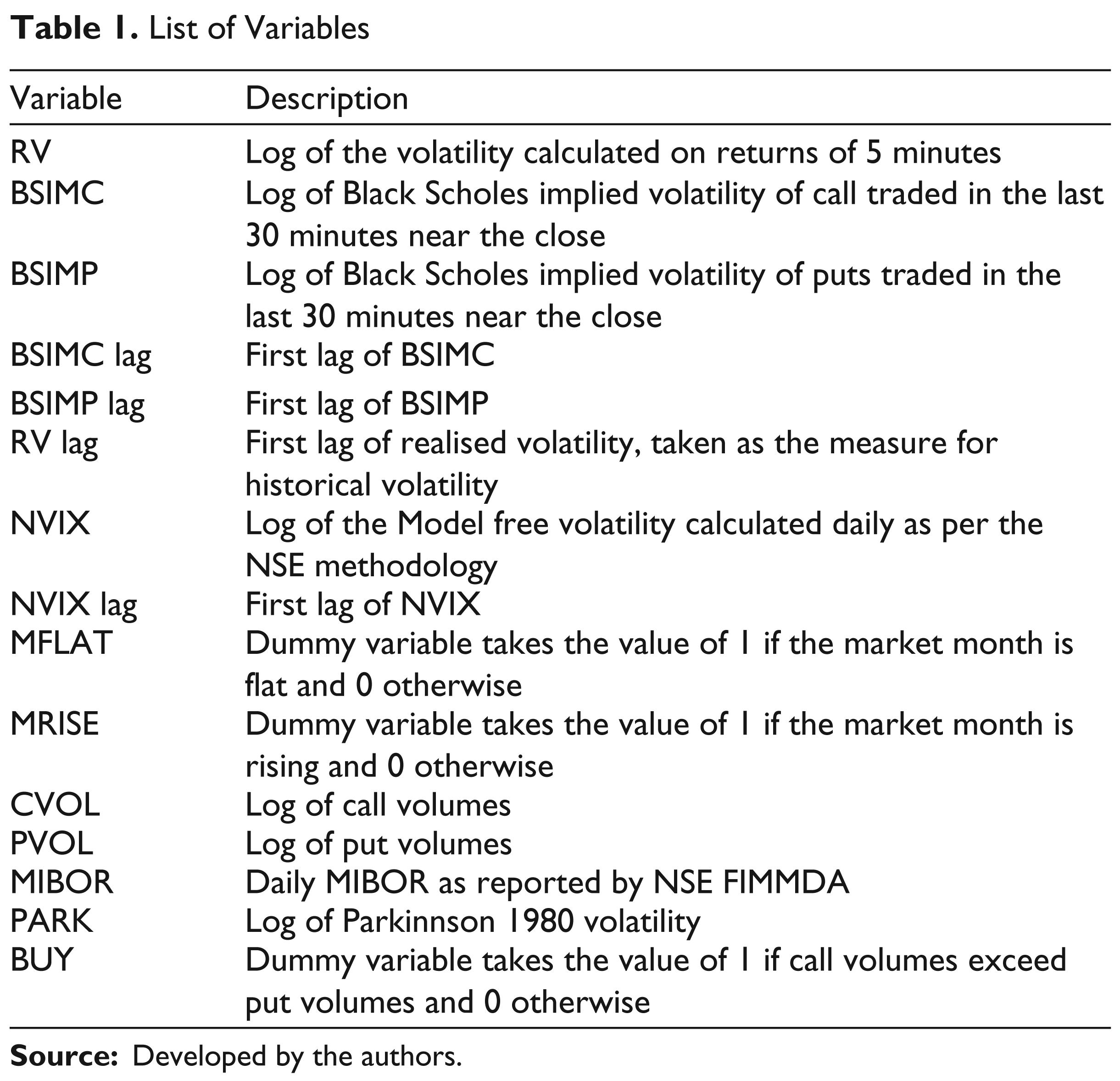
Source: Developed by the authors.

Descriptive Statistics and Correlations

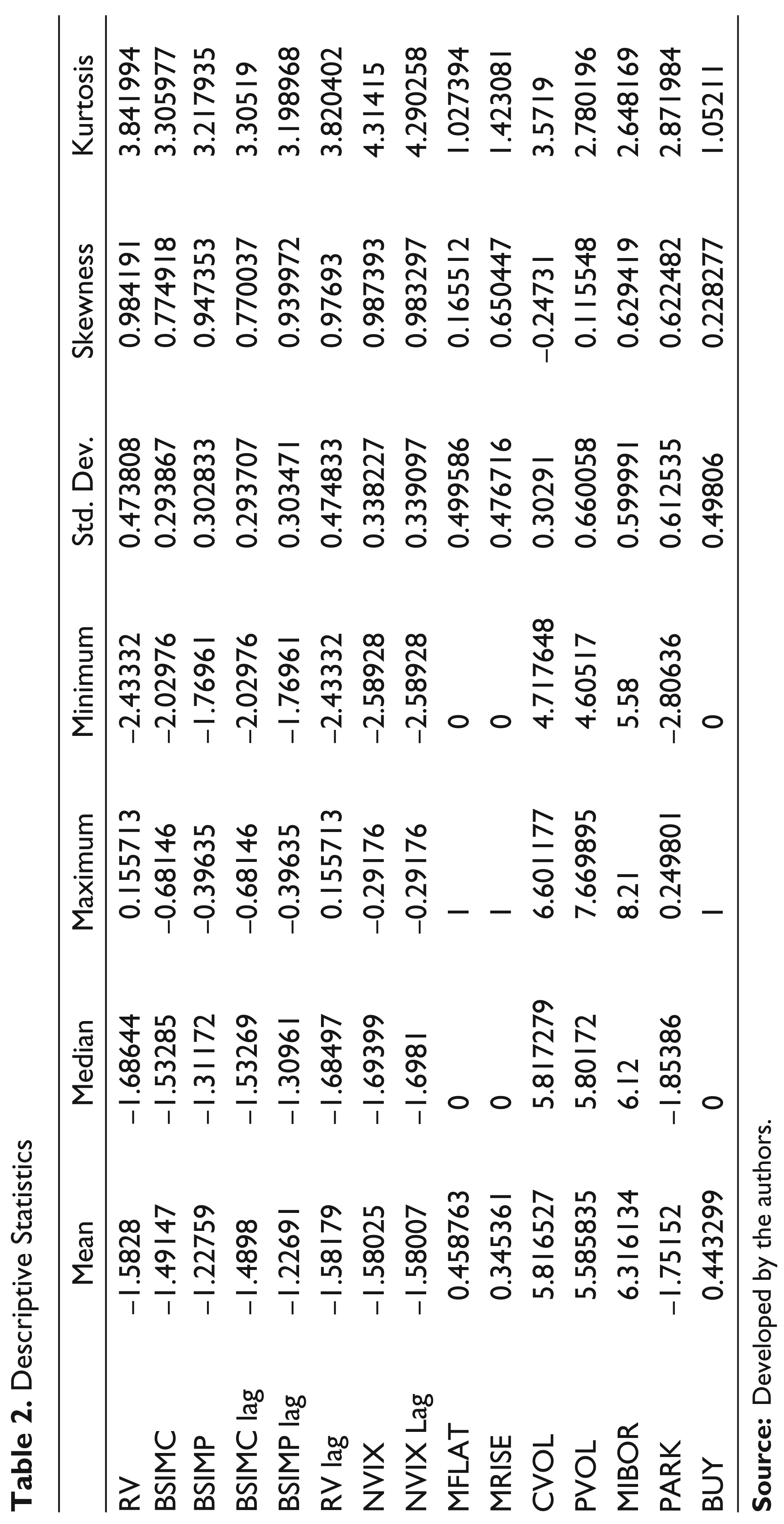
The descriptive statistics presented in Table 2 give a snap shot of the all the volatilities and the basic distributional properties. Most of the volatilities excepting seem to be in the range of 21 per cent to 23 per cent (not shown in the table). Most volatilities kurtosis is above three. There is a marked reduction in kurtosis. Since we considered the last half an hour option prices and averaged them, as suggested by Harvey and Whaley (1992), the implied volatilities kurtosis is reduced. Without averaging they had high kurtosis (not reported in the table).

Table 2.

Descriptive Statistics

	Mean	Median	Maximum	Minimum	Std. Dev.	Skewness	Kurtosis
RV	–1.5828	–1.68644	0.155713	–2.43332	0.473808	0.984191	3.841994
BSIMC	–1.49147	–1.53285	–0.68146	–2.02976	0.293867	0.774918	3.305977
BSIMP	–1.22759	–1.31172	–0.39635	–1.76961	0.302833	0.947353	3.217935
BSIMC lag	–1.4898	–1.53269	–0.68146	–2.02976	0.293707	0.770037	3.30519
BSIMP lag	–1.22691	–1.30961	–0.39635	–1.76961	0.303471	0.939972	3.198968
RV lag	–1.58179	–1.68497	0.155713	–2.43332	0.474833	0.97693	3.820402
NVIX	–1.58025	–1.69399	–0.29176	–2.58928	0.338227	0.987393	4.31415
NVIX Lag	–1.58007	–1.6981	–0.29176	–2.58928	0.339097	0.983297	4.290258
MFLAT	0.458763	0	1	0	0.499586	0.165512	1.027394
MRISE	0.345361	0	1	0	0.476716	0.650447	1.423081
CVOL	5.816527	5.817279	6.601177	4.717648	0.30291	–0.24731	3.5719
PVOL	5.585835	5.80172	7.669895	4.60517	0.660058	0.115548	2.780196
MIBOR	6.316134	6.12	8.21	5.58	0.599991	0.629419	2.648169
PARK	–1.75152	–1.85386	0.249801	–2.80636	0.612535	0.622482	2.871984
BUY	0.443299	0	1	0	0.49806	0.228277	1.05211

Source: Developed by the authors.

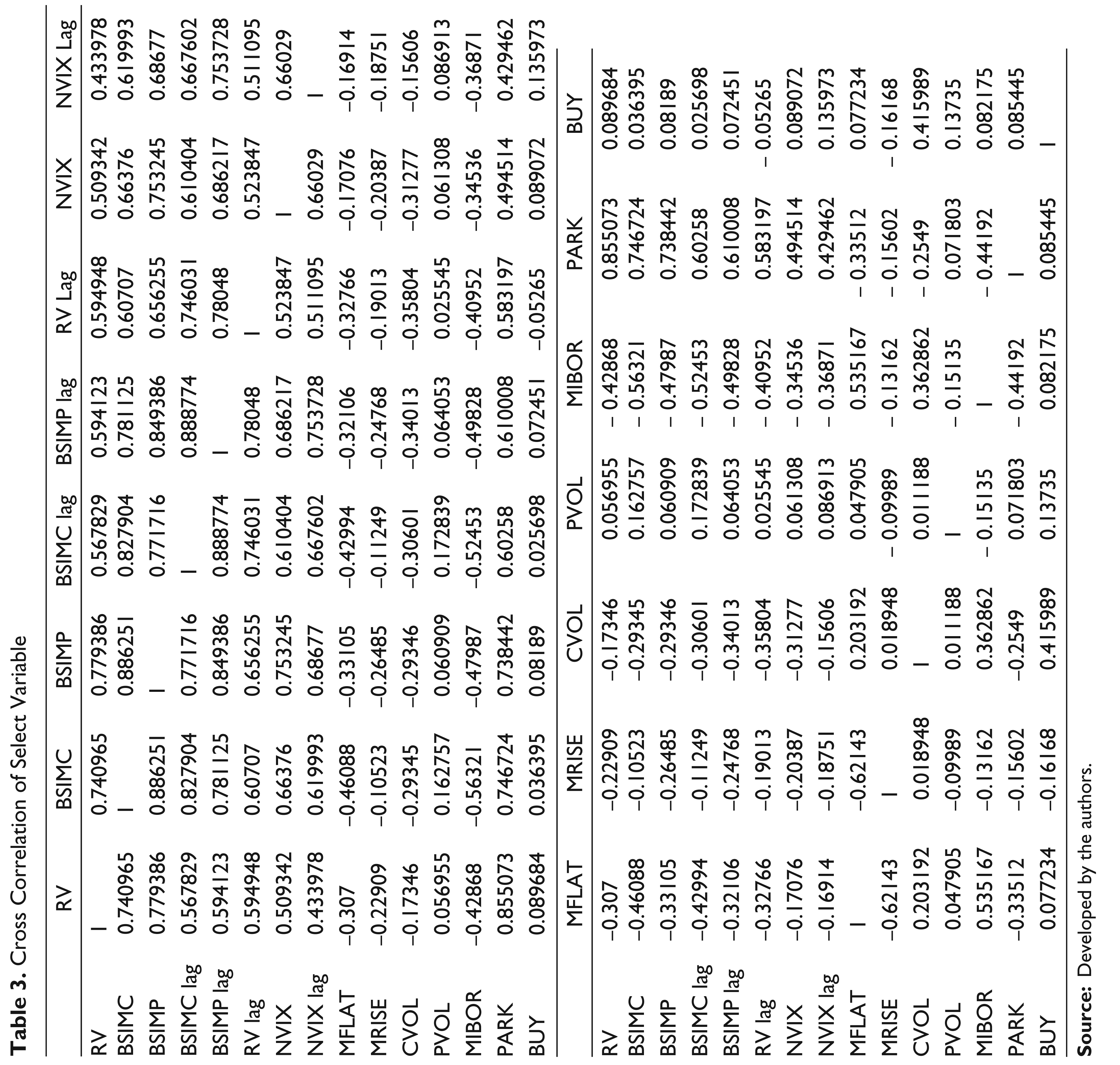
Cross correlations among variables are shown in Table 3. Realised volatility is highly correlated with BSIMC and BSIMP that is, 0.74 and 0.77, respectively. Its correlation reduces when it comes to NVIX, that is, 0.5. Its correlation is negative to MFLAT, MRISE and CVOL. Intuitively this is consistent with the volatility behaviour because when markets rise the volatilities usually fall and when markets fall the volatilities rise. Also the volatilities should be negatively correlated with call volumes because when call volumes rise the markets will rise and volatilities fall. The correlation of realised volatility is positive with PVOL, which is also consistent; when put volumes increase markets may fall therefore volatilities may rise. It is negatively related to MBOR and has little relationship with the variable BUY. When interest rates rise volatilities may fall because with interest rate rise call prices will go up but put price will come down, suggesting a consistent relationship. It has highest relationship with the range-based Parkinson (1980) volatility.

The model-based implied volatilities also show a similar and consistent relationship with other variables. BSIMC and BSIMP have a correlation of 0.88. BSIMC has 0.66 correlation with NVIX whereas BSIMP has 0.75 correlation with NVIX. The model-based volatilities have similar relationships with other variable as realised volatility above which is consistent to the hypothesised relationships discussed earlier.

The short-term interests MIBOR has 0.5 correlation with MFLAT and –0.13 with MRISE suggesting that markets may experience little price changes when the interest rates rise, while markets rise when interest rates fall. Its relationship with CVOL is positive and PVOL is negative which is consistent.

The short-term market direction as measured by BUY has very low correlation with almost all variables. It has the highest positive correlation with CVOL which is on the expected lines.

Table 3.

Cross Correlation of Select Variable

	RV	BSIMC	BSIMP	BSIMC lag	BSIMP lag	RV Lag	NVIX	NVIX Lag
RV	1	0.740965	0.779386	0.567829	0.594123	0.594948	0.509342	0.433978
BSIMC	0.740965	1	0.886251	0.827904	0.781125	0.60707	0.66376	0.619993
BSIMP	0.779386	0.886251	1	0.771716	0.849386	0.656255	0.753245	0.68677
BSIMC lag	0.567829	0.827904	0.771716	1	0.888774	0.746031	0.610404	0.667602
BSIMP lag	0.594123	0.781125	0.849386	0.888774	1	0.78048	0.686217	0.753728
RV lag	0.594948	0.60707	0.656255	0.746031	0.78048	1	0.523847	0.511095
NVIX	0.509342	0.66376	0.753245	0.610404	0.686217	0.523847	1	0.66029
NVIX lag	0.433978	0.619993	0.68677	0.667602	0.753728	0.511095	0.66029	1
MFLAT	–0.307	–0.46088	–0.33105	–0.42994	–0.32106	–0.32766	–0.17076	–0.16914
MRISE	–0.22909	–0.10523	–0.26485	–0.11249	–0.24768	–0.19013	–0.20387	–0.18751
CVOL	–0.17346	–0.29345	–0.29346	–0.30601	–0.34013	–0.35804	–0.31277	–0.15606
PVOL	0.056955	0.162757	0.060909	0.172839	0.064053	0.025545	0.061308	0.086913
MIBOR	–0.42868	–0.56321	–0.47987	–0.52453	–0.49828	–0.40952	–0.34536	–0.36871
PARK	0.855073	0.746724	0.738442	0.60258	0.610008	0.583197	0.494514	0.429462
BUY	0.089684	0.036395	0.08189	0.025698	0.072451	–0.05265	0.089072	0.135973

	MFLAT	MRISE	CVOL	PVOL	MIBOR	PARK	BUY
RV	–0.307	–0.22909	–0.17346	0.056955	– 0.42868	0.855073	0.089684
BSIMC	–0.46088	–0.10523	–0.29345	0.162757	– 0.56321	0.746724	0.036395
BSIMP	–0.33105	–0.26485	–0.29346	0.060909	– 0.47987	0.738442	0.08189
BSIMC lag	–0.42994	–0.11249	–0.30601	0.172839	– 0.52453	0.60258	0.025698
BSIMP lag	–0.32106	–0.24768	–0.34013	0.064053	– 0.49828	0.610008	0.072451
RV lag	–0.32766	–0.19013	–0.35804	0.025545	– 0.40952	0.583197	– 0.05265
NVIX	–0.17076	–0.20387	–0.31277	0.061308	– 0.34536	0.494514	0.089072
NVIX lag	–0.16914	–0.18751	–0.15606	0.086913	– 0.36871	0.429462	0.135973
MFLAT	1	–0.62143	0.203192	0.047905	0.535167	– 0.33512	0.077234
MRISE	–0.62143	1	0.018948	– 0.09989	– 0.13162	– 0.15602	– 0.16168
CVOL	0.203192	0.018948	1	0.011188	0.362862	– 0.2549	0.415989
PVOL	0.047905	–0.09989	0.011188	1	– 0.15135	0.071803	0.13735
MIBOR	0.535167	–0.13162	0.362862	– 0.15135	1	– 0.44192	0.082175
PARK	–0.33512	–0.15602	–0.2549	0.071803	– 0.44192	1	0.085445
BUY	0.077234	–0.16168	0.415989	0.13735	0.082175	0.085445	1

Source: Developed by the authors.

Results and Discussion

Information in Call Implied Volatility

The ‘Hypothesis and GMM Specification’ section of methodology above highlights the significant hypothesis of the present study. The hypothesis mentioned in Equations (1) and (2) says that BSIMC is an unbiased estimate of realised volatility. Also, we hypothesise that the information in the instrumental variables such as MRISE, MFLAT which are directional variables are subsumed in the implied volatility. Similarly, we extend the hypothesis to include other instruments such as CVOL, PVOL, BUY, MIBOR, NVIX and PARK, the information in all these variables are hypothesised to be subsumed by BSIMC.

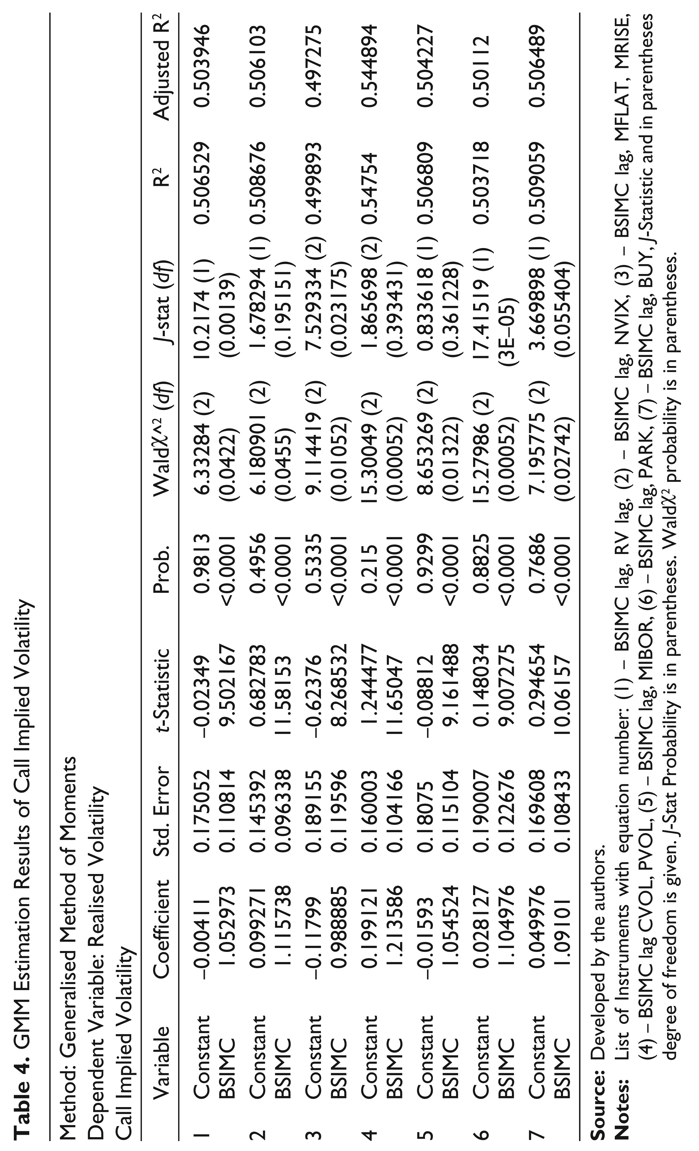
Table 4 presents the results of GMM regressions where the dependent variable is the log of realised volatility calculated on five minute returns and the independent variable is BSIMC, which is log of the Black Scholes call implied volatility. In all regression baring Equations (3) and (4) the results show that the coefficients of α and β as close to zero and one. The t-statistic probabilities suggest that α is insignificant and βas highly significant (< 0.0001 probability). But in all of these regressions the Wald χ^2 statistic rejects the hypothesis that α = 0 and β = 1. Therefore call implied volatility is a biased estimate of realised volatility. Further, the Equations (1) through (7) have used varying instruments from the information set at time t. The forecast error is hypothesised to be orthogonal to the information in the instrument set. Equation (1) rejects the hypothesis that the over identifying restrictions of the instruments, that is, lag of BSIMC and realised volatility lag are insignificant as depicted in the J-statistic. The call implied volatility does not contain the information of the historical volatility and therefore is inefficient. Similarly, BSIMC does not contain the information related to MFLAT and MRISE, which are directional variables and it does not subsume the information in PARK and BUY as depicted in Equations (3), (5) and (7), respectively. While call implied volatility does contain the information in the model free volatility, that is, NVIX as indicated by the results in Equation (2) by the J-statistic. All information at time t in NVIX is fully subsumed by BSIMC and therefore BSIMC is efficient informationally. Likewise BSIMC subsumes the information in CVOL and PVOL, also it fully subsumes information in MIBOR, the short-term interest rate.

Call implied volatility does have the information for future volatility but it is biased and does not contain information related to the historical volatility, range-based volatility and market direction variables. While it contains information related to volumes, interest rate and the information in model free volatility which are generally used as indicators for assessing future volatility. Perhaps Indian option traders seem to rely on Black Scholes pricing methodology the implied volatility as calculated through the Black Scholes method seem to convey information of all trading related variables like volumes. It seems to also contain information of interest rates which is one of the key inputs of the option pricing and also the model free implied volatility itself.

Table 4.

GMM Estimation Results of Call Implied Volatility

Method: Generalised Method of MomentsDependent Variable: Realised VolatilityCall Implied Volatility
	Variable	Coefficient	Std. Error	t-Statistic	Prob.	Waldχ^² (df)	J-stat (df)	R²	Adjusted R²
1	Constant	–0.00411	0.175052	–0.02349	0.9813	6.33284 (2)	10.2174 (1)	0.506529	0.503946
	BSIMC	1.052973	0.110814	9.502167	<0.0001	(0.0422)	(0.00139)
2	Constant	0.099271	0.145392	0.682783	0.4956	6.180901 (2)	1.678294 (1)	0.508676	0.506103
	BSIMC	1.115738	0.096338	11.58153	<0.0001	(0.0455)	(0.195151)
3	Constant	–0.11799	0.189155	–0.62376	0.5335	9.114419 (2)	7.529334 (2)	0.499893	0.497275
	BSIMC	0.988885	0.119596	8.268532	<0.0001	(0.01052)	(0.023175)
4	Constant	0.199121	0.160003	1.244477	0.215	15.30049 (2)	1.865698 (2)	0.54754	0.544894
	BSIMC	1.213586	0.104166	11.65047	<0.0001	(0.00052)	(0.393431)
5	Constant	–0.01593	0.18075	–0.08812	0.9299	8.653269 (2)	0.833618 (1)	0.506809	0.504227
	BSIMC	1.054524	0.115104	9.161488	<0.0001	(0.01322)	(0.361228)
6	Constant	0.028127	0.190007	0.148034	0.8825	15.27986 (2)	17.41519 (1)	0.503718	0.50112
	BSIMC	1.104976	0.122676	9.007275	<0.0001	(0.00052)	(3E–05)
7	Constant	0.049976	0.169608	0.294654	0.7686	7.195775 (2)	3.669898 (1)	0.509059	0.506489
	BSIMC	1.09101	0.108433	10.06157	<0.0001	(0.02742)	(0.055404)

Source: Developed by the authors.

Notes: List of Instruments with equation number: (1) – BSIMC lag, RV lag, (2) – BSIMC lag, NVIX, (3) – BSIMC lag, MFLAT, MRISE, (4) – BSIMC lag CVOL, PVOL, (5) – BSIMC lag, MIBOR, (6) – BSIMC lag, PARK, (7) – BSIMC lag, BUY, J-Statistic and in parentheses degree of freedom is given. J-Stat Probability is in parentheses. Waldχ² probability is in parentheses.

Put Implied Volatility

As per hypothesis in Equations (1) and (3), the Black Scholes put implied volatility is an unbiased estimate of the realised volatility. Also, it contains all the information in the instrumental variables like MRISE, MFLAT which are directional variables, CVOL, PVOL, BUY, MIBOR, NVIX and PARK.

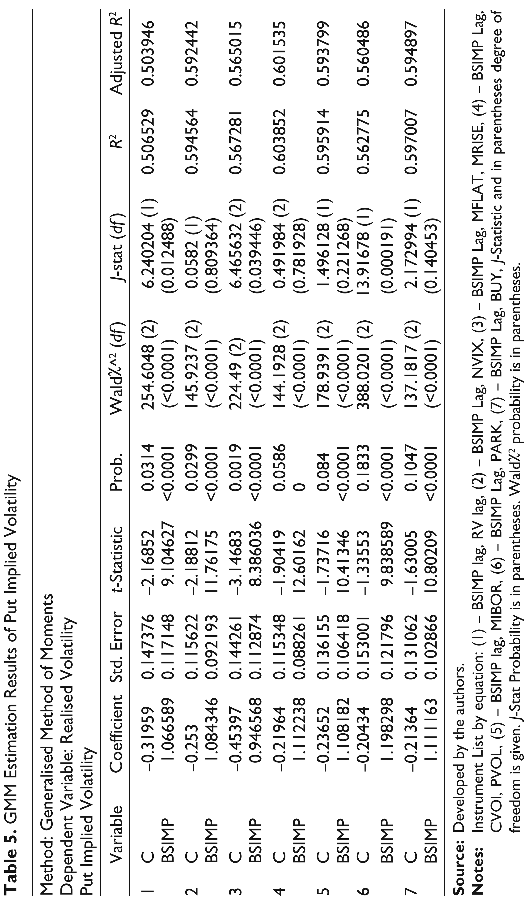
Table 5 presents the GMM regression results for put implied volatilities. The explanatory power of put implied volatility is greater than the call implied volatility. In all of the regressions, the t-statistic for the intercept is significant for both the intercept and BSIMP. The Wald χ^2 statistic rejects the hypothesis that α = 0 and β = 1. Therefore, put implied volatilities are biased and overstate the future volatility. The orthogonality test for Equations (1), (3) and (6) reject the hypothesis that the over identifying restrictions of instruments are not significant. Which suggest that put implied volatilities do not contain information related to historical volatility, directional variables MFLAT and MRISE and range-based estimate PARK. But Equations (2), (4), (5) and (7) support non-rejection of the hypothesis that the over identifying restriction of the instruments are not significant. Implying that the information in model free volatility NVIX, option volumes CVOL, PVOL, interest rates MIBOR and the directional variable BUY is subsumed by the put implied volatility.

Put implied volatility score over the call implied volatility because they seem to also contain information of the short-term direction of the future volatility. Put implied volatility subsumes information in model free volatility like the call implied volatility. The information in volumes and short-term interests is also contained in the put implied volatility. The results corroborate our earlier finding that perhaps Indian option traders use of Black Scholes pricing method.

Table 5.

GMM Estimation Results of Put Implied Volatility

Method: Generalised Method of MomentsDependent Variable: Realised VolatilityPut Implied Volatility
	Variable	Coefficient	Std. Error	t-Statistic	Prob.	Waldχ^² (df)	J-stat (df)	R²	Adjusted R²
1	C	–0.31959	0.147376	–2.16852	0.0314	254.6048 (2)	6.240204 (1)	0.506529	0.503946
	BSIMP	1.066589	0.117148	9.104627	<0.0001	(<0.0001)	(0.012488)
2	C	–0.253	0.115622	–2.18812	0.0299	145.9237 (2)	0.0582 (1)	0.594564	0.592442
	BSIMP	1.084346	0.092193	11.76175	<0.0001	(<0.0001)	(0.809364)
3	C	–0.45397	0.144261	–3.14683	0.0019	224.49 (2)	6.465632 (2)	0.567281	0.565015
	BSIMP	0.946568	0.112874	8.386036	<0.0001	(<0.0001)	(0.039446)
4	C	–0.21964	0.115348	–1.90419	0.0586	144.1928 (2)	0.491984 (2)	0.603852	0.601535
	BSIMP	1.112238	0.088261	12.60162	0	(<0.0001)	(0.781928)
5	C	–0.23652	0.136155	–1.73716	0.084	178.9391 (2)	1.496128 (1)	0.595914	0.593799
	BSIMP	1.108182	0.106418	10.41346	<0.0001	(<0.0001)	(0.221268)
6	C	–0.20434	0.153001	–1.33553	0.1833	388.0201 (2)	13.91678 (1)	0.562775	0.560486
	BSIMP	1.198298	0.121796	9.838589	<0.0001	(<0.0001)	(0.000191)
7	C	–0.21364	0.131062	–1.63005	0.1047	137.1817 (2)	2.172994 (1)	0.597007	0.594897
	BSIMP	1.111163	0.102866	10.80209	<0.0001	(<0.0001)	(0.140453)

Source: Developed by the authors.

Notes: Instrument List by equation: (1) – BSIMP lag, RV lag, (2) – BSIMP Lag, NVIX, (3) – BSIMP Lag, MFLAT, MRISE, (4) – BSIMP Lag, CVOl, PVOL, (5) – BSIMP lag, MIBOR, (6) – BSIMP Lag, PARK, (7) – BSIMP Lag, BUY, J-Statistic and in parentheses degree of freedom is given. J-Stat Probability is in parentheses. Waldχ² probability is in parentheses.

Model Free Implied Volatility

As per hypothesis in Equations (1) and (4), the model free implied volatility is an unbiased estimate of the realised volatility. Also it contains all the information in the instrumental variables like MRISE, MFLAT which are directional variables, CVOL, PVOL, BUY, MIBOR PARK and information present in model-based implied volatility (BSIMC and BSIMP).

The results for model free volatility as depicted in Table 6 point out that in all of the regression the t-statistic for the intercept and the independent variable NVIX are insignificant and significant, respectively. But the Wald χ^2 statistic rejects the hypothesis that α = 0 and β = 1 in all the regressions suggesting that NVIX is biased. Also the explanatory power, that is, adjusted R²is markedly reduced when compared to the results in Tables 4 and 5. The orthogonality tests (J-statistic) in Equations (1), (2), (3) and (7) reject the hypothesis that the over identifying restrictions of the instruments like historical volatility, call implied volatility, put implied volatility and range-based Parkinson volatility, are not significant. Whereas the Equations (5) and (8) clearly support the non rejection of the hypothesis that the overidentifying restrictions of instruments like option volumes and the market direction variable like BUY are not significant. The Equations (4) and (6) also support non-rejection of the hypothesis of orthogonality but are on the borderline.

Table 6.

GMM Estimation Results of Model Free Volatility

Method: Generalised Method of MomentsDependent Variable: Realised VolatilityModel Free Implied Volatility
	Variable	Coefficient	Std. Error	t-Statistic	Prob.	Waldχ^²(df)	J-stat (df)	R²	Adjusted R²
1	C	–0.05388	0.20216	–0.2665	0.7901	3.663397 (2)	3.707728 (1)	0.215613	0.211506
	NVIX	1.003104	0.120971	8.292102	<0.0001	(0.1601)	(0.054161)
2	C	–0.04281	0.20187	–0.21208	0.8323	4.036602 (2)	4.72972 (1)	0.210048	0.205912
	NVIX	1.013313	0.121112	8.366745	<0.0001	(0.1329)	(0.029646)
3	C	–0.0546	0.204461	–0.26703	0.7897	5.894681 (2)	4.529706 (1)	0.207696	0.203548
	NVIX	1.009641	0.122705	8.228208	<0.0001	(0.0525)	(0.033311)
4	C	–0.11123	0.211726	–0.52536	0.5999	5.605915 (2)	4.869206 (2)	0.217514	0.213417
	NVIX	0.973664	0.129934	7.493552	<0.0001	(0.0606)	(0.087633)
5	C	–0.16396	0.207849	–0.78885	0.4313	0.656464 (2)	0.208356 (2)	0.239552	0.235105
	NVIX	0.892784	0.132369	6.744677	<0.0001	(0.7202)	(0.901065)
6	C	–0.05963	0.201638	–0.29572	0.7678	3.089408 (2)	2.91485 (1)	0.220375	0.216294
	NVIX	0.995803	0.120244	8.281512	<0.0001	(0.2134)	(0.087768)
7	C	–0.01102	0.205441	–0.05362	0.9573	13.83014 (2)	8.018214 (1)	0.170489	0.166146
	NVIX	1.05667	0.123402	8.562796	<0.0001	(0.001)	(0.004631)
8	C	–0.10964	0.204237	–0.53684	0.592	0.294589 (2)	1.067 (1)	0.246008	0.24206
	NVIX	0.936076	0.125539	7.456442	<0.0001	(0.863)	(0.301624)

Source: Developed by the authors.

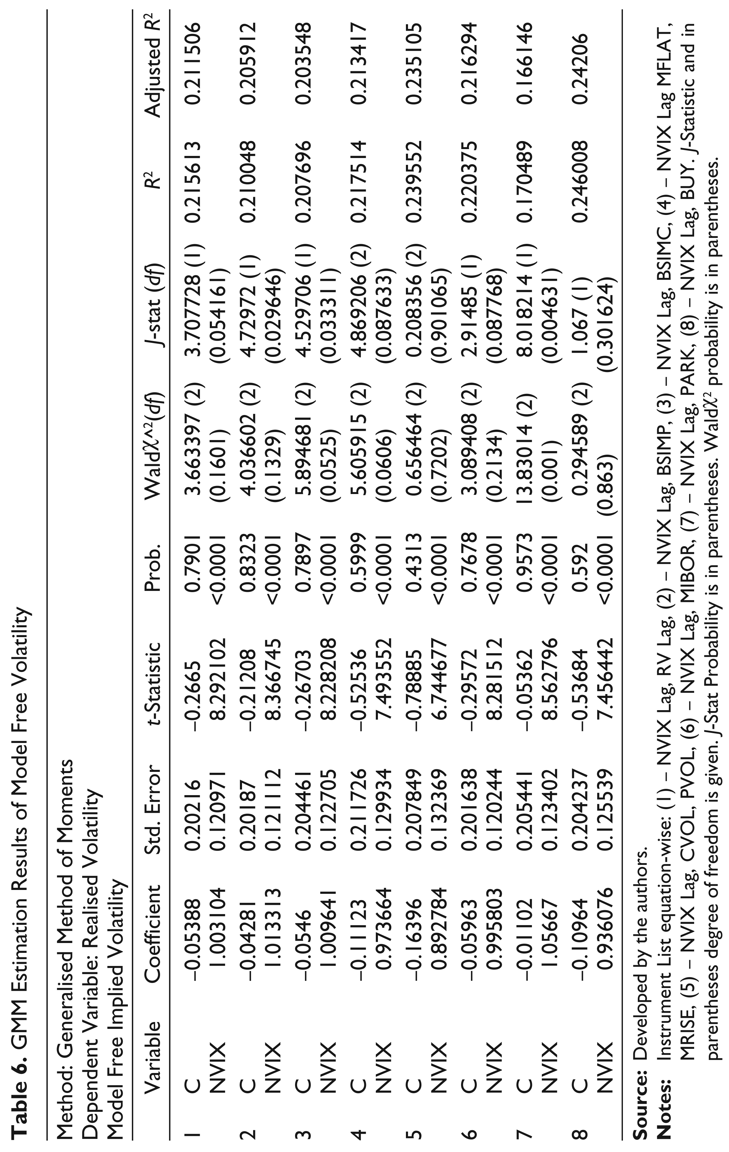
Notes: Instrument List equation-wise: (1) – NVIX Lag, RV Lag, (2) – NVIX Lag, BSIMP, (3) – NVIX Lag, BSIMC, (4) – NVIX Lag MFLAT, MRISE, (5) – NVIX Lag, CVOL, PVOL, (6) – NVIX Lag, MIBOR, (7) – NVIX Lag, PARK, (8) – NVIX Lag, BUY. J-Statistic and in parentheses degree of freedom is given. J-Stat Probability is in parentheses. Waldχ² probability is in parentheses.

Compared to Tables 4 and 5, the results clearly bring out that NVIX does not contain information about either call implied volatility or put implied volatility where as both of these volatilities subsume the information in NVIX. It is also not informative about the historical volatility. It does contain the information about the directional variables like MFLAT, MRISE and BUY. Also, it does contain information in volumes and short-term interest rates. Intuitively it supports the value of this index to represent the fear factor in the market, since it essentially indicates the direction of the market.

Historical Volatility

As per hypothesis in Equations (4) and (1), the Historical volatility is an unbiased estimate of the realised volatility. Also it contains all the information in the instrumental variables like MRISE, MFLAT which are directional variables, CVOL, PVOL, BUY, MIBOR, NVIX and PARK.

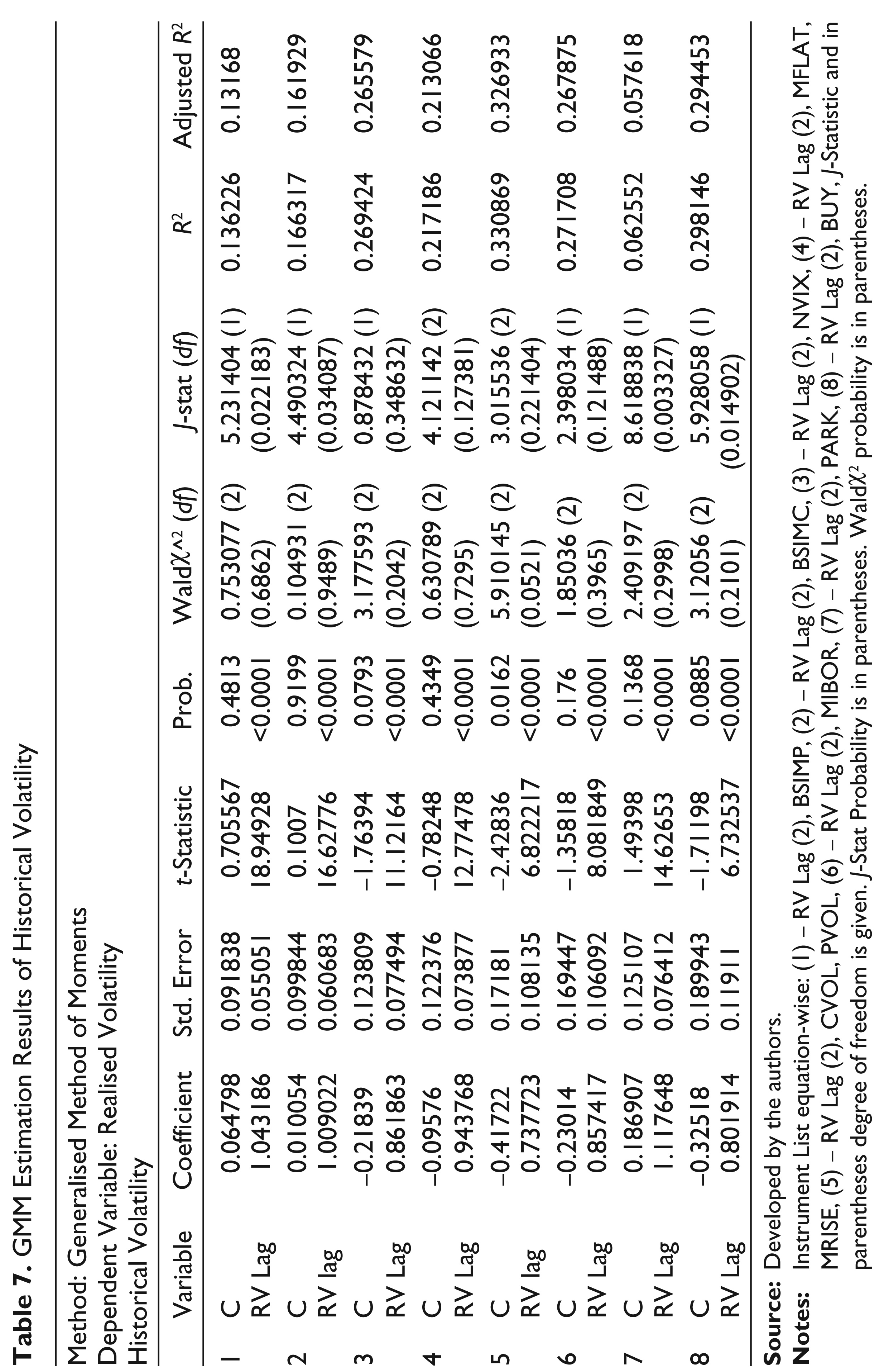
The results of the historical volatility as an estimate of future volatility are being presented in Table 7. The results from t-statistic suggest that in most of the regressions the intercept is not significant and the independent variable is highly significant. The Wald χ^2 statistic does not reject the hypothesis that α = 0 and β = 1 in all equations barring Equation (5). This suggests that the historical volatility is the unbiased estimate of the future volatility because of volatility persistence. Also, the explanatory power of historical volatility is least among others when compared to the previous regressions.

The J-statistic of Equations (1), (2), (7) and (8) suggest that it rejects the hypothesis that the over identifying restriction of the instruments like BSIMC, BSIMP, PARK, BUY are not significant. It can be said the historical volatility does not contain the information related to the model-based implied volatility measures. It also does not contain the information related to the range-based volatility and the directional variable. However, the J-statistic supports non rejection of the hypothesis for NVIX, MFLAT & MRISE, CVOL and PVOL and MIBOR. It is informative and subsumes information in model free volatility, directional variable, option volumes and interest rates. It is counter intuitive that historical volatility seems to contain information of direction as a trend but does not contain information of the direction of the market for the day. Also like all other volatility measures it contains information about option volumes and interest rates. There seems to be a very distinctive information in the model-based measures and model free measures. Historical volatility has no information about the model-based measures, while it has information about model-based measure perhaps that is because essentially NVIX indicates market direction and historical volatility also could indicate the direction provided volatility persists. However, the model-based measures could have additional information. Traders prefer trading in options market if they think that such trades are more beneficial. In that case the historical volatility and model-based volatility both evolve independently suggesting market inefficiency.

Table 7.

GMM Estimation Results of Historical Volatility

Method: Generalised Method of MomentsDependent Variable: Realised VolatilityHistorical Volatility
	Variable	Coefficient	Std. Error	t-Statistic	Prob.	Waldχ^² (df)	J-stat (df)	R²	Adjusted R²
1	C	0.064798	0.091838	0.705567	0.4813	0.753077 (2)	5.231404 (1)	0.136226	0.13168
	RV Lag	1.043186	0.055051	18.94928	<0.0001	(0.6862)	(0.022183)
2	C	0.010054	0.099844	0.1007	0.9199	0.104931 (2)	4.490324 (1)	0.166317	0.161929
	RV lag	1.009022	0.060683	16.62776	<0.0001	(0.9489)	(0.034087)
3	C	–0.21839	0.123809	–1.76394	0.0793	3.177593 (2)	0.878432 (1)	0.269424	0.265579
	RV Lag	0.861863	0.077494	11.12164	<0.0001	(0.2042)	(0.348632)
4	C	–0.09576	0.122376	–0.78248	0.4349	0.630789 (2)	4.121142 (2)	0.217186	0.213066
	RV Lag	0.943768	0.073877	12.77478	<0.0001	(0.7295)	(0.127381)
5	C	–0.41722	0.17181	–2.42836	0.0162	5.910145 (2)	3.015536 (2)	0.330869	0.326933
	RV lag	0.737723	0.108135	6.822217	<0.0001	(0.0521)	(0.221404)
6	C	–0.23014	0.169447	–1.35818	0.176	1.85036 (2)	2.398034 (1)	0.271708	0.267875
	RV Lag	0.857417	0.106092	8.081849	<0.0001	(0.3965)	(0.121488)
7	C	0.186907	0.125107	1.49398	0.1368	2.409197 (2)	8.618838 (1)	0.062552	0.057618
	RV Lag	1.117648	0.076412	14.62653	<0.0001	(0.2998)	(0.003327)
8	C	–0.32518	0.189943	–1.71198	0.0885	3.12056 (2)	5.928058 (1)	0.298146	0.294453
	RV Lag	0.801914	0.11911	6.732537	<0.0001	(0.2101)	(0.014902)

Source: Developed by the authors.

Notes: Instrument List equation-wise: (1) – RV Lag (2), BSIMP, (2) – RV Lag (2), BSIMC, (3) – RV Lag (2), NVIX, (4) – RV Lag (2), MFLAT, MRISE, (5) – RV Lag (2), CVOL, PVOL, (6) – RV Lag (2), MIBOR, (7) – RV Lag (2), PARK, (8) – RV Lag (2), BUY, J-Statistic and in parentheses degree of freedom is given. J-Stat Probability is in parentheses. Waldχ² probability is in parentheses.

All through our discussion above it is evident that the model-based measures have no information about historical volatility. Likewise, the historical volatility has no information about model-based volatility. This could mean that these markets have volatility-based arbitrage opportunities and such opportunities could be profitable.

Conclusions

The implied volatility measures, that is, both model-based Black Scholes and model free method (VIX) are biased and are partially inefficient. But they do have information content and there seems to be a mixed utility of both these methods. While Black Scholes implied volatility subsume information about short-term interest rates, option volumes and VIX itself the model free implied volatility does not subsume the information in model-based implied volatility. But it does seem to score a point in terms of information related to market direction. This could be due to the fact that more traders use Black Scholes for trading purposes than any other formula and therefore it seems to be more informative relative to the model free implied volatility. While one of the essential utility of model free implied volatility is to indicate whether the market is oversold (underpriced) or overpriced, VIX seem to indicate the direction of the market relative to the current underpricing or overpricing.

Also the results indicate that the Indian derivative markets offer volatility-based trading opportunities because both these markets could be functioning in a separating equilibrium, where trader may find trading information in option markets or in spot markets would be relatively more beneficial. Also, the model-based measures have higher explanatory power and they subsume information in model free measures which is a result contrary to Jiang and Tian (2005).

References

Amin

K.I.

V.K.

(1997), ‘Inferring Future Volatility from Information in Implied Volatility in Eurodollar Market: A New Approach’, Review of Financial Studies, 10: 333–67.

Andersen

T.G.

Bollerslev

(1998), ‘Answering the Critics, Yes ARCH Models Do Provide Good Forecasts’, Institutional Economic Review, 39: 885–905.

Andersen

T.G.

Bollerslev

Diebold

F.X.

Labys

(2001), ‘The Distribution of Exchange Rate Volatility’, Journal of the American Statistical Association, 96: 42–55.

Basu

Sankarshan

Mukhopadhyay

Bappaditya

(2006), ‘Derivatives in Asia Pacific Markets’, Journal of Emerging Markets Finance, 5(3): 207–15.

Becker

Clement

A.E.

White

(2006), ‘On the Informational Efficiency of S&P500 Implied Volatility’, The North American Journal of Economics and Finance, 17: 139–53.

Black

Scholes

(1973), ‘The Pricing of Options and Corporate Liability’, The Journal of Political Economy, 81(3): 637–54.

Britten-Jones

Neuberger

(2000), ‘Option Prices, Implied Price Processes and Stochastic Volatility’, Journal of Finance, 55: 839–66.

Canina

Figlewski

(1993), ‘The Information Content of Implied Volaitility’, Review of Financial Studies, 6: 659–81.

Chirstensen

B.J.

Prabhala

N.R.

(1998), ‘The Relation between Implied Volatility and Realized Volatility’, Journal of Financial Economics, 50: 125–50.

10.

Dacorogna

M.M.

Gencay

Muller

Olsen

R.B.

Pictet

O.V.

(2001), An Introduction to High Frequency Finance. California USA: Academic Press.

11.

Day

Lewis

(1992), ‘Stock Market Volatility and the Information Content of Stock Index Options’, Journal of Econometrics, 52: 267–87.

12.

Fleming

(1998), ‘The Quality of Market Volatility Forecast Implied by S&P 100 Index Option Prices’, Journal of Empirical Finance, 5: 317–45.

13.

Gupta

L.C.

(1996), Report of the Committee on Derivatives, Securities and Exchanges Board of India. Mumbai: SEBI.

14.

Harvey

C.R.

Whaley

R.E.

(1992), ‘Market Volatility Predictions and the Efficiency of S&P 100 Index Option Market’, Journal of Financial Economics, 31: 43–73.

15.

Harvey

Newbold

(2000), ‘Tests for Multiple Forecast Encompassing’, Journal of Applied Econometrics, 15: 471–82.

16.

Jiang

G.J.

Tian

Y.S.

(2005), ‘The Model Free Implied Volatility and Its Information Content’, Review of Financial Studies, 18: 1305–42.

17.

Jorion

(1995), ‘Predicting Volatility in the Foreign Exchange Market’, Journal of Finance, 50: 507–23.

18.

Lamoureux

C.G.

Lastrapes

(1993), ‘Forecasting Stock Return Variance towards Understanding Stochastic Implied Volatility’, Review of Financial Studies, 6: 293–326.

19.

Parkinson

(1980), ‘The Extreme Value Method for Estimating the Variance of the Return’, Journal of Business, 53: 61–65.

20.

Poon

S.H.

(2005), A Practical Guide to Forecasting Financial Market Volatility. England: John Wiley & Sons Ltd.

21.

Shanken

(1990), ‘Interporal Asset Pricing: An Empirical Analysis’, Journal of Economics, 45: 99–120.

22.

Sophie

Pan

Poteshman

A.M.

(2008), ‘Volatility Information Trading in the Option Market’, Journal of Finance, 58: 1059–91.

23.

Varma

J.R.

(1998), Risk Containment in the Derivatives Market, Securities and Exchanges Board of India.

24.

Vipul (2008), ‘Mispricing, Volume, Volatility and Open Interest: Evidence from Indian Futures Market’, Journal of Emerging Market Finance, 7(3): 263–92.